http://www.sciencepublishinggroup.com/j/ijiis doi: 10.11648/j.ijiis.20170603.11
ISSN: 2328-7675 (Print); ISSN: 2328-7683 (Online)
A Novel Approach of the Shortest Path Problem Using P
System
Einallah Salehi
Department of Computer Science, Malayer Branch, Islamic Azad University, Malayer, Iran
Email address:
To cite this article:
Einallah Salehi. A Novel Approach of the Shortest Path Problem Using P System. International Journal of Intelligent Information Systems. Vol. 6, No. 3, 2017, pp. 25-35. doi: 10.11648/j.ijiis.20170603.11
Received: June 9, 2017; Accepted: June 30, 2017; Published: July 20, 2017
Abstract:
Membrane Computing is inspired from biological cell activities as a new distributed parallel computational framework, which can be used for decreasing the time complexity of problems with high execution time. Since the usual way to reduce the time complexity of Artificial Intelligence (AI) problems is using parallel algorithms, Membrane Computing can be extensively applied. On the other hand, shortest path problem (SPP) is the most broadly method to solve the problems in AI. There have been a variety of algorithms presented, that could find a solution in a desirable time but usually are not accurate, or they are accurate but they are too slow. In Membrane Computing technique, the normal way for reducing the time complexity is using P system with active membranes that the number of membranes increases during the computation; thus, the time is traded against the space. This paper presents the first Membrane Computing technique for solving the SPP using P system with membranes division by a breadth first exploring on a grid. The theorems show the run times for breadth-first search and SPP are significantly reduced.Keywords:
Breadth-First Search, Division Rule, P System, Shortest Path Problem, Time Complexity1. Introduction
One of the areas of the study in computer science is Membrane Computing that has been proposed in [1]. Membrane Computing is a framework for the distributed parallel computing. This framework of computation has been derived from the views, the configurations, models and also living cell activities as well as the cells organized in a hierarchy. Through Membrane Computing, P system is gained and it is designed for this new parallel computing. In the initial configuration of a P system, there are several membranes that they are placed in the most outer membrane (skin). The membranes divide the Euclidean space into different and discrete regions that include several evolution rules and objects of alphabetical symbols. Through using these rules, it will become possible to change and/or transfer each object into the next region. Also the membranes could be dissolved, divided or created by some rules. The rules are usually applied in a maximally parallel and nondeterministic manner. The computation begins following the initial system configuration and it ends when it is not possible to apply any rule. The results of computation might be a multiset of
objects which accumulated in output membrane or is released from the skin of the system.
by them [6-10].
The shortest path problem (SPP) is used in order to find a path possessing hold the minimum travel cost, from one or more start point to one or more goal in a linked network. Since the range of applications in transportations, robotics, computer and networks, is broad, this case is a significant issue. In order to solve the SPP different methods were suggested. In approximate and heuristic algorithms, the solution was found in a sufficient time, while they may not be accurate in this period of time. Even if the accuracy is high, they might not be executed fast enough. One of the algorithms that have been already designed and proposed is finding the shortest path using breadth-first search (BFS) algorithm.
In this paper, a new parallel approach for finding the shortest path between two vertices (origin and destination) is introduced in which P system with division rules is used. This P system is explored a directed grid with m rows and n
columns of the nodes, which includes positive integer weights according to BFS. This method is capable to decrease the time complexity of BFS from O mn(3 ) to
[2( )]
O m+n , and also reduces the time complexity of SPP from O mn[ (2L+1)] to O[2 (L m+n)] assuming L as the maximum size length of the edges.
The paper is organized as follows: In section 3, some basic definitions on P system with division rules are presented. Section 4 introduces the SPP using the BFS algorithm. The proposed method for SPP using BFS algorithm based on P system with membrane division is presented in section 5, in which some guidelines on the implementation of a P system with membrane division for SPP are presented using the BFS algorithm. In section 6, using three examples, experiments carried out in this study are presented. Finally, in section 7, conclusion and some ideas for future works are described.
2. Related Works
The first approaches on searching problems in the framework of Membrane Computing have been already done by Gutiérrez-Naranjo and Pérez-Jiménez [11, 12]. In these studies depth-first search (DFS) and local search have been investigated using transition P systems and speed of execution time for solving the N-Queen problem have been extremely increased in comparison to prior work [13]. Moreover, P systems were utilized for studying on DFS and BFS in [14-16] on disjoint paths. In these researches, P systems are used without division rules. The first study has been presented by applying well-known Membrane Computing techniques for implementation of BFS using P system with membrane division. In this study the BFS algorithm has been imposed on a random binary tree that the time complexity will be decreased from exponential to linear with regard to the depth of the tree [17].
3. P System with Membrane Division
P system with membranes division is a model which has
been frequently studied on the Membrane Computing. This model is a well-known model in the P system community and one of the earliest models which emerged in 2001 [3].
Definition 1: A P system with division rules for elementary membranes (P system with active membrane using division rules for elementary membranes) is a construct of the form
1 2
( ,Γ IM,IN,OM,ON,H, ,µW R i, ,inp,ioutp )
Π = , where:
(1) Γ denotes the alphabet of symbol-objects. (2) IM ⊆Γ is the input alphabet.
(3) IN is the numerical input.
(4) OM ⊆Γ is the output alphabet. (5) ON is the numerical output.
(6) H indicates a finite set of labels for membranes. (7) µ stands for a membrane structure, consisting of finite membranes that labeled with elements of H.
(8) W ={mh h∈H}, where:
* h
m ∈Γ (Γ*is the set of strings overΓ ) describes the initial multiset of the objects placed in the membrane with label h.
(9) 1
{
}
1
, , , 0
p in
i p ∈ + − , denotes the input region (membrane).
(10) 2
{
}
2
, , , 0
p out
i p ∈ + − , determines the output region
(membrane).
(11) R stands for a finite set of rules of the following forms:
(a)
[
]
ph
x→u , for
{
}
*; , , 0 ; ,
h∈H p∈ + − x∈Γ u∈Γ .
This is an object evolution rule that is accompanied with a membrane which is labeled with h, and it depends on the membrane polarity. The empty string is represented by
* Γ
λ
∈ .(b)
[ ]
p1[ ]
p2h h
x → y , for h∈H p p, 1, 2∈ + −
{
, , 0 , ,}
x y∈Γ.An object is sent in from the immediate outside region of the membrane with the label h; at the same time, this object would be changed into another object, and, simultaneously, the membrane polarity can also be changed.
(c)
[ ]
p1[ ]
p2h h
x →y , for h∈H p p, 1, 2∈ + −
{
, , 0 , ,}
x y∈Γ.Here, an object is sent out from the membrane with the label h to the immediate outside region. This object, at the same time, changes into another object, and, simultaneously, the membrane polarity can be changed.
(d)
[ ]
xhp →y, for h∈H; p∈ + −{
, , 0 ; ,}
x y∈Γ.A membrane labeled with h is dissolved in reaction with an object. The skin is never dissolved.
(e)
[ ]
p1[ ] [ ]
p2 p3h h h
x → y z , for
{
}
1 2 3
; , , , , 0 ; , ,
h∈H p p p ∈ + − x y z∈Γ.
A membrane by an object can be divided into two membranes with the same label, each of them containing one object (objects may be the same or different). And the polarities of these membranes can be altered.
The rules of a P system with membrane division are employed based on the following principles:
step, one object of a membrane could be utilized by only one rule that is chosen in a non deterministic way, but any object that is able to evolve by one rule of any form should do its evolution.
(2) With dissolution of a membrane, its contents (multiset and internal membranes) are left free in the surrounding region.
(3) All objects and membranes that have not been specified in a rule and those that have not evolved remain unchanged to the next step.
(4) Those rules that are associated with the membranes that are labeled with h are utilized for the all copies of this membrane. At one step, a membrane that is labeled with h
could only be subjected to one rule of types (b)-(e), and rule (a) could also be applied with other rules. In this case, assumption is that the evolution rules of type (a) are used first, and after that, the other types of rules are applied. This process takes only one step to be performed.
(5) The skin membrane could not be divided. Like other membranes, it can have “electrical charge”.
Note 1: In the above definition, some properties can be intended as follows;
(a). The non-necessary components of a P system can be omitted.
(b). Several inputs and outputs can be considered. (c). The numerical inputs and outputs can be considered
as a set of non-negative integer numbers, or vectors with non-negative integer components.
Definition 2: One says that rule ri has priority (in the
strong sense) over rule rj; if ri can be applied, then rule rj
cannot be applied. In this case one shows ri>rj.
Definition 3: Let ioutp be an output membrane (region) of P
system Π; one says that p2 out
i is a dynamic output if the P system rules can apply on p2
out
i .
This definition allows finding the different solution (using division rule, more than one solution can be obtained) of the problem. Also the number of steps will decrease (there is no need to transfer the output alphabets).
Definition 4: The number of objects in string u is the
length of the string, and it is denoted by u, also the number of objectain stringuis denoted by ua.
Remark 1: Some remarks are taken as follows:
(a). P system Π configuration in step i is determined by ( )
i
C Π (in short Ci); also, C0( )Π and CTΠ( )Π are
initial and final (halting) configurations, respectively. (b). The execution time (steps) of P system Π from
( )
i
C Π until final configuration is indicated by
( i( ))
T C Π , and therefore, 0
( ( ))
T C Π =TΠ.
(c). P system Πwith set of rules R is denoted by
R
Π .
Note 2: According to Remark 1(c):
0
( ( )) ( k( )), 0
T C Π = +k T C Π ≤ ≤k TΠ.
It should be noted that in a P system with membranes division, the number of membranes can be increased applying rules of type (e). Due to maximal parallelism, 2n copies from the membranes of the same labels can be obtained after n steps. Therefore, hard problems such as NP-complete problems or problems with high time complexity can be solved in this framework in a polynomial or even linear time.
4. The Shortest Path Problem Based on
Breadth-First Search Algorithm
The SPP deals to find the shortest distance between start and final vertices in a graph in which shown by a set of edges and nodes. The SPP is a most basic network optimization problem that in a plenty of network optimization algorithms, this problem may happen and be considered as sub problem. Different types of SPP algorithms are being introduced and improved constantly.
There are several algorithms to solve the SPP. One of the basic methods is the BFS algorithm, in which each level of the nodes will be expanded in one stage. Thus, if a node is placed in depth n, then it will be explored after n stages [18]. Hence, using breadth first can obtain the goal in the minimum number of stages. The approximate running time of BFS is O V( + E), where V is the number of vertices and E is the number of edges, also the time complexity for SPP using BFS is O V( +L E), in which L indicates the highest magnitude length of the edges [18, 19].
5. Proposed Method
This section provides the mentioned approach to solving the SPP based on BFS through P system with membranes division. This approach intends to prove that Membrane Computing can offer components required for finding a solution for any problem which as shown as a space of states; thus, it has a high capability to solve a wide range of the real-life problems. The aim of this approach is looking for a shortest path solution in the search space (weighted, directed grid) by using a class of P systems with membranes division according to the BFS.
5.1. Shortest Path Problem Formulation and Its Ingredients
In the present research, the SPP was executed based on BFS while P systems with membranes division were employed on a 2-dimentional directed grid with integer positive weights. Grids are an important restricted class of graphs which can reach a wide range of real-life problems using them.
connected to vertex vi+1,j (1≤ ≤ −i m 1, and 1≤ ≤j n ), or
vertex vi+1,j (1≤ ≤i m, and 1≤ ≤ −j n 1), or both of them.
A 2-dimentional directed grid graph is presented as G→m n×
and weighted graph G→m n× is considered as case study. The goal is finding the shortest path from origin ( v1,1) to
destination ( vm n, ). In this case, length of each edge is considered weight of it. Also length of each path from origin to destination is the summation of whole weights of the edges in each path, and the shortest path is a path with minimum length among the existing paths from origin to destination.
Remark 2: Some remarks of the case study (weighted
graph Gm n
→
× ) are considered as follows:
(a). Graph G→m n× is weighted by a positive integer numbers.
(b). Weight of edge (vi−1,j,vi j, ) is shown by wi j, ,1, where
2≤ ≤i m, and 1≤ ≤j n.
(c). Weight of edge(vi j,−1,vi j, )is shown bywi j, ,2, where
1≤ ≤i m, and 2≤ ≤j n.
(d). The connection between nodes vi−1,j and vi j,
(2≤ ≤i m, and 1≤ ≤j n) is considered by
, ,1 , ,1
1 , if there exist the connection ,
0 , if there exist no the connecttion
i j i j
y y =
.
(e). The connection between nodes vi j, −1 and vi j,
(1≤ ≤i m, and 2≤ ≤j n) is considered by
, ,2 , ,2
1 , if there exists the connection ,
0 , if there exists no the connection
i j i j
y y =
.
(f). The origin (start state) and destination (final state) vertices areO=v1,1andD=vm n, , respectively.
Note 3: Each path from O to D is in the form
1 1, 2,2 , 1, 1 ,
( , ) ( i j, i j ,..., ik jk, ik jk ,..., i jl l )
P O D = O=v v v v + + v =D , such
that the connection between vertices vik,jk and vik+1,jk+1 is
according to Definition 5. Without prejudice to the generality of the definition, P O D( , ) can be considered such as
1 1, 2,2... k,k k 1,k 1... l,l
i j i j i j i j i j
v v v v + + v .
5.2. General View of the Proposed Method
This subsection is given an overview design of a P system family with membrane division for solving the SPP according to BFS on the case study. The computation has two phases; phase one is to find the paths from O to D
according to BFS, and phase two is finding the shortest path among the discovered paths. The gist of the research is as follows:
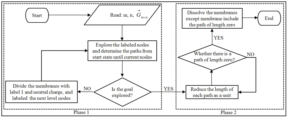
Figure 1. Logical scheme.
Phase 1: At each stage of the computation, the system (P system) explores the labeled nodes (in initial configuration the origin is explored), next, it checks to find the goal (destination). If the goal is explored then the computation will be entered to phase two, and if the goal is not explored then the membranes with label 1 (elementary membrane that located in the skin) will be divided and the next level nodes are labeled and the process will be continued until the goal is found. Considering the fact that each level of graph is
explored in one stage, and if the goal exists at the depth d, the goal will be discovered after d+1 stages. In section 5.3, it will be demonstrated that each stage takes 2 steps. After finding the goal, phase two will begin.
computation will be halted. In this case the remaining multisets in membrane labeled 1 show the shortest path from
O to D (see the proposed method in Figure 1).
5.3. P System Algorithm for Solving the Shortest Path Problem
As all know algorithms that are compatible with common architectures are executed sequentially, thus, many problems in artificial intelligence are implementable using these architectures consecutively with high time complexity. P system is a new parallel framework which allows solving the hard problems in a feasible time.
Here is a solution to solve the SPP using P system with membranes division that the aim is to solve the SPP
according to BFS on Gm n
→
× . In this framework the time
complexities for BFS and SPP are O[2(m+n)] and [2 ( )]
O L m+n , respectively, in which L is the maximum size length of the edges; whiles these complexities in sequential algorithm are O V
(
+ E)
=O(
3mn)
and(
)
[ (2 1)]O V +L E =O mn L+ , respectively. The details for obtaining this idea and P system structure are given bellow.
Proposed P system: P system
( , , , , , , , , p )
N M N out
Π= Γ I O O H µW R i is considered with
dynamic output and with the strong priorities r1>r2 and
7 8
r >r where:
(a) Numerical input IN =
{ } {
m n, ∪ 0,1, 2, 3,...,L}
, where,
m n∈N.
(b) Working alphabet
{
, , , ,}
{
i j, , i j, 1 , 1}
Γ = d g p s w ∪ a v ≤ ≤i m ≤ ≤j n
{
ci j, ,1 2≤ ≤i m , 1≤ ≤j n} {
ci j, ,1i = +m 1, 1≤ ≤ −j n 1}
∪ ∪
{
ci j, ,21≤ ≤i m , 2≤ ≤j n} {
ci j, ,2 j = +n 1, 1≤ ≤ −i m 1}
∪ ∪
(c) Output membrane ioutp 1
+
= .
(d) Output alphabet OM =
{
vi j, 1≤ ≤i m , 1≤ ≤j n}
.(e) Numerical output ON =
{ }
uw , where, u is themightiest in the output region. (f) The set of labels H ={0,1}.
(g) Initial membrane structure 0 0 1 0
[ [ ] ]
µ= .
(h) The set of initial multisets W={m m0, 1} , where,
0
m =g,m1=a v1,1 1,1.
The set of rules R are also considered as follows:
0
1 [ m n, ]1 m n, []1
r ≡ a →a −
After applying this rule, the object am n, will be sent
outside, and the polarity of membrane 1 is changed from neutral to negative. This rule will be applied when there is the final state in membrane 1, and after that phase two will be started.
0 0 0
2 [ i j, ]1 [ i 1, ,1 1j ] [ i j, 1,2 1] ; 1 , 1
r ≡ a → c+ c + ≤ ≤i m ≤ ≤j n
Object ai j, divides the membrane 1 and sends ci+1, ,1j and
, 1,2 i j
c + to the core of each new membrane, that they labeled next level nodes, and they will explore the next level nodes in the next step (see r5).
0
3 [ m 1, ,j k]1 ; 1 , 1 2
r ≡ c + →d ≤ ≤j n ≤ ≤k
0
4 [ i n, 1,k]1 ; 1 , 1 2
r ≡ c + →d ≤ ≤i m ≤ ≤k
By applying rules of type r3 and r4, the membranes that
they observe outside of the graph structure will be dissolved.
( , ,)
{
}
{ }
, , , , , , 1 0
5 [ , , , , ] ; 11 , 1 , 1 2, , , 0,1, 2,..., , , , 0,1
i j k
i j k i j k i j k y
w w y
i j k i j i j i j k i j k
r ≡ c →w p v a s − ≤ ≤i m ≤ ≤j n ≤ ≤k w ∈ L y ∈
From ci j k, , , rule r5 makes , , i j k
w
w (weight of the edge),
, , i j k
w
p (for finding the shortest path by rule r7 ), vi j,
(explored node), and one copy of ai j, or
s
(not both). If, , 1 i j k
y = , then there is one copy ai j, that labels the next level
nodes in the next step by rules r2 and the process will
continue. If yi j k, , =0 , then there exist not connection
between current and next level nodes, in this case one copy of object
s
will be appeared and the computation will be stopped in this path in the next step by rule r6.0 6
[ ]
1r
≡
s
→
d
This rule is applied when there exists no connection between current and next level nodes (see r5). Using this
rule, the membrane with label 1 is dissolved, and computation will be stopped in this path.
7 [ ]1 []1
r ≡ p−→p −
By this rule, a copy of p is sent out from the membrane with the label 1 and negative charge in each step. Beginning of working this rule is start of phase two.
8 []1 [ ]1
r ≡g −→ g+
Objectgis sent into membrane 1, and, simultaneously, the membrane polarity is changed from negative to positive. This membrane contains the shortest path from origin to destination.
Note 4: In this paper, for the notational convenience, multiset
1 1, 2,2... t,t t1,t 1... l,l
i j i j i j i j i j
where 1≤ ≤it m , 1≤ ≤jt n , and it+1=i jt, t+1= +jt 1 , or
1 1, 1
t t t t
i+ = +i j+ = j . Also, the summation
1 1, ,1 2,2,2 ... t, ,t t t1,t 1,t1 ... l, ,l l
i j k i j k i j k i j k i j k
w +w + +w +w+ + + + +w and the sequence yi j k1 1, ,1,yi2,j k2,2,...,yi j kt, ,t t,yit+1,jt+1,kt+1,...,yi j kl, ,l l are
shown by δi jl,l and λi jl,l , respectively, where
1,1
1≤ ≤it m , 1≤ ≤jt n,δ =0, and it+1=i jt, t+1= +jt 1,kt=2,
or it+1= +it 1,jt+1= j kt, t=1 . Note that in all of above
relations m n, ∈N.
Lemma 1: Let Π be the proposed P system with mentioned components such that yi j k, , =1, for all yi j k, , , and
let Ai j, and δi j, be parameters according to Note 4. If C is an
arbitrary computation of the system and 2≤ ≤ +K m n, then the multiset associated with membrane 0
1 (membrane with label 1 and neutral charge) is in the form , ,
, ,
i j i j
i j i j
wδ pδ A a in the configuration C2(K−2), and in this case i+ =j K.
Proof: See Appendix A.
Lemma 2: Let C be an arbitrary computation of the
proposed P system. Consider the parameters Ai j, ,δi j, , and
, i j
λ according to Note 4, and let the terms of sequence λi j, and the objects of multiset Ai j, have matched indexes. For
each K (2≤ ≤ +K m n) the following holds:
(a). If each term of the sequence λi j, is equal 1, then for
configuration 2(K 2)
C − , there exists a unique membrane1 whose associated multiset is in the form0
, ,
, ,
i j i j
i j i j
wδ pδ A a , such that i+ =j K.
(b). If yi j k, , =0 (i+ =j K) is the first term of sequence
, i j
λ that it is equal 0, then the membrane 1 0
containing multiset Ai j, will be dissolved in
configuration C2(K− +2) 1.
Proof: See Appendix B.
Lemma 3: Let R′ be a set of rules such as
1 2 3 4 5 6
{ , , , , , }
R′ = r r r r r r , and let Ai j, , δi j, and λi j, be
according Note 4. If Π is the proposed P system with mentioned ingredients, then:
0
( ΠR)) 2( 2) 1
T C ( ′ ≤ m+ − +n .
Also, if exists a sequence λi j, with terms of equal 1, then:
0
( Π )) 2( 2) 1
R
T C ( ′ = m+ − +n
Proof: See Appendix C.
Theorem 1: If Gm n
→
× is the case study, then the BFS
algorithm runs in [2(O m+n)] on Gm n
→
× by a P system with
division rules.
Proof: See Appendix D.
Lemma 4: Let Ai j, ,δi j, and λi j, be according to Note 4,
and let exists a sequence λi j, that its terms are equal 1. If C
is an arbitrary computation of the proposed P system with the mentioned ingredients, then the following holds:
(c). A membrane 1+ containing multiset ,
,
m n
m n
gwδ A will
be obtained, in configuration 1 ,
2(m n 2) Min{m n} 2
C
δ −
+ − + +
, where , ,
1
{ }
m n Min m n
δ = − δ .
(d). 2( 2) 1 1 , 1 , 1 ,
, , ,
1 1 1
{ } , { } { }
( ( ))
{ } 1 , { } { }
m n m n m n
m n
m n m n m n
Max Max Min
T C
Min Max Min
δ δ δ
δ δ δ
− − −
− − −
+ − + Π = >
+ =
.
Proof: See Appendix E.
Lemma 5: Letδi j, andλi j, be according to Note 4, and let
exists a sequence λi j, that its terms are equal to 1. IfΠis the
proposed P system with the mentioned ingredients, then:
, , ,
1 1 1
0
, , ,
1 1 1
2( 2) { } 1, { } { }
( ( ))
2( 2) { } 2, { } { }
m n m n m n
m n m n m n
m n Max Max Min
T C
m n Min Max Min
δ δ δ
δ δ δ
− − −
− − −
+ − + + >
Π =
+ − + + =
Proof: See Appendix F.
Theorem 2: If Gm n
→
× is the case study, then the SPP
algorithm runs in [2(O m+n)] on Gm n
→
× by a P system with
division rules, in which L is the maximum magnitude length of the edges.
Proof: See Appendix G.
6. Simulations
In this section, the ability of this technique is shown by following the computation of the examples that were shown in Figures 2 and 5.
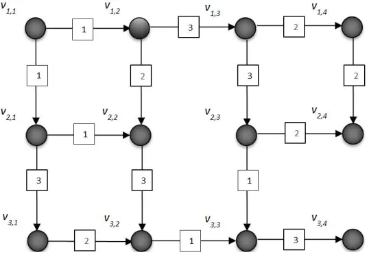
Example 1:The goal is to find the shortest path from v1,1
to v3,4 in the weighted graph G3 4
→
× , which it is shown in
Figure 2 by proposed P system. In this case, m=3,n=4,
, 1
{ m n} 8
Minδ
− = , and , 1
{ m n} 11
Maxδ
− = . By Lemma 3, whole of
paths will be obtained in configuration 2(m n 2) 1 11 C + − + =C , and from Lemma 5, the shortest path will be achieved in
configuration 1 ,
2( 2) { } 1 22
m n
m n Max
C C
δ −
+ − + +
= . The paths from v1,1
(start) to v3,4 (goal) are available in the membranes 1
− and
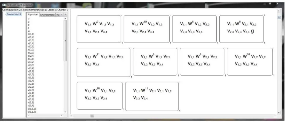
1+, which the shortest path is accessible in membrane 1+. Numerical output (power of ) shows the weight of path and output objects show the path. For verification, the program has run in the P-Lingua [20]. The final configuration (Configuration 22) is shown by P-Lingua simulator in Figure 3.
Figure 2. Weighted graph G→3 4× , with positive integer weights mentioned in Example 1.
Figure 3. The final configuration of the proposed method for finding the shortest path in weighted graph G3 4 →
× mentioned in Figure 2 by P-Lingua simulator.
Example 2: The goal is to find two paths with a minimum length among the whole of paths in Example 1. It is enough to consider m0=g2 as the initial multiset in region 0. In this case, there will be two membranes 1
+
in the final configuration that they show two paths. The simulation is carried out using P-Lingua shown in Figure 4.
Example 3: The goal is to find the shortest path from v1,1 to v3,4 in non-complete weighted graph G3 4
→
× , which it is shown in
Figure 5 by the proposed P system. The whole process is according to Example 1, but with fewer paths. The final configuration of the example simulation using P-Lingua is visible in Figure 6.
Figure 5. Non-complete weighted graph G→3 4× , with positive integer weights mentioned in Example 3.
Figure 6. The final configuration of the proposed method for finding the shortest path in non-complete weighted graph
3 4
G→ × mentioned in Figure 5 by P-Lingua simulator.
7. Conclusion and Future Works
In this study, a novel parallel approach based on P system has been presented to find the shortest path between two points according to the breadth-first search (BFS) in a grid with m rows and n columns of the nodes. The proposed P system works based on membranes division, and it increases the workspace during the computation and decreases the time complexity. This method reduces the time execution of BFS from O mn(3 ) to O[2(m+n)] and the running time of SPP from [O mn(2L+1)] to [2 (O L m+n)] on the mentioned grid, where L is as the maximum length of the edges. As the future works, improvement of the proposed P system is suggested, considering the design and its ingredients. Also, investigation
of the problem on a new case study such as arbitrary graphs, and implementation of the study on the graphics processing unit (GPU) is recommended.
Appendix A - Proof of Lemma 1
The lemma is proved by induction on K.
Case 1 (K=2): In initial configuration (C0), there exist only one membrane 1 , such that its associated multiset is 0
1,1 1,1
1,1 1,1 1,1 1,1
v a =wδ pδ A a , thus the proposition is true for
2
K= .
in the form , ,
, ,
i j i j
i j i j
wδ pδ A a in configuration 2(K 2)
C − , and in this case i+ =j K. In the next step rules r2 can be applied
and membranes 0
1 will be duplicated; half of them including
, ,
, 1, ,1
i j i j
i j i j
wδ pδ A c+ , and the remaining including
, ,
, , 1,2
i j i j
i j i j
wδ pδ A c + , in this time, configuration C2(K− +2) 1 will be obtained. In the step 2(K− + =2) 2 2((K+ −1) 2), objects
1, ,1 i j
c+ and ci j,+1,2 are changed to 1, ,1 1, ,1
1, 1,
i j i j
w w
i j i j
w + p + v+ a+ , and
, 1,2 , 1,2
, 1 , 1
i j i j
w w
i j i j
w + p + v +a + , respectively, by rulesr5. Therefore,
in configuration C2((K+ −1) 2), each membrane 1 contains a 0
multiset such as follows:
, 1, ,1 , 1, ,1 1, 1,
, ,
, 1, 1, 1, 1,
, , , 1 ,
δ δ δ δ
δ δ
+ + + +
+ +
+ + = + +
= = + =
i j i j i j i j i j i j
I J I J
w w
i j i j i j i j i j
I J I J
w p A v a w p A a
w p A a I i J j
(1)
, , 1,2 , , 1,2 , 1 , 1
, ,
, , 1 , 1 , 1 , 1
, , , , 1
δ δ δ δ
δ δ
+ + + +
+ +
+ + = + + =
= = +
i j i j i j i j i j i j
I J I J
w w
i j i j i j i j i j I J I J
w p A v a w p A a
w p A a I i J j
(2)
in this case I+ = +J K 1.
Now, let i=m j, <n or i<m , j=n therefore, some membranes 0
1 include am j, or ai n, , in configuration 2(K 2)
C − .
For these membranes, configuration C2(K− +2) 1 are obtained by applying rules r2, and these membranes will be divided;
each of them containing an object cm+1, ,1j or ci n,+1,2, that in
the next configuration (C2((K+ −1) 2)) will be dissolved by rules
3
r and r4, and thus the lemma holds for K.
Appendix B - Proof of Lemma 2
(a) If yi j k tt, ,t =1 , for each
, , , (1 ,1 ,1 2)
t t
i j k t i j t t t
y ∈λ ≤ ≤i i ≤ ≤j j ≤ ≤k , then by considering the proof of Lemma 1 it is deducted that there exists a unique membrane 0
1 whose associated multiset is in the form , ,
, ,
i j i j
i j i j
wδ pδ A a , such that i+ =j K.
(b) By hypothesis, if yi j k tt, ,t ∈λi j, , then yi j k tt, ,t =1 and
, , 0 i j k
y = , where 1≤ < =it il i , 1≤ < =jt jl j , 1≤ ≤kt 2 .
Tues, by part (a), there exists a unique membrane1 whose 0 associated multiset is in the form
, ,
1 1 1 1
1, 1 1, 1 il jl l jl
l l
i
i j i j
wδ− − pδ− − A a
− − − − in configuration
2((K 1) 2)
C − − ,
such that il+ = −jl K 1. In this configuration rules r2 and
after that rules r5 can be applied. In this case, membrane 1 0
with multiset associated , ,
,
i j i j
i j
wδ pδ A s will be obtained, in configuration C2(K−2). Now, for this membrane rule r6 can be applied and membrane will be dissolved, in configuration
2(K 2) 1
C − + . Therefore, membrane 1 containing multiset 0 Ai j,
will be dissolved in configuration C2(K− +2) 1.
Appendix C - Proof of Lemma 3
From Lemmas 1 and 2, and their proofs, if exist some membranes 1 in configuration 0 2( 2)
( )
m n
C + − Π , then each of these membranes contain a multiset in the form
, ,
, ,
m n m n
m n m n
wδ pδ A a or , ,
,
m n m n
m n
wδ pδ A s . The next configuration is obtained by applying rules r1 and r6
simultaneously. In this case the membranes containing multiset , ,
,
m n m n
m n
wδ pδ A s will be dissolved by applying rule
6
r ; and objet am n, will be sent out of membranes 0
1
containing multiset , ,
, ,
m n m n
m n m n
wδ pδ A a by applying ruler1, and the charge of membrane 0
1 is changed to negative, simultaneously, and configuration 2( 2) 1
( )
m n
C + − + Π is obtained. Thus, considering R′ ={ , , , , , }r r r r r r1 2 3 4 5 6 computation will be halted for P system ΠR′, in configuration 2( 2) 1
(Π )
m n
R
C + − + ′ .
Appendix D - Proof of Theorem 1
Let Gm n
→
× and its ingredients be according to Definition 5
and Remark 2, and let Π
R′ be mentioned P system in
Lemma 3 with output membrane 1− . If
1 1 2 2 1 1
1,1 , 1,1 , , , , , ,
( , m n) ( i j, i j ,..., ik jk, ik jk ,..., i jl l m n)
P v v = v =v v v v + + v =v
is a path from origin to destination, then according to Remarks 2(iv) and 2(v), the terms of sequence
1 1, ,1, 2,2,2,..., t, ,t t, t 1,t1,t1,..., l, ,l l
i j k i j k i j k i j k i j k
y y y y+ + + y are equal to 1. From Lemma 3 and its proof using P system Π
R′ with
numerical input according to the ingredients of Gm n
→
× , exists
a membrane 1− containing multiset , ,
,
m n m n
m n
wδ pδ A in configuration C2(m n+ − +2) 1. Considering Am n, ≡P v( 1,1,vm n, ), it
is deduced that, P system Π
R′ explores path P v( 1,1,vm n, ) in
[2( )]
O m+n . Also by Lemma 2, each path from v1,1 until
, i j
v will be explored in 2(K−2) steps, where K= +i j, it means the searching is based on BFS.
Appendix E - Proof of Lemma 4
(a) From proofs of Lemmas 1 and 2, the membrane structure of P system Π includes a skin and some membranes 0
1 , whose associated multisets are in the form
, ,
, ,
m n m n
m n m n
wδ pδ A a , in configuration 2(m n 2)
C + − , and by proof
of Lemma 3, the membranes will be changed to 1− including multiset in the form , ,
,
m n m n
m n
wδ pδ A , in configuration
2(m n 2) 1
with priority r7>r8 ; thus, rule r7 will be applied for
, 1
{ m n}
Minδ
− times, and one copy of object will be sent out
from each membrane 1− in each step. In this time, configuration 1 ,
2(m n 2) Min{m n} 1
C
δ −
+ − + +
is obtained, and some membranes 1− are empty from object p, these membranes are considered with label (1 )− ′. Next, rules r7 and r8 will be applied for membranes 1− and (1 )− ′, simultaneously. By applying rule r7, an object p will be sent out of membrane 1−, and by applying rule r8, object will be sent in of one of the membranes (1 )− ′, and changes the polarity of membrane
(1 )− ′ from negative to positive, and configuration
, 1
2(m n 2) Min{m n} 2
C
δ −
+ − + +
will be obtained with a membrane 1+, containing multiset ,
,
m n
m n
gwδ A , where , ,
1
{ }
m n Min m n
δ = − δ .
(b) From part (a), if { , } { , } 1
1
Max Min
m n m n
δ > δ
−
− , then
rule r7can be applied on some of the membranes 1−, from
configuration 2(m n 2) 1
C + − + until configuration ,
1
2(m n 2) Max{m n} 1
C
δ −
+ − + + , and computation will be halted. Also, if
{ } { }
, ,
1 1
Max Min
m n m n
δ = δ
−
− , then according to part (a), computation is halted in configuration ,
1
2(m n 2) Min{m n} 2
C
δ −
+ − + + .
Appendix F - Proof of Lemma 5
By Lemma 4(a), 0
( ( )) 2( 2) 1
T C Π > m+ − +n ; thus,
considering Note 2:
0 2( 2) 1
( ( )) [2( 2) 1] ( m n ( ))
T C Π = m n+ − + +T C + − + Π
then, the proof follows from Lemma 4(b).
Appendix G - Proof of Theorem 2
Let Gm n
→
× and its ingredients be according to Definition 5
and Remark 2. On one hand, from the proof of Theorem 1, whole of paths from origin to destination are explored in
m n G
→
× based on BFS using proposed P system Π in
configuration C2(m n+ − +2) 1. On the other hand, each δm n, is the length of a path from origin to destination, and after finding the shortest path as mentioned in Lemma 4(a), the computation will be halted. Also, by Lemma 5,
, , ,
1 1 1
0
, , ,
1 1 1
2( 2) { } 1, { } { }
( ( ))
2( 2) { } 2, { } { }
m n m n m n
m n m n m n
m n Max Max Min
T C
m n Min Max Min
δ δ δ
δ δ δ
− − −
− − −
+ − + + >
Π =
+ − + + =
and in the worst case δ =m n, (m n+ −2)L, where L is the
maximum magnitude length of edges; then,
0
( ( )) 2( 2) 2
T C Π = m n+ − L+ ,
which concludes the proof.
References
[1] Păun, G., Computing with Membranes. Journal of Computer and System Sciences, 2000. 61(1): p. 108-143.
[2] Păun, G., Membrane computing: an introduction. 2012: Springer Science & Business Media.
[3] Păun, G., P systems with active membranes: attacking NP complete problems. Journal of Automata, Languages and Combinatorics, 2001. 6(1): p. 75-90.
[4] Krishna, S. N. and R. Rama, A variant of P systems with active membranes: Solving NP-complete problems. Romanian Journal of Information Science and Technology, 1999. 2(4): p. 357-367.
[5] Mutyam, M. and K. Krithivasan, P Systems with Membrane Creation: Universality and Efficiency, in Machines, Computations, and Universality, M. Margenstern and Y. Rogozhin, Editors. 2001, Springer Berlin Heidelberg. p. 276-287.
[6] Frisco, P., M. Gheorghe, and M. J. Pérez-Jiménez, Applications of Membrane Computing in Systems and Synthetic Biology. 2014: Springer.
[7] Peng, H., et al., An automatic clustering algorithm inspired by membrane computing. Pattern Recognition Letters, 2015. 68: p. 34-40.
[8] Chen, H., et al., On trace languages generated by (small) spiking neural P systems. Theoretical Computer Science, 2016.
[9] Wang, J., P. Shi, and H. Peng, Membrane computing model for IIR filter design. Information Sciences, 2016. 329: p. 164-176.
[10] Song, B., T. Song, and L. Pan, A time-free uniform solution to subset sum problem by tissue P systems with cell division. Mathematical Structures in Computer Science, 2017. 27(1): p. 17-32.
[11] Gutiérrez-Naranjo, M. and M. Pérez-Jiménez, Depth-First Search with P Systems, in Membrane Computing, M. Gheorghe, et al., Editors. 2011, Springer Berlin Heidelberg. p. 257-264.
[12] Gutiérrez-Naranjo, M. A. and M. J. Pérez-Jiménez, Implementing local search with Membrane Computing. 2011. [13] Gutiérrez-Naranjo, et al. Solving the N-Queens puzzle with P
systems. in 7th Brainstorming Week on Membrane Computing. 2009. Sevilla, España: Fénix Editora.
p
[14] Michael J. Dinneen, Y. -B. K., and Radu Nicolescu, Edge- and node-disjoint paths in P systems, in Electronic Proceedings in Theoretical Computer Science 2010. p. 121-141.
[15] Nicolescu, R. and H. Wu, BFS Solution for Disjoint Paths in P Systems, in Unconventional Computation, C. Calude, et al., Editors. 2011, Springer Berlin Heidelberg. p. 164-176. [16] Nicolescu, R. and H. Wu, New solutions for disjoint paths in P
systems. Natural Computing, 2012. 11(4): p. 637-651. [17] Salehi, E., S. M. Shamsuddin, and K. Nemati, A Linear Time
Complexity of Breadth-First Search Using P System with
Membrane Division. Mathematical Problems in Engineering, 2013. 2013: p. 11.
[18] Russell, S. J. and P. Norvig, Artificial Intelligence: A Modern Approach(2nd Edition) 2ed. 2002: Prentice Hall.
[19] Even, S. and E. Guy, Graph algorithms. 2nd ed. 2012, Cambridge, NY: Cambridge University Press. xii, 189 p. [20] Díaz-Pernil, D., et al., A P-Lingua Programming Environment