Fast String Kernels using Inexact Matching for Protein Sequences
Christina Leslie [email protected]
Center for Computational Learning Systems Columbia University
New York, NY 10115, USA
Rui Kuang [email protected]
Department of Computer Science Columbia University
New York, NY 10027, USA
Editor: Kristin Bennett
Abstract
We describe several families of k-mer based string kernels related to the recently presented mis-match kernel and designed for use with support vector machines (SVMs) for classification of pro-tein sequence data. These new kernels – restricted gappy kernels, substitution kernels, and wildcard kernels – are based on feature spaces indexed by k-length subsequences (“k-mers”) from the string
alphabetΣ. However, for all kernels we define here, the kernel value K(x,y)can be computed in
O(cK(|x|+|y|))time, where the constant cK depends on the parameters of the kernel but is
inde-pendent of the size|Σ|of the alphabet. Thus the computation of these kernels is linear in the length
of the sequences, like the mismatch kernel, but we improve upon the parameter-dependent con-stant cK =km+1|Σ|mof the(k,m)-mismatch kernel. We compute the kernels efficiently using a trie
data structure and relate our new kernels to the recently described transducer formalism. In protein classification experiments on two benchmark SCOP data sets, we show that our new faster kernels achieve SVM classification performance comparable to the mismatch kernel and the Fisher kernel derived from profile hidden Markov models, and we investigate the dependence of the kernels on parameter choice.
Keywords: kernel methods, string kernels, computational biology
1. Introduction
support vector machine classifiers (SVMs) and other kernel methods in fields outside computational biology, such as text processing and speech recognition. For example, the gappy n-gram kernel de-veloped by Lodhi et al. (2002) implemented a dynamic alignment kernel for text classification. A practical disadvantage of all these string kernels is their computational expense. In general, these kernels rely on dynamic programming algorithms for which the computation of each kernel value
K(x,y)is quadratic in the length of the input sequences x and y, that is, O(|x||y|)with constant factor that depends on the parameters of the kernel.
The recently presented k-spectrum (gap-free k-gram) kernel and the(k,m)mismatch kernel pro-vide an alternative model for string kernels for biological sequences and were designed, in particular, for the application of SVM protein classification. These kernels use counts of common occurrences of short k-length subsequences, called k-mers, rather than notions of pairwise sequence alignment, as the basis for sequence comparison. The k-mer idea still captures a biologically-motivated model of sequence similarity, in that sequences that diverge through evolution are still likely to contain short subsequences that match or almost match. Leslie et al. (2002a) introduced a linear time
(O(k(|x|+|y|))implementation of the k-spectrum kernel, using exact matches of k-mer patterns only, based on a trie data structure. Later, the(k,m)-mismatch kernel (Leslie et al., 2002b) extended the k-mer based kernel framework and achieved improved performance on the protein classification task by incorporating the biologically important notion of character mismatches (residue substitu-tions). Using a mismatch tree data structure, the complexity of the kernel calculation was shown to be O(cK(|x|+|y|)), with cK =km+1|Σ|mfor k-grams with up to m mismatches from alphabetΣ. A different extension of the k-mer framework was presented by Vishwanathan and Smola (2002), who computed the weighted sum of exact-matching k-spectrum kernels for different k by using suf-fix trees and sufsuf-fix links, allowing elimination of the constant factor in the spectrum kernel for a compute time of O(|x|+|y|).
In this paper, we extend the k-mer based kernel framework in new ways by presenting several novel families of string kernels for use with SVMs for classification of protein sequence data. These kernels – restricted gappy kernels, substitution kernels, and wildcard kernels – are again based on feature spaces indexed by k-length subsequences from the string alphabetΣ(or the alphabet aug-mented by a wildcard character) and use biologically-inspired models of inexact matching. Thus the new kernels are closely related both to the(k,m)-mismatch kernel and the gappy k-gram string kernels used in text classification. However, for all kernels we define here, the kernel value K(x,y)
natural unifying framework for describing many string kernels in the literature. However, the com-plexity for kernel computation using the standard rational kernel algorithm is O(cT|x||y|), where cT is a constant that depends on the transducer, leading again to quadratic rather than linear dependence on sequence length.
Finally, we report protein classification experiments on two benchmark data sets based on the SCOP database (Murzin et al., 1995), where we show that our new faster kernels achieve SVM classification performance comparable to the mismatch kernel and the Fisher kernel derived from profile hidden Markov models. We also use kernel alignment scores (Cristianini et al., 2001) to investigate how different the various inexact matching models are from each other, and to what extent they depend on kernel parameters. Moreover, we show that by using linear combinations of different kernels, we can improve performance over the best individual kernel.
The current paper is an extended version of the original paper presenting these inexact string matching kernels (Leslie and Kuang, 2003). We have added the second set of SCOP experiments to allow more investigation of the dependence of SVM performance on kernel parameter choices. We have also included the kernel alignment results to explore differences between kernels and parameter choices and the advantage of combining these kernels.
2. Definitions of Feature Maps and String Kernels
Below, we review the definition of mismatch kernels (Leslie et al., 2002b) and present three new families of string kernels: restricted gappy kernels, substitution kernels, and wildcard kernels.
In each case, the kernel is defined via an explicit feature map from the space of all finite se-quences from an alphabetΣto a vector space indexed by the set of k-length subsequences fromΣ or, in the case of wildcard kernels,Σaugmented by a wildcard character. For protein sequences,Σ is the alphabet of|Σ|=20 amino acids. We refer to a k-length contiguous subsequence occurring in an input sequence as an instance k-mer (also called a k-gram in the literature). The mismatch kernel feature map obtains inexact matching of instance k-mers from the input sequence to k-mer features by allowing a restricted number of mismatches; the new kernels achieve inexact matching by allowing a restricted number of gaps, by enforcing a probabilistic threshold on character sub-stitutions, or by permitting a restricted number of matches to wildcard characters. These models for inexact matching have all been used in the computational biology literature in other contexts, in particular for sequence pattern discovery in DNA and protein sequences (Sagot, 1998) and proba-bilistic models for sequence evolution (Henikoff and Henikoff, 1992, Schwartz and Dayhoff, 1978, Altschul et al., 1990).
2.1 Spectrum and Mismatch Kernels
In previous work, we defined the (k,m)-mismatch kernel via a feature map ΦMismatch
(k,m) to the |Σ|k
-dimensional vector space indexed by the set of k-mers fromΣ. For a fixed k-merα=a1a2. . .ak, with each ai a character in Σ, the (k,m)-neighborhood generated by α is the set of all k-length sequencesβfromΣthat differ fromαby at most m mismatches. We denote this set by N(k,m)(α). For a k-merα, the feature map is defined as
ΦMismatch
whereφβ(α) =1 ifβbelongs to N(k,m)(α), andφβ(α) =0 otherwise. For a sequence x of any length,
we extend the map additively by summing the feature vectors for all the k-mers in x:
ΦMismatch
(k,m) (x) =
∑
k-mersαin x
ΦMismatch
(k,m) (α).
Each instance of a k-mer contributes to all coordinates in its mismatch neighborhood, and the β -coordinate of ΦMismatch(k,m) (x) is just a count of all instances of the k-mer β occurring with up to m mismatches in x. The(k,m)-mismatch kernel K(k,m) is then given by the inner product of feature vectors:
K(Mismatchk,m) (x,y) =hΦMismatch(k,m) (x),ΦMismatch(k,m) (y)i.
For m=0, we obtain the k-spectrum (Leslie et al., 2002a) or k-gram kernel (Lodhi et al., 2002).
2.2 Restricted Gappy Kernels
For the(g,k)-gappy string kernel, g≥k, we use the same|Σ|k-dimensional feature space, indexed by the set of k-mers fromΣ, but we define our feature map based on gappy matches of g-mers to
k-mer features. For a fixed g-merα=a1a2. . .ag(each ai ∈Σ), let G(g,k)(α) be the set of all the
k-length subsequences occurring inα (with up to g−k gaps). Then we define the gappy feature
map onαas
ΦGap
(g,k)(α) = (φβ(α))β∈Σk,
whereφβ(α) =1 ifβbelongs to G(g,k)(α), andφβ(α) =0 otherwise. In other words, each instance
g-mer contributes to the set of k-mer features that occur (in at least one way) as subsequences with
up to g−k gaps in the g-mer. Now we extend the feature map to arbitrary finite sequences x by
summing the feature vectors for all the g-mers in x:
ΦGap
(g,k)(x) =
∑
g-mersα∈x ΦGap
g,k (α).
The kernel K(Gapg,k)(x,y)is defined as before by taking the inner product of feature vectors for x and y. Alternatively, given an instance g-mer, we may wish to count the number of occurrences of each
k-length subsequence and weight each occurrence by the number of gaps. Following (Lodhi et al.,
2002), we can define for g-merαand k-mer featureβ=b1b2. . .bkthe weighting φλ
β(α) =
1
λk
∑
1≤i1<i2<...<ik≤g ai j=bjfor j=1...k
λik−i1+1,
where the multiplicative factor satisfies 0<λ≤1. We can then obtain a weighted version of the gappy kernel K(Weighted Gapg,k,λ) from the feature map:
ΦWeighted Gap
(g,k,λ) (x) =
∑
g-mersα∈x
(φλβ(α))β∈Σk.
Here, the weighting λ ik−i1+1
et al. (2002) but enforces the following restriction: here, only those k-character subsequences that occur with at most g−k gaps, rather than all gappy occurrences, contribute to the corresponding k-mer feature. When restricted to input sequences of length g, our feature map coincides with
that of the usual gappy k-gram kernel. Note, however, that for our kernel, a gappy k-mer instance (occurring with at most g−k gaps) is counted in all (overlapping) g-mers that contain it, whereas
in Lodhi et al. (2002), a gappy k-mer instance is only counted once. If we wish to approximate the gappy k-gram kernel, we can define a small variation of our restricted gappy kernel where one only counts a gappy k-mer instance if its first character occurs in the first position of a g-mer window. That is, the modified feature map is defined on each g-merαby coordinate functions
eφλ
β(α) =λ1k
∑
1=i1<i2<...<ik≤gai j=bjfor j=1...k
λik−i1+1,
0<λ≤1, and is extended to longer sequences by adding feature vectors for g-mers. This modified feature map now gives a “truncation” of the usual gappy k-gram kernel.
In Section 3, we show that our restricted gappy kernel has O(c(g,k)(|x|+|y|))computation time, where constant c(g,k) depends on size of g and k, while the original gappy k-gram kernel has complexity O(k(|x||y|)). Note in particular that we do not compute the standard gappy k-gram kernel on every pair of g-grams from x and y, which would necessarily be quadratic in sequence length since there are O(|x||y|)such pairs. We will see that for reasonable choices of g and k, we obtain much faster computation time, while in experimental results reported in Section 5, we still obtain good classification performance.
2.3 Substitution Kernels
The substitution kernel is again similar to the mismatch kernel, except that we replace the combi-natorial definition of a mismatch neighborhood with a similarity neighborhood based on a proba-bilistic model of character substitutions. In computational biology, it is standard to compute pair-wise alignment scores for protein sequences using a substitution matrix (Henikoff and Henikoff, 1992, Schwartz and Dayhoff, 1978, Altschul et al., 1990) that gives pairwise scores s(a,b) de-rived from estimated evolutionary substitution probabilities. In one scoring system (Schwartz and Dayhoff, 1978), the scores s(a,b)are based on estimates of conditional substitution probabilities
P(a|b) = p(a,b)/q(b), where p(a,b) is the probability that a and b co-occur in an alignment of closely related proteins, q(a)is the background frequency of amino acid a, and P(a|b) represents the probability of a mutation into a during fixed evolutionary time interval given that the ancestor amino acid was b. We define the mutation neighborhood M(k,σ)(α) of a k-merα=a1a2. . .ak as follows:
M(k,σ)(α) ={β=b1b2. . .bk∈Σk:− k
∑
i
log P(ai|bi)<σ}.
Mathematically, we can defineσ=σ(N)such that maxα∈Σk|M(k,σ)(α)|<N, so we have theoretical
control over the maximum size of the mutation neighborhoods. In practice, choosingσto allow an appropriate amount of mutation while restricting neighborhood size may require experimentation and cross-validation.
Now we define the substitution feature map analogously to the mismatch feature map:
ΦSub
(k,σ)(x) =
∑
k-mersαin x
whereφβ(α) =1 ifβbelongs to the mutation neighborhood M(k,σ)(α), andφβ(α) =0 otherwise.
2.4 Wildcard Kernels
Finally, we can augment the alphabet Σwith a wildcard character denoted by ∗, and we map to a feature space indexed by the set
W
of k-length subsequences from Σ∪ {∗} having at most moccurrences of the character∗. The feature space has dimension∑mi=0
k i
|Σ|k−i.
A k-mer α matches a subsequence β in
W
if all non-wildcard entries of β are equal to thecorresponding entries ofα(wildcards match all characters). The wildcard feature map is given by
ΦWildcard
(k,m,λ) (x) =
∑
k-mersαin x
(φβ(α))β∈W,
whereφβ(α) =λjifαmatches patternβcontaining j wildcard characters,φβ(α) =0 ifαdoes not matchβ, and 0<λ≤1.
Other variations of the wildcard idea, including specialized weightings and use of groupings of related characters, are described by Eskin et al. (2003).
3. Efficient Computation
All the k-mer based kernels we define above can be efficiently computed using a trie (retrieval tree) data structure, similar to the mismatch tree approach previously presented (Leslie et al., 2002b). In this framework, k-mer features correspond to paths from the root to the leaf nodes of the tree, and the data structure is used to organize a traversal of all the inexact matching instance patterns in the data that contribute to each k-mer feature count. We will describe the computation of the gappy kernel in most detail, since the other kernels are easier adaptations of the mismatch kernel computation. For simplicity, we explain how to compute a single kernel value K(x,y) for a pair of input sequences; computation of the full kernel matrix in one traversal of the data structure is a straightforward extension.
3.1 (g,k)-Gappy Kernel Computation
For the(g,k)-gappy kernel, we represent our feature space as a rooted tree of depth k where each internal node has|Σ|branches and each branch is labeled with a symbol fromΣ. In this depth k trie, each leaf node represents a fixed k-mer in feature space by concatenating the branch symbols along the path from root to leaf and each internal node represents the prefix for those for the set of k-mer features in the subtree below it.
have effectively performed a greedy gapped alignment of g-mers from the input sequences to the current d-length prefix, allowing insertion of up to g−k gaps into the prefix sequence to obtain each
alignment. When we encounter a node with an empty list of pointers (no valid occurrences of the current prefix), we do not need to search below it in the tree; in fact, unless there is a valid g-mer instance from each of x and y, we do not have to process the subtree. When we reach a leaf node, we sum the contributions of all instances occurring in each source sequence to obtain feature values for
x and y corresponding to the current k-mer, and we update the kernel by adding the product of these
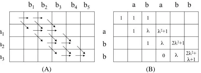
feature values. Since we are performing a depth-first traversal, we can accomplish the algorithm with a recursive function and do not have to store the full trie in memory. Figure 1 shows expansion down a path during the recursive traversal.
a b b a a a a a b a b a 1 2 1
a a a a a b a b a 2 4 3
a a a b b 5 0 0 0 a a a a a b a b a b b b b b b a b a b a b a b a a b a b a a b b 5
Figure 1: Trie traversal for gappy kernel. Expansion along a path from root to leaf during traveral of the trie for the (5,3)-gappy kernel, showing only the instance 5-mers for a single sequence x=abaabab. Each node stores its valid 5-mer instances and the index to the
last match for each instance. Instances at the leaf node contribute to the kernel for 3-mer feature abb.
The computation at the leaf node depends on which version of the gappy kernel one uses. For the unweighted feature map, we obtain the feature values of x and y corresponding to the current k-mer by counting the g-k-mer instances at the leaf coming from x and from y, respectively; the product of these counts gives the contribution to the kernel for this k-mer feature. For theλ-weighted gappy feature map, we need a count of all alignments of each valid g-mer instance against the k-mer feature allowing up to g−k gaps. This can be computed with a simple dynamic programming
routine (similar to the Needleman-Wunsch algorithm), where we sum over a restricted set of paths, as shown in Figure 2. The complexity is O(k(g−k)), since we fill a restricted trellis of(k+1)(g− k+1) squares. Note that when we align a subsequence bi1bi2. . .bik against a k-mer a1a2. . .ak, we
only penalize interior gaps corresponding to non-consecutive indices in 1≤i1<i2. . . <ik ≤g. Therefore, the multiplicative gap cost is 1 in the zeroth and last rows of the trellis andλin the other rows.
(A) (B)
Figure 2: Dynamic programming at the leaf node. The trellis in (A) shows the restricted paths for aligning a g-mer against a k-mer, with insertion of up to g−k gaps in the k-mer, for g=5 and k=3. The basic recursion for summing path weights is S(i,j) =m(ai,bj)S(i− 1,j−1) +g(i)S(i,j−1), where m(a,b) =1 if a and b match, 0 if they are different, and the gap penalty g(i) =1 for i=0,k and g(i) =λfor other rows. That is, except for the top and bottom rows, every time we move to the right, we introduce an additional internal gap and incur a multiplicative penalty ofλ; when we move diagonally, we see whether the corresponding characters match or not. Trellis (B) shows the example of aligning ababb against 3-mer abb. An explanation of how to interpret trellis diagrams for dynamic programming can be found in Durbin et al. (1998).
at the leaf nodes multiplied by the maximum number of times an instance is operated on as it is passed from root to leaf – plus the processing time at the leaf nodes need to compute the kernel
update. Each g-mer instance in the input data can contribute to
g k
k-mer features, which we can
write as O(gg−k)if g−k is smaller than k and O(gk)otherwise. For simplicity, we assume the more typical former case, and we let the reader make simple adjustments in the latter case. Therefore, at most O(gg−k(|x|+|y|)g-mer instances are processed at leaf nodes in the traversal. Since we iterate
through at most g positions of each g-mer instance as we pass from root to leaf, the traversal time is
O(gg−k+1(|x|+|y|)). The total processing time at leaf nodes is O(gg−k(|x|+|y|))for the unweighted gappy kernel and O(k(g−k)gg−k(|x|+|y|))for the weighted gappy kernel. Therefore, in both cases, we have total complexity of the form O(c(g,k)(|x|+|y|)), with c(g,k) =O((g−k)gg−k+1)for the more expensive kernel. Further discussion of the complexity argument and pseudocode for the algorithm can be found in Shawe-Taylor and Cristianini (2004).
3.2 (k,σ)-Substitution Kernel Computation
For the substitution kernel, computation is very similar to the mismatch kernel algorithm. We use a depth k trie to represent the feature space. We store, at each depth d node that we visit, a set of pointers to all k-mer instances α in the input data whose d-length prefixes have current mutation score −∑di=1log P(ai|bi)<σ of the current prefix pattern b1b2. . .bd, and we store the current mutation score for each k-mer instance. As we pass from a parent node at depth d to a child node at depth d+1 along a branch labeled with symbol b, we process each k-mer α by adding
−log P(ad+1|b) to the mutation score and pass it to the child if and only if the score is still less than σ. As before, we update the kernel at the leaf node by computing the contribution of the corresponding k-mer feature.
The number of leaf nodes visited in the traversal is O(Nσ(|x|+|y|)), where the constant is the maximum mutation neighborhood size, Nσ=maxα∈Σk|M(k,σ)|. We can chooseσsufficiently small
to get any desired bound on Nσ, but it is difficult to estimate how to set the parameters to obtain good SVM classification performance except by empirical results. Total complexity for the kernel value computation is O(kNσ(|x|+|y|)).
3.3 (k,m)-Wildcard Kernel Computation
Computation of the wildcard kernel is again very similar to the mismatch kernel algorithm. We use a depth k trie with branches labeled by characters inΣ∪{∗}, and we prune (do not traverse) subtrees corresponding to prefix patterns with greater than m wildcard characters. At each node of depth d, we maintain pointers to all k-mers instances in the input sequences whose d-length prefixes match the current d-length prefix pattern (with wildcards) represented by the path down from the root.
Each k-mer instance in the data matches at most ∑mi=0
k i
=O(km) k-length patterns having
up to m wildcards. Thus the number of leaf nodes visited is in the traversal is O(km(|x|+|y|)), and total complexity for the kernel value computation is O(km+1(|x|+|y|)).
3.4 Comparison with Mismatch Kernel Complexity
For the (k,m) mismatch kernel, the size of the mismatch neighborhood of an instance k-mer is
O(km|Σ|m), so total kernel value computation is O(km+1|Σ|m(|x|+|y|)). All the other kernels pre-sented here have running time O(cK(|x|+|y|)), where constant cKdepends on the parameters of the kernel but not on the size of the alphabetΣ. Therefore, we have improved constant term for larger alphabets (such as the alphabet of 20 amino acids). In Section 5, we show that these new, faster kernels have performance comparable to the mismatch kernel in protein classification experiments.
4. Transducer Representation
Cortes et al. (2002) recently showed that many known string kernels can be associated with and constructed from weighted finite state transducers with input alphabet Σ. We briefly outline their transducer formalism and give transducers for some of our newly defined kernels. For simplicity, we only describe transducers over the probability semiringR+= [0,∞), with regular addition and
multiplication.
Following the development in Cortes et al. (2002), a weighted finite state transducer overR+is
states I⊂Q, a set of output states F⊂Q, a finite set of transitions E⊂Q×(Σ∪ {ε})×(∆∪ {ε})×
R+×Q, an initial weight functionλ: I→R+, and a final weight functionρ: F→R+. Here, the
symbol εrepresents the empty string. The transducer can be represented by a weighted directed graph with nodes indexed by Q and each transition e∈E corresponding to a directed edge from its
origin state p[e]to its destination state n[e]and labeled by the input symbol i[e]it accepts, the output symbol o[e]it emits, and the weight w[e]it assigns. We write the label as i[e]: o[e]/w[e](abbreviated as i[e]: o[e]if the weight is 1).
For a pathπ=e1e2. . .ek of consecutive transitions (directed path in graph), the weight for the path is w[π] =w[e1]w[e2]. . .w[ek], and we denote p[π] =p[e1]and n[π] =n[ek]. We writeΣ∗=
∪k≥0Σk for the set of all strings over Σ. For an input string x∈Σ∗ and output string z∈∆∗, we denote by P(I,x,z,F) the set of paths from initial states I to final states F that accept string x and emit string z. A transducer T is called regulated if for any pair of input and output strings(x,z), the output weight[[T]](x,z)that T assigns to the pair is well-defined. The output weight is given by:
[[T]](x,z) =
∑
π∈P(I,x,z,F)
λ(p[π])w[π]ρ(n[π])
A key observation from Cortes et al. (2002) is that there is a general method for defining a string kernel from a weighted transducer T . Let Ψ:R+ →Rbe a semiring morphism (for us, it will
simply be inclusion), and denote by T−1the transducer obtained from T by transposing the input and output labels of each transition. Then if the composed transducer S=T◦T−1is regulated, one obtains a rational string kernel for alphabetΣvia
K(x,y) =Ψ([[S]](x,y)) =
∑
z
Ψ([[T]](x,z))Ψ([[T]](y,z))
where the sum is over all strings z∈∆∗(where∆is the output alphabet for T ) or equivalently, over all output strings that can be emitted by T . Therefore, we can think of T as defining a feature map indexed by all possible output strings z∈∆∗for T .
Using this construction, Cortes et al. showed that the k-gram counter transducer Tkcorresponds to the k-gram or k-spectrum kernel, and the gappy k-gram counter transducer Tk,λgives the
unre-stricted gappy k-gram kernel from Lodhi et al. (2002). Figure 3(a) shows the diagram of the 3-gram transducer T3, and Figure 3(b) gives the gappy 3-gram transducer T3,λ. Our(g,k,λ)-gappy kernel
K(Weighted Gapg,k,λ) can be obtained from the composed transducer T =Tk,λ◦Tg using the T◦T−1 con-struction. (In all our examples, we useλ(s) =1 for every initial state s andρ(t) =1 for every final state t.)
For the(k,m)-wildcard kernel, we set the output alphabet to be∆=Σ∪ {∗}and define a trans-ducer with m+1 final states, as indicated in the figure. The m+1 final states correspond to des-tinations of paths that emit k-grams with 0, 1, . . . , m wildcard characters, respectively. The(3,1) -wildcard transducer is shown in Figure 4.
(a)
(b)
Figure 3: The k-gram and gappy k-gram transducers. The diagrams show the 3-gram transducer (a) and the gappy 3-gram transducer (b) for a two-letter alphabet. Here, the edge label
a :ε:λ, for example, means “accept symbol a, output the empty symbolε, multiply the weight byλ”.
Figure 4: The(k,m)-wildcard transducer. The diagram shows the(3,1)-wildcard transducer for a two-letter alphabet.
5. Experiments
families. Protein domain sequences belonging to different families but the same superfamily are considered to be remote homologs in SCOP. In these experiments, remote homology is simulated by holding out all members of a target SCOP family from a given superfamily as a test set, while examples chosen from the remaining families in the same superfamily form the positive training set. The negative test and training examples are chosen from disjoint sets of folds outside the target family’s fold, so that negative test and negative training sets are unrelated to each other and to the positive examples. More details of the experimental set-up can be found in Jaakkola et al. (1999).
While in principle, we can define and test inexact matching string kernels for a wide range of parameters, in practice, only a small parameter range is biologically motivated for use in the remote protein homology detection problem. For the exact matching k-spectrum kernel (Leslie et al., 2002a), the only interesting parameter choices are k=3 and k=4, since exact occurrences of
k-mers of length k≥5 in remotely homologous proteins are so rare that the spectrum kernel would
mostly be 0 off the diagonal. By incorporating inexact matching such as mismatches or gaps, we can use slightly longer subsequence instances and allow a few mismatches or gaps; however, using very long subsequences, or allowing a great amount of mutation of subsequence instances in our inexact matching scheme, would not capture biologically realistic sequence similarity. For example, for the gappy kernel, we expect that length(g,k) = (6,4)– 4-mers allowing up to 2 gaps – would be a useful parameter choice, while allowing many more gaps and hence a longer g-length window would be less useful. We test a range of parameter choices that seem reasonable in the experiments below.
In the first and larger SCOP benchmark data set, based on SCOP version 1.37, we compare to the Fisher kernel of Jaakkola et al. (1999) in addition to our previous mismatch kernel. In the Fisher kernel method, the feature vectors are derived from profile HMMs trained on the positive training examples. The feature vector for sequence x is the gradient of the log likelihood function log P(x|θ)
defined by the model and evaluated at the maximum likelihood estimate for model parameters:
Φ(x) =∇θlog P(x|θ)|θ=θ0. The Fisher kernel was the best performing method on this data set prior
to the mismatch-SVM approach, whose performance is as good as Fisher-SVM and better than all other standard methods tried (Leslie et al., 2002b). We note that in this data set, additional positive training sequences were pulled in from the non-redundant protein sequence database using an iter-ative training method for the profile HMMs. The presence of these additional “domain homologs” makes the learning task easier for all methods.
We also include a second set of experiments to further investigate the dependence of SVM performance on parameter choices for the new kernels. This second data set is based on SCOP version 1.59 and contains only sequences from the SCOP database – no domain homologs are added. The experiments are similar to those described by Liao and Noble (2002) but use a more recent version of SCOP. In this data set, the positive training sets are quite small, and the learning task is more difficult in this setting. In particular, there is not enough positive training data to train profile HMMs in these experiments, so we do not report Fisher kernel results (which are not competitive in this setting).
There is another successful feature representation for protein classification, the SVM-pairwise method presented in Liao and Noble (2002). Here one uses an empirical kernel map based on pairwise Smith-Waterman (Waterman et al., 1991) alignment scores
where xi, i=1. . .m, are the training sequences and d(xi,x)is the E-value for the alignment score between x and xi. We have previously shown (Leslie et al., 2004) that the mismatch kernel used with an SVM classifier is competitive with SVM-pairwise on the SCOP benchmark presented in Liao and Noble (2002), so we do not repeat the SVM-pairwise experiments for the very similar benchmark here.
In both experiments, we normalized the kernel by k(x,y)← √ k(x,y)
k(x,x)√k(y,y). All methods are
eval-uated using the receiver operating characteristic (ROC) score, which is the area under the receiver operating curve, which plots the rate of true positives as a function of the rate of false positives as the threshold for the classifier varies (Gribskov and Robinson, 1996). Perfect ranking of all positives above all negatives gives an ROC score of 1, while a random classifier has an expected score close to 0.5. We also use the ROC-50 score, which is the normalized area under the receiver operating curve up to the first 50 false positives; this score focuses on the top of the ranking of the test examples produced by the classifier and is more informative when there are very few positive examples in the test set. Use of ROC-50 scores (or other ROC-N scores) is the most standard way of evaluating performance of homology detection methods in bioinformatics (Gribskov and Robinson, 1996).
Finally, we use kernel alignment scores (Cristianini et al., 2001) on the second SCOP data set to investigate the empirical differences between the different inexact matching models for protein sequence data, and we investigate methods for combining kernels to improve SVM performance.
5.1 SCOP Experiments with Domain Homologs: Comparison with Fisher and Mismatch Kernels
We first present experimental results for the new kernels on the larger of the two SCOP data sets, the Fisher-SCOP benchmark introduced by Jaakkola et al. (1999) that contains domain homologs for additional positive training data, and compare SVM classification performance to both the mismatch kernel and the Fisher kernel.
We tested the(g,k)-gappy kernel with parameter choices(g,k) = (6,4),(7,4),(8,5),(8,6), and
(9,6). Among them(g,k) = (6,4)yielded the best results, though other choices of parameters had quite similar performance (data not shown). We also tested the alternative weighted gappy kernel, where the contribution of an instance g-mer to a k-mer feature is a weighted sum of all the possible matches of the k-mer to subsequences in the g-mer with multiplicative gap penaltyλ(0<λ≤1). We used gap penaltyλ=1.0 andλ=0.5 with the(6,4)weighted gappy kernel. We found thatλ=0.5 weighting slightly weakened performance (results not shown). In Figure 5, we see that unweighted and weighted (λ=1.0) gappy kernels have comparable results to(5,1)-mismatch kernel and Fisher kernel.
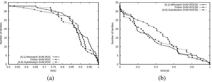
We tested the substitution kernels with(k,σ) = (4,6.0). Here,σ=6.0 was chosen so that the members of a mutation neighborhood of a particular 4-mer would typically have only one position with a substitution, and such substitutions would have fairly high probability. Therefore, the mu-tation neighborhoods were much smaller than, for example,(4,1)-mismatch neighborhoods. The results are shown in Figure 6. Again, the substitution kernel has comparable performance with mismatch-SVM and Fisher-SVM, though results are perhaps slightly weaker for more difficult test families.
In order to compare with the(5,1)-mismatch kernel, we tested wildcard kernels with parameters
0 5 10 15 20 25 30 35
0.5 0.55 0.6 0.65 0.7 0.75 0.8 0.85 0.9 0.95 1
Number of families
ROC (5,1)-Mismatch-SVM ROC Fisher-SVM ROC (6,4)-Gap-SVM(Weight=0.5) ROC (6,4)-Gap-SVM(Weight=1.0) ROC 0 5 10 15 20 25 30 35
0 0.2 0.4 0.6 0.8 1
Number of families
ROC50 (5,1)-Mismatch-SVM ROC50 Fisher-SVM ROC50 (6,4)-Gap-SVM(Weight=0.5) ROC50 (6,4)-Gap-SVM(Weight=1.0) ROC50 (a) (b)
Figure 5: Comparison of of Mismatch-SVM, Fisher-SVM and Gappy-SVM. The graph plots the total number of families for which a given method exceeds an ROC score threshold (a) or ROC-50 score threshold (b).
0 5 10 15 20 25 30 35
0.5 0.55 0.6 0.65 0.7 0.75 0.8 0.85 0.9 0.95 1
Number of families
ROC (5,1)-Mismatch-SVM ROC Fisher-SVM ROC (4,6)-Substitution-SVM ROC 0 5 10 15 20 25 30 35
0 0.2 0.4 0.6 0.8 1
Number of families
ROC50
(5,1)-Mismatch-SVM ROC50 Fisher-SVM ROC50 (4,6)-Substitution-SVM ROC50
(a) (b)
Figure 6: Comparison of mismatch-SVM, Fisher-SVM and substitution-SVM. The graph plots the total number of families for which a given method exceeds an ROC score threshold (a) or ROC-50 score threshold (b).
kernel, while enforcing a penalty on wildcard characters ofλ=0.5 seems to weaken performance somewhat.
If we compare results for the best-performing parameter choices that we tried from each kernel family – the (5,1)-mismatch kernel, the (5,1,1.0)-wildcard kernel, the (6,4)-gappy kernel with
λ=1.0, and the(4,6.0)-substitution kernel – then a signed ranked test with Bonferroni correction for multiple comparisons (Henikoff and Henikoff, 1992, Salzberg, 1997) and a p-value cut-off of 0.05 finds no significant differences between the four kernels, either on the basis of ROC or ROC-50 scores.
5.2 SCOP Experiments without Domain Homologs: Dependence on Parameters
0 5 10 15 20 25 30 35
0.5 0.55 0.6 0.65 0.7 0.75 0.8 0.85 0.9 0.95 1
Number of families
ROC (5,1)-Mismatch-SVM ROC Fisher-SVM ROC (5,1,1.0)-Wildcard-SVM ROC (5,1,0.5)-Wildcard-SVM ROC 0 5 10 15 20 25 30 35
0 0.2 0.4 0.6 0.8 1
Number of families
ROC50 (5,1)-Mismatch-SVM ROC50 Fisher-SVM ROC50 (5,1,1.0)-Wildcard-SVM ROC50 (5,1,0.5)-Wildcard-SVM ROC50 (a) (b)
Figure 7: Comparison of mismatch-SVM, Fisher-SVM and wildcard-SVM. The graph plots the total number of families for which a given method exceeds an ROC score threshold (a) or ROC-50 score threshold (b).
can explore how parameter choices affect SVM classification performance. We also use kernel alignment and kernel-target alignment scores (Cristianini et al., 2001) to investigate differences between different kernel models. Note that this data set contains no domain homologs, and thus the small amount of positive training data makes the experiments more difficult.
In experiments with the gappy kernel, we chose parameter values(g,k) = (6,4),(7,5)and(8,6)
and set the gap penalty toλ=1.0, the preferred choice from the previous experiments. The choice
(g,k) = (6,4)still produced the best classification results, which were slightly but not significantly weaker than those of (5,1)-mismatch kernel. The results are shown in Figure 8. Performance deteriorates as larger values of the g parameter are chosen with the number of gaps held fixed.
0 10 20 30 40 50 60
0.5 0.55 0.6 0.65 0.7 0.75 0.8 0.85 0.9 0.95 1
Number of families
ROC (5,1)-Mismatch-SVM ROC (6,4)-Gap-SVM(Weight=1.0) ROC Gap(5,7) Gap(6,8) 0 10 20 30 40 50 60
0 0.2 0.4 0.6 0.8 1
Number of families
ROC50
(5,1)-Mismatch-SVM ROC50 (6,4)-Gap-SVM(Weight=1.0) ROC50 (7,5)-Weight-Gap-SVM (Weight=1.0) ROC50 (8,6)-Weight-Gap-SVM (Weight=1.0) ROC50
(a) (b)
Figure 8: Dependence on parameters for the gappy kernel. The graph plots the total number of families for which a given method exceeds an ROC (a) or ROC-50 (b) score threshold.
as we vary k whileσis adjusted additively; however, as we see below, the Gram matrices produced by these different choices of kernels are in fact quite different.
0 10 20 30 40 50 60
0.5 0.6 0.7 0.8 0.9 1
No. of families with given performance
(6,9)-Substitution (5,1)-Mismatch-SVM ROC (4,6)-Substitution-SVM ROC (6,9)-Substitution 0 10 20 30 40 50 60
0 0.2 0.4 0.6 0.8 1
No. of families with given performance
(6,9)-Substitution-SVM ROC50 (5,1)-Mismatch-SVM ROC50 (4,6)-Substitution-SVM ROC50 (6,9)-Substitution-SVM ROC50
(a) (b)
Figure 9: Dependence on parameters for substitution kernel. The graph plots the total number of families for which a given method exceeds an ROC (a) or ROC-50 (b) score threshold. Results for three parameter choices give almost identical results.
We tested the wildcard kernel with(k,m,λ) = (5,1,1.0)and(5,2,1.0). We observed a signif-icant improvement in performance when we allowed up to 2 wildcards instead of 1 with k=5. The performance of(5,2,1.0)-wildcard kernel gave the best results among all kernel families and parameters that we tried, though several other kernel choices gave very similar performance. The re-sults are shown in Figure 10. Intuitively, it is clear that allowing 1 mismatch is closer to permitting 2 wildcards than to permitting a single wildcard: two k-mers that are identical except in two positions have intersecting (k,1)-mismatch neighborhoods and hence their (k,1)-mismatch feature vectors have non-zero inner product; similarly, such a pair of k-mers have non-orthogonal(k,2)-wildcard feature vectors but orthogonal(k,1)-wildcard feature vectors.
0 10 20 30 40 50 60
0.5 0.55 0.6 0.65 0.7 0.75 0.8 0.85 0.9 0.95 1
Number of families
ROC (5,1)-Mismatch-SVM ROC (5,1,1.0)-Wildcard-SVM ROC (5,2,1.0)-Wildcard-SVM ROC 0 10 20 30 40 50 60
0 0.2 0.4 0.6 0.8 1
Number of families
ROC50
(5,1)-Mismatch-SVM ROC50 (5,1,1.0)-Wildcard-SVM ROC50 (5,2,1.0)-Wildcard-SVM ROC50
(a) (b)
Kernel Kernel Alignment ROC ROC-50
(5,1)-mismatch 0.0982 0.875 0.416
(6,4)-gappy 0.1428 0.851 0.387
(7,5)-gappy 0.0269 0.825 0.315
(8,6)-gappy 0.0090 0.782 0.242
(4,6.0)-substitution 0.1643 0.876 0.441
(5,7.5)-substitution 0.0369 0.865 0.428
(6,9.0)-substitution 0.0170 0.871 0.442
(5,1,1.0)-wildcard 0.0310 0.816 0.304
(5,2,1.0)-wildcard 0.1565 0.881 0.447
Table 1: Mean ROC and ROC-50 scores over 54 target families.
Kernel (5,1)-mismatch (6,4)-gappy (4,6)-subst (6,9)-subst (5,1)-wildcard (5,2)-wildcard
(5,1)-mismatch 1.000 0.923 0.812 0.947 0.968 0.864
(6,4)-gappy 1.000 0.915 0.742 0.775 0.955
(4,6)-subst 1.000 0.591 0.622 0.942
(6,9)-subst 1.000 0.991 0.626
(5,1)-wildcard 1.000 0.669
(5,2)-wildcard 1.000
Table 2: Pairwise kernel alignment scores over the full SCOP data set.
In Table 1, we summarize the mean ROC and ROC-50 scores across the 54 target families for all the string kernels families and parameter values chosen. The table also shows mean training set kernel-target alignment scores across the experiments. Kernel alignment was introduced by Cristianini et al. (2001) as a measure of similarity between pairs of kernels or between a kernel and a target function. The empirical kernel alignment score between two kernels is defined as the value
hK1,K2i
p
hK1,K1ihK2,K2i
, where K1and K2are the Gram matrices for the kernels on the sample data, and
h·,·iis the euclidean inner product when the Gram matrices are viewed as vectors (Hilbert-Schmidt inner product). Thus the alignment score is simply the cosine of the angle between the two vectors representing Gram matrices. The empirical kernel-target alignment is the kernel alignment for a Gram matrix and the target yyt, where y is the column vector of labels.
Table 1 shows that for the gappy and wildcard kernels, high kernel-target alignment scores do seem to correlate with good SVM classification performance. However, for the substitution kernels, the kernel-target alignment is low for larger values of k while performance remains strong. In Table 2, we show the pairwise kernel alignment scores between normalized kernels on the full SCOP data set of 7329 sequences. In some cases, the alignment scores between kernels of the same family with different parameters can be quite low, for example the(5,1,1.0)-wildcard kernel and
Kernel ROC ROC-50
Keq(αi=1) 0.907 0.520
Kopt(σ=0.01) 0.901 0.502
Table 3: Mean ROC and ROC-50 scores of linearly combined kernels. Here Kopt =∑Ni=1αiKi, where N is the number of kernels, α is the optimal vector for the best alignment with target yy0, and the the regularization parameter depends onσas described in the text.
Since different kernels capture somewhat different notions of sequence similarity, we consider whether a convex combination of kernels K(α) =∑Ni=1αiKi, withαi≥0 for i=1. . .N, can outper-form individual kernels. We consider two schemes for choosing such a linear combination. In the first approach, we simply assign equal weightsαi =1/N for all i to obtain a new kernel Keq. For a second approach, we follow Kandola et al. (2002), who proposed a general method for learning theαi by solving a optimization problem to maximize the kernel alignment between Gram matrix of K(α)and target yy0,
A(S,K(α),yy0) = y0K(α)y
|y|||K(α)||,
yielding a new kernel Kopt. Here, one introduces a regularization parameterλto constrain||α||and prevent over-alignment; the optimization then amounts to a quadratic programming problem that can be solved through standard methods. We now pick 6 kernels with relatively good performance and low pairwise kernel alignment as components for the new kernel – (5,1)-mismatch, (6,4) -gappy,(4,6.0)-substitution,(5,7.5)-substitution,(6,9.0)-substitution and(5,2,1.0)-wildcard – and repeat the second set of SCOP experiments with these two linear combination kernels. For Kopt, we use a regularization parameter of the formλ=Nσ2∑i jhKi,Kji, whereh·,·iis the Hilbert-Schmidt inner product between matrices. We found that performance varied slightly but significantly as we varied σ=.001, .01, .1,1,10,100,1000 (results not shown); since the experiments do not contain a cross-validation set, we simply report the performance of the best parameter choice (σ=.01) with the caveat that this result may be somewhat optimistic. We report the mean ROC and ROC-50 scores across 54 experiments for the simple case Keq, and the optimal alignment case Kopt in Table 3. We found that Kopt with the best regularization parameter choice does achieve significant im-provement over the best individual kernel (indeed, almost all regularization parameters that we tried displayed some advantage over the best individual kernel); however, the simple weighting used in
Keqslightly outperformed Koptin these experiments. Interestingly, for most of 54 experiments, Kopt (σ=0.01) had non-zero weights only for the two best performing kernels, the(4,6.0)-substitution and(5,2,1.0)-wildcard kernels, with the weight for the latter about an order of magnitude smaller than that of the former. These results suggest that some of the kernels are complementary to each other and that combining them can help improve performance, though it appears that optimal align-ment does not outperform a simple uniform weighting scheme for combining kernels.
6. Discussion
new kernels, the time to compute a kernel value K(x,y)is O(cK(|x|+|y|)), where the constant cK depends on the parameters of the kernel but not on the size of the alphabetΣ. Thus we improve on the constant factor involved in computation of the previously presented mismatch kernel, in which
|Σ|as well as k and m control the size of the mismatch neighborhood and hence the constant cK. We also show how many of our kernels can be obtained through the recently presented trans-ducer formalism of rational T◦T−1 kernels and give the transducer T for several examples. This connection gives an intuitive understanding of the kernel definitions and could inspire new string kernels.
Finally, we present results on two benchmark SCOP data sets for the remote protein homology detection problem and show that many of the new, faster kernels achieve performance comparable to the mismatch kernel. We also investigate how kernel performance depends on parameter choice for the different inexact matching models. Intuitively, it is clear that the only biological reasonable choices involve short k-mer features, since as we allow k to grow, we cannot permit sufficient inexact matching without also introducing noise. However, within these constraints, our results demonstrate the somewhat different behavior of the various kernel families.
We note that Vishwanathan and Smola (2002) used counting statistics and a suffix tree con-struction to eliminate the constant factor of k in computation time for the exact-matching spectrum kernel (Leslie et al., 2002a). It may be possible to extend this technique to the fast inexact-matching kernels presented here.
A promising direction for applied work in this area is combining string kernel representations with semi-supervised approaches for leveraging the abundant unlabeled protein sequence data (se-quences whose 3D structure is unknown) available in sequence databases. One recent approach is presented by Weston et al. (2003), where string kernels are used as a base kernel representation, and unlabeled sequence data together with a dissimilarity measure between sequence examples are used to build cluster kernels that modify the base kernel for a richer representation. In more recent work (Kuang et al., 2004), we define k-mer based string kernels for probabilistic sequence profiles (Gribskov et al., 1987), which also give a richer representation of sequences by estimating posi-tion specific residue emission probabilities from unlabeled data. These profile-based string kernels provide another promising semi-supervised approach for kernel representation of protein sequence data.
Acknowledgments
We would like to thank Eleazar Eskin, Risi Kondor and William Stafford Noble for helpful dis-cussions and Corinna Cortes, Patrick Haffner and Mehryar Mohri for explaining their transducer formalism to us. This work is supported by an Award in Informatics from the PhRMA Foundation, NIH grant LM07276-02, and NSF grant ITR-0312706.
References
S. F. Altschul, W. Gish, W. Miller, E. W. Myers, and D. J. Lipman. A basic local alignment search tool. Journal of Molecular Biology, 215:403–410, 1990.
N. Cristianini and J. Shawe-Taylor. An Introduction to Support Vector Machines. Cambridge, 2000.
N. Cristianini, J. Shawe-Taylor, A. Elisseeff, and J. Kandola. On kernel-target alignment. In Neural
Information Processing Systems, volume 15, 2001.
R. Durbin, S. Eddy, A. Krogh, and G. Mitchison. Biological Sequence Analysis. Cambridge UP, 1998.
E. Eskin, W. S. Noble, Y. Singer, and S. Snir. A unified approach for sequence prediction using sparse sequence models. Technical report, Hebrew University, 2003.
M. Gribskov, A. D. McLachlan, and D. Eisenberg. Profile analysis: Detection of distantly related proteins. PNAS, pages 4355–4358, 1987.
M. Gribskov and N. L. Robinson. Use of receiver operating characteristic (ROC) analysis to evaluate sequence matching. Computers and Chemistry, 20(1):25–33, 1996.
D. Haussler. Convolution kernels on discrete structure. Technical report, UC Santa Cruz, 1999.
S. Henikoff and J. G. Henikoff. Amino acid substitution matrices from protein blocks. PNAS, 89: 10915–10919, 1992.
T. Jaakkola, M. Diekhans, and D. Haussler. Using the Fisher kernel method to detect remote protein homologies. In Proceedings of the Seventh International Conference on Intelligent Systems for
Molecular Biology, pages 149–158. AAAI Press, 1999.
J. Kandola, J. Shawe-Taylor, and N. Cristianini. Optimizing kernel alignment over combinations of kernels. NeoroCOLTTechnicalReport NC-TR-2002-121, http://www.neurocolt.org, 2002.
R. Kuang, E. Ie, K. Wang, K. Wang, M. Siddiqi, Y. Freund, and C. Leslie. Profile-based string kernels for remote homology detection and motif extraction. In Computational Systems
Bioinfor-matics, 2004.
C. Leslie, E. Eskin, A. Cohen, J. Weston, and W. S. Noble. Mismatch string kernels for discrimina-tive protein classification. Bioinformatics, 2004.
C. Leslie, E. Eskin, and W. S. Noble. The spectrum kernel: A string kernel for SVM protein classification. Proceedings of the Pacific Biocomputing Symposium, 2002a.
C. Leslie, E. Eskin, J. Weston, and W. S. Noble. Mismatch string kernels for SVM protein classifi-cation. Neural Information Processing Systems 16, 2002b.
C. Leslie and R. Kuang. Fast kernels for inexact string matching. Proceedings of COLT/Kernel
Workshop, 2003.
C. Liao and W. S. Noble. Combining pairwise sequence similarity and support vector machines for remote protein homology detection. Proceedings of the Sixth Annual International Conference
on Research in Computational Molecular Biology, 2002.
A. G. Murzin, S. E. Brenner, T. Hubbard, and C. Chothia. SCOP: A structural classification of proteins database for the investigation of sequences and structures. Journal of Molecular Biology, 247:536–540, 1995.
M. Sagot. Spelling approximate or repeated motifs using a suffix tree. Lecture Notes in Computer
Science, 1380:111–127, 1998.
S. L. Salzberg. On comparing classifiers: Pitfalls to avoid and a recommended approach. Data
Mining and Knowledge Discovery, 1:371–328, 1997.
R. M. Schwartz and M. O. Dayhoff. Matrices for detecing distant relationships. In Atlas of Protein
Sequence and Structure, pages 353–358, Silver Spring, MD, 1978. National Biomedical Research
Foundation.
J. Shawe-Taylor and N. Cristianini. Kernel Methods for Pattern Analysis. Cambridge University Press, 2004.
J.-P. Vert, H. Saigo, and T. Akutsu. Kernel Methods in Computational Biology, chapter Local alignment kernels for biological sequences. MIT Press, 2004.
S. V. N. Vishwanathan and A. Smola. Fast kernels for string and tree matching. Neural Information
Processing Systems 16, 2002.
M. S. Waterman, J. Joyce, and M. Eggert. Computer alignment of sequences, chapter Phylogenetic Analysis of DNA Sequences. Oxford, 1991.
C. Watkins. Dynamic alignment kernels. Technical report, UL Royal Holloway, 1999.