Learning with Decision Lists of Data-Dependent Features

Learning with Decision Lists of Data-Dependent Features

Mario Marchand MARIO.MARCHAND@IFT.ULAVAL.CA

D´epartement IFT-GLO Universit´e Laval

Qu´ebec, Canada, G1K-7P4

Marina Sokolova SOKOLOVA@SITE.UOTTAWA.CA

School of Information Technology and Engineering University of Ottawa

Ottawa, Ontario K1N-6N5, Canada

Editor: Manfred K. Warmuth

Abstract

We present a learning algorithm for decision lists which allows features that are constructed from the data and allows a trade-off between accuracy and complexity. We provide bounds on the gen-eralization error of this learning algorithm in terms of the number of errors and the size of the classifier it finds on the training data. We also compare its performance on some natural data sets with the set covering machine and the support vector machine. Furthermore, we show that the proposed bounds on the generalization error provide effective guides for model selection.

Keywords: decision list machines, set covering machines, sparsity, data-dependent features,

sam-ple compression, model selection, learning theory

1. Introduction

The set covering machine (SCM) has recently been proposed by Marchand and Shawe-Taylor (2001, 2002) as an alternative to the support vector machine (SVM) when the objective is to obtain a sparse classifier with good generalization. Given a feature space, the SCM attempts to find the smallest conjunction (or disjunction) of features that gives a small training error. In contrast, the SVM attempts to find the maximum soft-margin separating hyperplane on all the features. Hence, the two learning machines are fundamentally different in what they are aiming to achieve on the training data.

To investigate if it is worthwhile to consider larger classes of functions than just the conjunctions and disjunctions that are used in the SCM, we focus here on the class of decision lists (Rivest, 1987) because this class strictly includes both conjunctions and disjunctions while being strictly included in the class of linear threshold functions (Ehrenfeucht and Haussler, 1989; Blum and Singh, 1990; Marchand and Golea, 1993).

proposed an attribute efficient algorithm that outputs a decision list of O(rklogkm) attributes for a training set of m examples where k denotes the number of alternations of the target decision list (see the definition in Section 2). However, both of these algorithms are unattractive for the practitioner because they do not provide an accuracy-complexity tradeoff. Indeed, real-world data are often noisy and, therefore, simpler functions that make some training errors might be better than more complex functions that make no training errors. Since the amount of noise is problem-specific, a learning algorithm should provide to the user a means to control the tradeoff between accuracy and the complexity of a classifier. Ideally, the user should be able to choose from a wide range of functions that includes very simple functions (like constants), that almost always underfit the data, and very complex functions that often overfit the data. But this latter requirement for decision lists can be generally achieved only if the set of features used for the decision list is data-dependent. It is only with a data-dependent set of features that a restricted class of functions like decision lists can almost always overfit any training data set (that does not contain too many pairs of identical examples with opposite classification labels). Hence, in this paper, we present a learning algorithm for decision lists which can be used with any set of features, including those that are defined with respect to the training data, and that provides some “model selection parameters” (also called learning parameters) for allowing the user to choose the proper tradeoff between accuracy and complexity.

We denote by decision list machine (DLM) any classifier which computes a decision list of Boolean-valued features, including features that are possibly constructed from the data. In this paper, we use the set of features known as data-dependent balls (Marchand and Shawe-Taylor, 2001; Sokolova et al., 2003) and the set of features known as data-dependent half-spaces (Marchand et al., 2003). We show, on some natural data sets, that the DLM can provide better generalization than the SCM with the same set of features.

We will see that the proposed learning algorithm for the DLM with data-dependent features is effectively compressing the training data into a small subset of examples which is called the

compression set. Hence, we will show that the DLM with data-dependent features is an example

of a sample-compression algorithm and we will thus propose a general risk bound that depends on the number of examples that are used in the final classifier and the size of the information message needed to identify the final classifier from the compression set. The proposed bound will apply to any compression set-dependent distribution of messages (see the definition in Section 4) and allows for the message set to be of variable size (in contrast with the sample compression bound of Littlestone and Warmuth (1986) that requires fixed size). We will apply this general risk bound to DLMs by making appropriate choices for a compression set-dependent distribution of messages and we will show, on natural data sets, that these specialized risk bounds are generally slightly more effective than K-fold cross validation for selecting a good DLM model.

This paper extends the previous preliminary results of Sokolova et al. (2003).

2. The Decision List Machine

Let x denote an arbitrary n-dimensional vector of the input space

X

which is an arbitrary subset of Rn_{. We consider binary classification problems for which the training set S=P∪N consists of a}

features. Given that subset

R

, and an arbitrary input vector x, the output f(x)of the decision list machine (DLM) is given by the following rule

If (h1(x)) then b1

Else If (h2(x)) then b2 . . .

Else If (hr(x)) then br

Else br+1,

where each bi∈ {0,1}defines the output of f(x)if and only if hiis the first feature to be satisfied on x (i.e. the smallest i for which hi(x) =1). The constant br+1(where r=|

R

|) is known as the default

value. Note that f computes a disjunction of the his whenever bi=1 for i=1. . .r and br+1=0. To compute a conjunction of his, we simply place in f the negation of each hiwith bi=0 for i=1. . .r

and br+1=1. Note, however, that a DLM f that contains one or many alternations (i.e. a pair (bi,bi+1)for which bi6=bi+1for i<r) cannot be represented as a (pure) conjunction or disjunction of his (and their negations). Hence, the class of decision lists strictly includes conjunctions and

disjunctions.

We can also easily verify that decision lists are a proper subset of linear threshold functions in the following way. Given a DLM with r features as above, we assign a weight value wito each hiin

the DLM in order to satisfy

|wi_|> r

∑

j=i+1

|wj| ∀i∈ {1, . . . ,r}.

Let us satisfy these constraints with_|wi|=2r−ifor i∈ {1, . . . ,r}. Then, for each i, we set wi= +|wi|

if bi=1, otherwise we set wi=−|wi|if bi=0. For the thresholdθwe useθ=−1/2 if br+1=1 andθ= +1/2 if br+1=0. With this prescription, given any example x, we always have that

sgn

r

∑

i=1

wihi(x)−θ

!

= 2bk−1,

where k is the smallest integer for which hk(x) =1 in the DLM or k=r+1 if hi(x) =0 ∀i∈

{1, . . . ,r_}. Hence, with this prescription, the output of the linear threshold function is the same as the output of the DLM for all input x. Finally, to show that the subset is proper we simply point out that a majority vote of three features is a particular case of a linear threshold function that cannot be represented as a decision list since the output of the majority vote cannot be determined from the value of a single feature.

From our definition of the DLM, it seems natural to use the following greedy algorithm for building a DLM from a training set. For a given set S0=P0_∪N0 of examples (where P0_⊆P and N0_⊆N) and a given set

H

of features, consider only the features hi∈

H

which either have hi(x) =0

for all x_∈P0 or hi(x) =0 for all x∈N0. Let Qi be the subset of examples on which hi=1 (our

constraint on the choice of hi implies that Qi contains only examples having the same class label).

We say that hi is covering Qi. The greedy algorithm starts with S0=S and an empty DLM. Then

it finds a hi with the largest|Qi|and appends(hi,b)to the DLM (where b is the class label of the

either P0or N0is empty. It finally assigns br+1to the class label of the remaining non-empty set of examples.

Following Rivest (1987), this greedy algorithm is assured to build a DLM that makes no training errors whenever there exists a DLM on a set

E

_⊆

H

of features that makes zero training errors. However, this constraint is not really required in practice since we do want to permit the user of a learning algorithm to control the tradeoff between the accuracy achieved on the training data and the complexity (here the size) of the classifier. Indeed, a small DLM which makes a few errors on the training set might give better generalization than a larger DLM (with more features) which makes zero training errors. One way to include this flexibility is to early-stop the greedy algorithm when there remains a few more training examples to be covered. But a further reduction in the size of the DLM can be accomplished by considering features hi that cover examples of both classes.

Indeed, if Qidenotes the subset of S0on which hi=1 (as before), let Pidenote the subset of P0that

belongs to Qi and let Ni be the subset of N0 that belongs to Qi (thus Qi=Pi∪Ni). In the previous

greedy algorithm, we were considering only features hifor which either Pi or Ni was empty. Now

we are willing to consider features for which neither Pi nor Niis empty whenever max(|Pi|,|Ni|)is

substantially larger than before. In other words, we want now to consider features that may err on a few examples whenever they can cover many more examples. We therefore define the usefulness Ui

of feature hi by

Ui

def

= max_{|Pi| −pn|Ni|,|Ni| −pp|Pi|},

where pn denotes the penalty of making an error on a negative example whereas pp denotes the

penalty of making an error on a positive example. Indeed, whenever we add to a DLM a feature hi

for which Pi and Ni are both non empty, the output biassociated with hiwill be 1 if|Pi| −pn|Ni| ≥

|Ni_{| −}pp_|Pi|or 0 otherwise. Hence, the DLM will necessarily incorrectly classify the examples in Niif bi=1 or the examples in Piif bi=0.

Hence, to include this flexibility in choosing the proper tradeoff between complexity and accu-racy, each greedy step will be modified as follows. For a given training set S0=P0_∪N0, we will select a feature hiwith the largest value of Uiand append(hi,1)to the DLM if|Pi|−pn|Ni| ≥ |Ni|−pp|Pi|,

otherwise, we append (hi,0) to the DLM. If (hi,1) was appended, we will then remove from S0 every example in Pi (since they are correctly classified by the current DLM) and we will also

re-move from S0every example in Ni (since a DLM with this feature is already misclassifying Ni, and,

consequently, the training error of the DLM will not increase if later features err on the examples in Ni). Similarly if(hi,0)was appended, we will then remove from S0the examples in Qi=Ni∪Pi.

Hence, we recover the simple greedy algorithm when pp=pn=∞.

The formal description of our learning algorithm is presented in Figure 1. Note that we always set br+1=¬brsince, otherwise, we could remove the rth feature without changing the classifier’s

output f for any input x.

The penalty parameters pp and pnand the early stopping point s of BuildDLM are the

Algorithm BuildDLM(S,pp,pn,s,

H

)

Input: A set S of examples, the penalty values pp and pn, a stopping point s, and a set

H

=_{hi(x)}| H_|

i=1of Boolean-valued features.

Output: A decision list f consisting of an ordered set

R

=_{(hi,bi)_}r

i=1 of features hi with their corresponding output values bi, and a default value br+1.

Initialization:

R

=/0, r=0,S0=S,b0=¬a (where a is the label of the majority class).

1. For each hi∈

H

, let Qi =Pi∪Ni be the subset of S0 for which hi =1 (where Pi consists of

positive examples and Niconsists of negative examples). For each hi compute Ui, where:

Uidef= max_{|Pi_{| −}pn_|Ni_|, _|Ni_{| −}pp_|Pi_|}

2. Let hk be a feature with the largest value of Uk. If Qk = /0 then go to step 6 (no progress

possible).

3. If (|Pk| −pn|Nk| ≥ |Nk| −pp|Pk|) then append(hk,1)to

R

. Else append(hk,0)to

R

.

4. Let S0=S0₋Qkand let r=r+1.

5. If (r<s and S0contains examples of both classes) then go to step 1

6. Set br+1=¬br. Return f .

Figure 1: The learning algorithm for the decision list machine

The time complexity of BuildDLM is trivially bounded as follows. Assuming a time of at most

t for evaluating one feature on one example, it takes a time of at most_|

H

_|mt to find the first feature

of the DLM for a training set of m examples. For the data-dependent set of features presented in Section 3.1, it is (almost) always possible to find a feature that covers at least one example. In that case, it takes a time of O(_|

H

_|mst)to find s features. Note that the algorithm must stop if, at some greedy step, there does not exists a feature that covers at least one training example.

Generally, we can further reduce the size of the DLM by observing that any feature hi with bi =br+1 can be deleted from the DLM if there does not exist a training example x with label

y=br+1 and another feature hj with j>i and bj=6 bi for which hi(x) =hj(x) =1 (since, in that

case, feature hi can be moved to the end of the DLM without changing the output for any correctly

classified training example). The algorithm PruneDLM of Figure 2 deletes all such nodes from the DLM.

We typically use both algorithms in the following way. Given a training set, we first run

Build-DLM without early stopping (i.e., with parameter s set to infinity) to generate what we call a plate DLM. Then we consider all the possible DLMs that can be obtained by truncating this

Algorithm PruneDLM(S,f)

Input: A set S of examples, a decision list f consisting of an ordered set

R

=_{(hi,bi)_}r i=1 of features hiwith their corresponding output values bi, and a default value br+1.

Output: The same decision list f with, possibly, some features removed.

Initialization: l=r

1. Let(hk,bk)_∈

R

be the pair with the largest value of k such that bk=br+1and k<l.

2. If (@(hj,bj)∈

R

: j>k, bj 6=bk, hj(x) =hk(x)for some (x,y)∈S with y=br+1) then delete(hk,bk)from

R

.

3. l=k.

4. If (l>1) then go to step 1; else stop.

Figure 2: The pruning algorithm for the decision list machine

the DLM that contains the first two features, and so on, up to the DLM that contains all r features. Then we run PruneDLM on all these DLMs to try to reduce them further. Finally all these DLMs are tested on a provided testing set.

It is quite easy to build artificial data sets for which PruneDLM decreases substantially the size of the DLM. However, for the natural data sets used in Section 7, PruneDLM almost never deleted any node from the DLM returned by BuildDLM.

3. Data-Dependent Features

The set of data-dependent balls (Marchand and Shawe-Taylor, 2001) and data-dependent

half-spaces (Marchand et al., 2003) were introduced for their usage with the SCM. We now need to

adapt their definitions for using them with the DLM.

3.1 Balls and Holes

Let d :

X

2_{→Rbe a metric for our input space}

_X

_{. Let h}

c,ρbe a feature identified by a center c and a radiusρ. Feature hc,ρis said to be a ball iff hc,ρ(x) =1∀x : d(x,c)≤ρand 0 otherwise. Similarly,

feature hc,ρis said to be a hole iff hc,ρ(x) =1∀x : d(x,c)>ρand 0 otherwise. Hence, a ball is a

feature that covers the examples that are located inside the ball; whereas a hole covers the examples that are located outside. In general, both types of features will be used in the DLM.

Partly to avoid computational difficulties, we are going to restrict the centers of balls and holes to belong to the training set, i.e., each center c must be chosen among_{xi:(xi,yi)∈S}for a given

training set S. Moreover, given a center c, the set of relevant radius values are given by the positions of the other training examples, i.e., the relevant radius values belong to _{d(c,xi):(xi,yi)∈S}.

effectively compressing the training data into the smaller set of examples used for its features. This is the other reason why we have constrained the centers and radii to these values. Hence, given a training set S of m examples, the set

H

of features used by the DLM will contain O(m2) balls and holes. This is a data-dependent set of features since the features are defined with respect to the training data S.

Whenever a ball (or hole) hc,ρis chosen to be appended to the DLM, we must also provide an

output value b which will be the output of the DLM on example x when hc,ρis the first feature of

the DLM that has hc,ρ(x) =1. In this paper we always choose b to be the class label of c if hc,ρis

a ball. If hc,ρis a hole, then we always choose b to be the negation of the class label of c. We have

not explored the possibility of using balls and holes with an output not given by the class label of its center because, as we will see later, this would have required an additional information bit in order to reconstruct the ball (or hole) from its center and border and, consequently, would have given a looser generalization error bound without providing additional discriminative power (i.e., power to fit the data) that seemed “natural”.

To avoid having examples directly on the decision surface of the DLM, the radiusρof a ball of center c will always be given byρ=d(c,b)₋εfor some training example b chosen for the border and some fixed and very small positive value ε. Similarly, the radius of a hole of center c will always be given byρ=d(c,b) +ε. We have not chosen to assign the radius values “in between” two training example since this would have required three examples per ball and hole and would have decreased substantially the tightness of our generalization error bound without providing a significant increase of discriminative power.

With these choices for centers and radii, it is straightforward to see that, for any penalty values

ppand pn, the set of balls having the largest usefulness U always contains a ball with a center and

border of opposite class labels whereas the set of holes having the largest usefulness always contains a hole having a center and border of the same class label. Hence, we will only consider such balls and holes in the set of features for the DLM. For a training set of mp positive examples and mn

negative examples we have exactly 2mpmn such balls and m2p+m2nsuch holes. We thus provide to BuildDLM a set

H

of at most(mp+mn)2_features.

Finally, note that this set of features has the property that there always exists a DLM of these features that correctly classifies all the training set S provided that S does not contain a pair of contradictory examples, i.e.,(x,y)and(x0,y0)such that x=x0 and y₆=y0. Therefore, this feature set gives to the user the ability to choose the proper tradeoff between training accuracy and function size.

3.2 Half-Spaces

With the use of kernels, each input vector x is implicitly mapped into a high-dimensional vector φφφ(x)such thatφφφ(x)_·φφφ(x0) =k(x,x0)(the kernel trick). We consider the case where each feature is a half-space constructed from a set of 3 points_{φφφ_a,φφφ_b,φφφ_c}where eachφφφ_l is the image of an input example xltaken from the training set S. We consider the case where xaand xbhave opposite class

labels and the class label of xc is the same as the class label of xb. The weight vector w of such a

half-space hc_a,b is defined by wdef=φφφ_a−φφφ_b and its threshold t by tdef=w_·φφφ_c+εwhereε is a small positive real number. We useε>0 to avoid having examples directly on the decision surface of the DLM. Hence

where

t=k(xa,xc)−k(xb,xc) +ε.

Whenever a half-space hc_a,b is chosen to be appended to the DLM, we must also provide an output value b which will be the output of the DLM on example x when hc_a,bis the first feature of the DLM having hc_a,b(x) =1. From our definition above, we choose b to be the class label ofφφφ_a. Hence, a DLM made of these three-example features is effectively compressing the training set into the smaller set of examples used for its features.

Given a training set S of m=mp+mnexamples, the set

H

of features considered by the DLM will contain at most m_·mp_·mnhalf-spaces. However, in contrast with the set of balls and holes, we are not guaranteed to always be able to cover all the training set S with these half-spaces.

Finally, note that this set of features (in the linear kernel case k(x,x0) =x_·x0) was already proposed by Hinton and Revow (1996) for decision tree learning but no formal analysis of their learning method has been given.

4. A Sample Compression Risk Bound

Since our learning algorithm tries to build a DLM with the smallest number of data-dependent fea-tures, and since each feature is described in terms of small number of training examples (two for balls and holes and three for half-spaces), we can thus think of our learning algorithm as compress-ing the traincompress-ing set into a small subset of examples that we call the compression set.

Hence, in this section, we provide a general risk bound that depends on the number of examples that are used in the final classifier and the size of the information message needed to identify the final classifier from the compression set. Such a risk bound was first obtained by Littlestone and Warmuth (1986). The bound provided here allows the message set to be of variable size (whereas previous bounds require fixed size). In the next section, we will compare this bound with other well known bounds. Later, we apply this general risk bound to DLMs by making appropriate choices for a compression set-dependent distribution of messages. Finally, we will show, on natural data sets, that these specialized risk bounds provide an effective guide for choosing the model-selection parameters of BuildDLM.

Recall that we consider binary classification problems where the input space

X

consists of an

arbitrary subset ofRn and the output space

Y

=_{0,1}. An example zdef= (x,y)is an input-output pair where x_∈

X

and y_∈

Y

. We are interested in learning algorithms that have the following prop-erty. Given a training set S=_{z1, . . . ,zm}of m examples, the classifier A(S)returned by algorithm A is described entirely by two complementary sources of information: a subset zi of S, called the

compression set, and a message stringσwhich represents the additional information needed to ob-tain a classifier from the compression set zi. This implies that there exists a reconstruction function

R

, associated to A, that outputs a classifier

R

(σ,zi)when given an arbitrary compression set ziand

message stringσchosen from the set

M

(zi)of all distinct messages that can be supplied to

R

with

the compression set zi. It is only when such an

R

exists that the classifier returned by A(S)is always

identified by a compression set ziand a message stringσ.

Given a training set S, the compression set zi is defined by a vector i of indices such that

i def= (i1,i2, . . . ,i_|i|) (1)

with : ij∈ {1, . . . ,m} ∀j

where|i|denotes the number of indices present in i.

The classical perceptron learning rule and support vector machines are examples of learning algorithms where the final classifier can be reconstructed solely from a compression set (Graepel et al., 2000, 2001). In contrast, we will see in the next section that the reconstruction function for DLMs needs both a compression set and a message string.

We seek a tight risk bound for arbitrary reconstruction functions that holds uniformly for all compression sets and message strings. For this, we adopt the PAC setting where each example z is drawn according to a fixed, but unknown, probability distribution D on

X

_×

Y

. The risk R(f)of any classifier f is defined as the probability that it misclassifies an example drawn according to D:

R(f)def=Pr_(x,y)∼D(f(x)₆=y) =E_(x,y)∼DI(f(x)₆=y),

where I(a) =1 if predicate a is true and 0 otherwise. Given a training set S=_{z1, . . . ,zm}of m

examples, the empirical risk RS(f)on S, of any classifier f , is defined according to

RS(f)

def = 1

m m

∑

i=1

I(f(xi)6=yi)

def

=E₍x,y)∼SI(f(x)6=y).

Let Zm denote the collection of m random variables whose instantiation gives a training sample

S=zm=_{z1, . . . ,zm}. Let us denote PrZm_∼Dm(·)by P_Zm(·). The basic method to find a bound on

the true risk of a learning algorithm A, is to bound P0where

P0 def= PZm(R(A(Zm))>ε). (2)

Our goal is to find the smallest value forεsuch that P0_≤δsince, in that case, we have

PZm(R(A(Zm))≤ε)≥1−δ.

Recall that classifier A(zm) is described entirely in terms of a compression set zi⊂zm and a

message stringσ_∈

M

(zi). Let

I

be the set of all 2mvectors of indices i as defined by Equation 1.

Let

M

(zi)be the set of all messagesσthat can be attached to compression set zi. We assume that

the empty message is always present in

M

(zi) so that we always have |

M

(zi)| ≥1. Since any

i_∈

I

andσ_∈

M

(zi)could a priori be reached by classifier A(zm), we bound P0 by the following

probability

P0 _≤ PZm(∃i∈

I

:∃σ∈

M

(Z_i): R(

R

(σ,Z_i))>ε) def= P00,

where Zi are the random variables whose instantiation gives zi and whereεdepends on Zi,σand

the amount of training errors. In the sequel, we denote by i the vector of indices made of all the indices not present in i. Since PZm(·) =E_Z

iPZ_i|Zi(·), we have (by the union bound)

P00 ≤

∑

i∈I

EZiPZ_i|Zi(∃σ∈

M

(Zi): R(

R

(σ,Zi))>ε)

≤

∑

i∈I

EZi

∑

σ∈M(Zi)

PZ_i|Zi(R(

R

(σ,Zi))>ε). (3)

We will now stratify PZ_i|Zi(R(

R

(σ,Zi))>ε)in terms of the errors that

R

(σ,Zi)can make on

indices where each index is not present in i. Given a training sample zmand a compression set zi,

we denote by Rz_i(f)the vector of indices pointing to the examples in z_i which are misclassified by

f . We have

PZ_i|Zi(R(

R

(σ,Zi))>ε)) =

∑

j∈Ii

PZ_i|Zi R(

R

(σ,Zi))>ε,RZi(

R

(σ,Zi)) =j

. (4)

But now, since the classifier

R

(σ,Zi)is fixed when(σ,Zi)is fixed, and since each Ziis independent

and identically distributed according to the same (but unknown) distribution D, we have

PZ_i|Zi R(

R

(σ,Zi))>ε,RZi(

R

(σ,Zi)) =j

≤(1₋ε)m−|i|−|j|. (5)

Hence, by using Equations 3, 4, and 5, we have

P00 _≤

∑

i∈Ij

∑

∈Ii

EZi

∑

σ∈M(Zi)

[1₋ε(σ,Zi,j)]m−|i|−|j|, (6)

where we have now shown explicitly the dependence ofεon Zi,σ, and j.

Given any compression set zi, let us now use any function PM(zi)(σ)which has the property that

∑

σ∈M(zi)

PM(zi)(σ)≤1 (7)

and can, therefore, be interpreted as compression set-dependent distribution of messages when it sums to one. Let us then chooseεsuch that

m

|i_|

m− |i| |j_|

[1₋ε(σ,Zi,|j|)]m−|i|−|j|=PM(Zi)(σ)·ζ(|i|)·ζ(|j|)·δ, (8)

where, for any non-negative integer a, we define

ζ(a)def= 6

π2(a+1)−

2_{. (9)}

In that case, we have indeed that P0 _≤δsince∑∞_i=1i−2=π2_{/6. Any choice forζ(a) is allowed as} long as it is a non negative function who’s sum is bounded by 1.

The solution to Equation 8 is given by

ε(σ,Zi,|j|,δ) = 1−exp −

1

m_{− |}i_{| − |}j_|

"

ln

m

|i_|

+ln

m− |i| |j_|

+ln 1

PM(Zi)(σ)

!

+

ln

1 ζ(_|i_|)ζ(_|j_|)δ

. (10)

We have therefore shown the following theorem:

Theorem 1 For any δ_∈(0,1]and for any sample compression learning algorithm with a recon-struction function

R

that maps arbitrary subsets of a training set and information messages to classifiers, we have

Although the risk bound given by Theorem 1 (and Equation 10) increases with the amount|j| of training errors made on the examples that do not belong to the compression set zi, it is interesting

to note that it is independent of the amount of errors made on the compression set. However, a reconstruction function will generally need less additional information when it is constrained to produce a classifier making no errors with the compression set. Hence, the above risk bound will generally be smaller for sample-compression learning algorithms that always return a classifier making no errors on the compression set. But this constraint might, in turn, force the learner to produce classifiers with larger compression sets.

Finally note that the risk bound is small for classifiers making a small number_|j_|of training er-rors, having a small compression set size_|i_|, and having a message stringσwith large prior “proba-bility” PM(Zi)(σ). This “probability” is usually larger for short message strings since larger message

strings are usually much more numerous at sharing the same “piece” (or fraction) of probability.

5. Comparison with Other Risk Bounds

Although the risk bound of Theorem 1 is basically a sample compression bound it, nevertheless, applies to a much broader class of learning algorithms than just sample compression learning al-gorithms. Indeed the risk bound depends on two complementary sources of information used to identify the classifier: the sample compression set zi and the message stringσ. In fact, the bound

still holds when the sample compression set vanishes and when the classifier h=

R

(σ)is described entirely in terms of a message string σ. It is therefore worthwhile to compare the risk bound of Theorem 1 to other well-known bounds.

5.1 Comparison with Data-Independent Bounds

The risk bound of Theorem 1 can be qualified as “data-dependent” when the learning algorithm is searching among a class of functions (classifiers) described in terms of a subset zi of the training

set. Nevertheless, the bound still holds when the class of functions is “data-independent” and when individual functions of this class are identified only in terms of a (data-independent) messageσ. In that limit,_|i_|=0 and the risk boundεdepends only onσand the number_|j_|=k of training errors:

ε(σ,k,δ) =1−exp

−1

m₋k

ln

m k

+ln

1

PM(σ)

+ln

1 ζ(k)δ

. (11)

Since here each classifier h is given by

R

(σ)for someσ_∈

M

, we can consider

M

as defining a data-independent set of classifiers. This set may contain infinitely many classifiers but it must be countable. Indeed all that is required is

∑

σ∈M

P(σ)_≤1

for any fixed prior P over

M

. If we further restrict the learning algorithm to produce a classifier that always make no training errors (k=0) and if we choose P(σ) =1/_|

M

_{| ∀}σ_∈

M

for some finite set

M

, we obtain the famous Occam’s razor bound (Blumer et al., 1987)

ε(δ) =1₋exp

−1

m

ln

|

M

_|

δ

≤_m1

ln

|

M

_|

δ

where we have used 1−exp(₋x)_≤x. Hence the bound of Equation 11 is a generalization of the

Occam’s razor bound to the case of an arbitrary (but fixed) prior P(σ) over a countably infinite set

M

of classifiers which are possibly making some training errors. Consequently, the bound of Theorem 1 is a generalization of the Occam’s razor bound to the case where the classifiers are identified by two complementary sources of information: the message stringσand the compression set zi.

The proposed bound is obtained by using a union bound over the possible compression subsets of the training set and over the possible messagesσ_∈

M

(zi). This bound therefore fails when we

consider a continuous set of classifiers. In view of the fact that the set of DLMs of data-dependent features is a subset of the same class of functions but with features that are not constrained to be identified by pairs or triples of training examples, why not use the well-known Vapnik-Chervonenkis (VC) bounds (Vapnik, 1998) or Rademacher bounds (Mendelson, 2002) to characterize the learn-ing algorithms discussed in this paper? The reason is that the proposed algorithms are indeed constrained to use a data-dependent set of features identified by pairs and triples of training exam-ples. The risk bound of Theorem 1 therefore reflects more the set of possible classifiers that can be produced by the proposed algorithms than the VC or Rademacher bounds which are suited for algorithms that can produce any classifier of a continuous set.

5.2 Comparison with Other Sample Compression Risk Bounds

The risk bound of Theorem 1 can be reduced to the sample compression bounds of Littlestone and Warmuth (1986) if we perform the following changes and specializations:

• We restrict the set

M

of possible messages to be a finite set which is the same for all possible compression sets zi.

• For the distribution of messages, we use1

PM(σ) =

1

|

M

_| ∀σ∈

M

.

• Theorem 1 is valid for any functionζthat satisfies ∑m_i=0ζ(i)_≤1. Here we will useζ(a) = 1/(m+1) _∀a_{∈ {}0, . . . ,m_}. This choice increases the bound since 6π−2_(a+1)−2_>1/(m+ 1)for a<p6(m+1)/π₋1.

• We use the approximation 1₋exp(₋x)_≤x to obtain a looser (but somewhat easier to

under-stand) bound.

With these restrictions and changes we obtain the following bounds for_|j_|=0 and_|j_{| ≥}0:

ε(_|i|,δ) _≤ 1

m_{− |}i_|

ln

m

|i_|

+ln

|

M

_|

δ

+ln(m+1)

for|j|=0, (13)

ε(_|i_|,_|j_|,δ) _≤ 1

m_{− |}i_{| − |}j_|

ln

m

|i_|

+ln

m_{− |}i_| |j_|

+

ln

|

M

_|

δ

+2 ln(m+1)

for_|j_{| ≥}0. (14)

Apart from the ln(m+1)terms, these bounds are the same as the sample compression bounds of Lit-tlestone and Warmuth (1986). The ln(m+1) terms are absent from the Littlestone and Warmuth compression bounds because their bounds hold uniformly for all compression sets of a fixed size |i|and for all configurations of training error points of a fixed amount |j|. A ln(m+1) term oc-curs in the bound of Equation 13 from the extra requirement to hold uniformly for all compression set sizes. Still an extra ln(m+1)term occurs in Equation 14 from the extra requirement to hold uniformly for all amounts_|j_|of training errors. The bound of Theorem 1 holds uniformly for all compression sets of arbitrary sizes and for all configurations of training error points of an arbitrary amount. But instead of using ζ(a) =1/(m+1) _∀a_{∈ {}0, . . . ,m_}we have used the tighter form given by Equation 9.

It is also interesting to compare the bounds of Equations 13 and 14 with the sample compression bounds given by Theorems 5.17 and 5.18 of Herbrich (2002). The bound of Equation 13 is the same as the bound of Theorem 5.17 of Herbrich (2002) when_|

M

_|=1 (no messages used). When the classifier is allowed to make training errors, the bound of Equation 14 is tighter than the lossy compression bound of Theorem 5.18 of Herbrich (2002) when_|j_| m since the latter have used the

Hoeffding inequality which becomes tight only when_|j_|is close to m/2.

Consequently, the bound of Theorem 1 is tighter than the above-mentioned sample compression bounds for three reasons. First, the approximation 1₋exp(₋x)_≤x was not performed. Second, the

functionζ(a)of Equation 9 was used instead of the looser factor of 1/(m+1). Third, in contrast with the other sample compression bounds, the bound of Theorem 1 is valid for any a priori defined sample compression-dependent distribution of messages PM(zi)(σ).

This last characteristic may be the most important contribution of Theorem 1. Indeed, we feel that it is important to allow the set of possible messages and the message set size to depend on the sample compression zisince the class labels of the compression set examples give information

about the set of possible data-dependent features that can be constructed from zi. Indeed, it is

conceivable that for some zi, very little extra information may be needed to identify the classifier

whereas for some other zi, more information may be needed. Consider, for example, the case

where the compression set consists of two examples that are used by the reconstruction function

R

to obtain a single-ball classifier. For the reconstruction function of the set covering machine (described in the next section), a ball border must be a positive example whereas both positive and negative examples are allowed for ball centers. In that case, if the two examples in the compression set have a positive label, the reconstruction function needs a message string of at least one bit that indicates which example is the ball center. If the two examples have opposite class labels, then the negative example is necessarily the ball center and no message at all is needed to reconstruct the classifier. More generally, the set of messages that we use for all types of DLMs proposed in this paper depends on some properties of zi like its number n(zi)of negative examples. Without such a

dependency on zi, the set of possible messages

M

could be unnecessarily too large and would then

loosen the risk bound.

5.3 Comparison with the Set Covering Machine Risk Bound

to obtain a classifier, it partitions the compression set into three disjoint sets. Hence, we cannot compare directly the bound of Theorem 1 with the SCM risk bound since the latter is much more specialized than the former. Instead we will show how we can apply the general risk bound of Theorem 1 to the case of the SCM just by choosing an appropriate sample compression-dependent distribution of messages PM(zi)(σ).

Recall that the task of the SCM is to construct the smallest possible conjunction of (Boolean-valued) features. We discuss here only the conjunction case. The disjunction case is treated similarly just by exchanging the role of the positive with the negative examples.

For the case of data-dependent balls and holes, each feature is identified by a training example called a center(xc,yc), and another training example called a border(xb,yb). Given any metric d,

the output h(x)on any input example x of such a feature is given by

h(x) =

yc if d(x,xc)≤d(x,xb)

¬yc otherwise.

In this case, given a compression set zi, we need to specify the examples in zi that are used for a

border point without being used as a center. As explained by Marchand and Shawe-Taylor (2001), no additional amount of information is required to pair each center with its border point whenever the reconstruction function

R

is constrained to produce a classifier that always correctly classifies the compression set. Furthermore, as argued by Marchand and Shawe-Taylor (2001), we can limit ourselves to the case where each border point is a positive example. In that case, each message σ∈

M

(zi)just needs to specify the positive examples that are a border point without being a center.

Let n(zi)and p(zi)be, respectively, the number of negative and the number of positive examples in

compression set zi. Let b(σ)be the number of border point examples specified in messageσand let

ζ(a)be defined by Equation 9. We can then use

PM(Zi)(σ) =ζ(b(σ))·

p(zi)

b(σ)

−1

(15)

since, in that case, we have for any compression set zi:

∑

σ∈M(zi)

PM(zi)(σ) = p(zi)

∑

b=0

ζ(b)

∑

σ:b(σ)=b

p(zi)

b(σ)

−1

≤1.

With this distribution PM(zi), the risk bound of Theorem 1 specializes to

ε(σ,Zi,|j|,δ) = 1−exp

−1

m_{− |}i_{| − |}j_|

ln

m

|i_|

+ln

m_{− |}i_| |j_|

+ln

p(zi)

b(σ)

+

ln

1

ζ(_|i_|)ζ(_|j_|)ζ(b(σ))δ

. (16)

In contrast, the SCM risk bound of Marchand and Shawe-Taylor (2001) is equal to

ε0_(σ,Z

i,|j|,δ) = 1−exp

−1

m_{− |}i_{| − |}j_|

ln

m

|i_|

+ln

m_{− |}i_| |j_|

+

ln

cp(zi) +cn(zi) +b(zi)

cp(zi)

+ln

m2_|i_|

δ

where cp(zi) and cn(zi) denote, respectively, the number of positive centers and the number of

negative centers in ziand where b(zi)denotes the the number of borders in zi.

Hence, we observe only two differences between these two bounds. First, the (larger) ln(m2_|i_|/δ) term of Marchand and Shawe-Taylor (2001) has been replaced by the (smaller) ln(1/ζ(_|i|)ζ(_|j|)ζ(b(σ))δ) term. Second, the coefficient

cp(zi) +cn(zi) +b(zi)

cp(zi)

has been replaced by the smaller coefficient

p(zi)

b(σ)

.

We can verify that this last coefficient is indeed smaller since

p(zi)

b(σ)

=

cp(zi) +b(zi)

b(zi)

=

cp(zi) +b(zi)

cp(zi)

≤

cp(zi) +cn(zi) +b(zi)

cp(zi)

.

Consequently, the risk bound of Theorem 1, applied to the SCM with the distribution given by Equation 15, is smaller than the SCM risk bound of Marchand and Shawe-Taylor (2001).

6. Risks Bounds for Decision List Machines

To apply the risk bound of Theorem 1, we need to define a distribution of message strings2PM(zi)(σ)

for each type of DLM that we will consider. Once that distribution is known, we only need to insert it in Equation 10 to obtain the risk bound. Note that the risk bound does not depend on how we actually code σ(for some receiver, in a communication setting). It only depends on the a priori probabilities assigned to each possible realization ofσ.

6.1 DLMs Containing Only Balls

Even in this simplest case, the compression set zi alone does not contain enough information to

identify a DLM classifier (the hypothesis). To identify unambiguously the hypothesis we need to provide also a message stringσ.

Recall that, in this case, zicontains ball centers and border points. By construction, each center

is always correctly classified by the hypothesis. Moreover, each center can only be the center of one ball since the center is removed from the data when a ball is added to the DLM. But a center can be the border of a previous ball in the DLM and a border can be the border of more than one ball (since the border of a ball is not removed from the data when that ball is added to the DLM). Hence, σneeds to specify the border points in zi that are a border without being the center of another ball.

Letσ1be the part of the message stringσthat will specify that information and let P1(σ1) be the probabilities that we assign to each possible realization of σ1. Since we expect that most of the compression sets will contain roughly the same number of centers and borders, we assign, to each example of zi, an equal a priori probability to be a center or a border. Hence we use

P1(σ1) = 1

2|i| ∀σ1.

2. We will refer to P_M(zi)as the “distribution” of messages even though its summation over the possible realizations of

Onceσ1is specified, the centers and borders of zi are identified. But to identify each ball we

need to pair each center with a border point (which could possibly be the center of another ball). For this operation, recall that the border and the center of each ball must have opposite class labels. Letσ2 be the part of the message stringσthat specifies that pairing information and let P2(σ2|σ1) be the probabilities that we assign to each possible realization ofσ2onceσ1is given. Let n(zi)and

p(zi)be, respectively, the number of negative and the number of positive examples in compression

set zi. Consider now a positive center example x of zi. Since a border point can be used for more

that one ball and a center can also be used as a border, we assign an equal probability of 1/n(zi)

to each negative example of zi to be paired with x. Similarly, we assign an equal probability of

1/p(zi) to each positive example to be paired with a negative center of zi. Let cp(zi) and cn(zi)

be, respectively, the number of positive centers and negative centers in zi(this is known onceσ1is specified). For an arbitrary compression set zi, we thus assign the following a priori probability to

each possible pairing information stringσ2:

P2(σ2|σ1) =

1

n(zi)

cp(zi)

1

p(zi)

cn(zi)

∀σ2|n(zi)6=0 and p(zi)6= 0.

This probability is, indeed, correctly defined only under the condition that n(zi)6=0 and p(zi)6=0.

However, since the border and center of each ball must have opposite labels, this condition is the same as_|i_{| 6}=0. When_|i_|=0, we can just assign 1 to P2(σ2|σ1). By using the indicator function

I(a)defined previously, we can thus write P2(σ2|σ1)more generally as

P2(σ2|σ1) =

1

n(zi)

cp(zi)

1

p(zi)

cn(zi)

I(_|i_{| 6}=0) + I(_|i_|=0) _∀σ2.

Onceσ1andσ2 are known, each ball of the DLM is known. However, to place these balls in the DLM, we need to specify their order. Let r(zi)

def

=cp(zi) +cn(zi)be the number of balls in the

DLM (this is known onceσ1andσ2are specified). Letσ3be the part of the message stringσthat specifies this ordering information and let P3(σ3|σ2,σ1)be the probabilities that we assign to each possible realization ofσ3 onceσ1andσ2are given. For an arbitrary compression set zi, we assign

an equal a priori probability to each possible ball ordering by using

P3(σ3|σ2,σ1) = 1

r(zi)! ∀

σ3.

The distribution of messages is then given by P1(σ1)P2(σ2|σ1)P3(σ3|σ2,σ1). Hence

PM(zi)(σ) =

1 2|i|·

"

1

n(zi)

cp(zi)

1

p(zi)

cn(zi)

I(_|i_{| 6}=0) + I(_|i_|=0)

#

·_r(z1

i)! ∀

σ. (18)

6.2 DLMs Containing Balls and Holes

set zi could be used for two holes: giving a total of|i|(|i| −1) features. The first part σ1 of the (complete) message stringσwill specify the number r(zi)of features present in compression set zi.

Since we always have r(zi)<|i|2for|i|>0, we could give equal a priori probability for each value

of r∈ {0, . . . ,_|i|2}. However since we want to give a slight preference to smaller DLMs, we choose to assign a probability equal toζ(r)(defined by Equation 9) for all possible values of r. Hence

P1(σ1) =ζ(r(zi)) ∀σ1.

The second partσ2ofσspecifies, for each feature, if the feature is a ball or a hole. For this, we give equal probability to each of the r(zi)features to be a ball or a hole. Hence

P2(σ2|σ1) =2−r(zi) ∀σ2.

Finally, the third partσ3ofσspecifies, sequentially for each feature, the center and border point. For this, we give an equal probability of 1/_|i_| to each example in zi of being chosen (whenever

|i_{| 6}=0). Consequently

P3(σ3|σ2,σ1) =|i|−2r(zi)I(|i| 6=0) +I(|i|=0) ∀σ3.

The distribution of messages is then given by P1(σ1)P2(σ2|σ1)P3(σ3|σ2,σ1). Hence

PM(zi)(σ) =ζ(r(zi))·2

−r(zi)_·

h

|i_|−2r(zi)_{I(|i| 6=0) +I(|i|=0)}i _∀σ_{. (19)}

6.3 Constrained DLMs Containing Only Balls

A constrained DLM is a DLM that has the property of correctly classifying each example of its compression set ziwith the exception of the compression set examples who’s output is determined

by the default value. This implies that BuildDLM must be modified to ensure that this constraint is satisfied. This is achieved by considering, at each greedy step, only the features hi with an output biand covering set Qithat satisfy the following property. Every training example(x,y)∈Qithat is

either a border point of a previous feature (ball or hole) in the DLM or a center of a previous hole in the DLM must have y=biand thus be correctly classified by hi.

We will see that this constraint will enable us to provide less information to the reconstruction function (to identify a classifier) and will thus yield tighter risk bounds. However, this constraint might, in turn, force BuildDLM to produce classifiers containing more features. Hence, we do not know a priori which version will produce classifiers having a smaller risk.

Let us first describe the simpler case where only balls are permitted.

As before, we use a string σ1, with the same probability P1(σ1) =2−|i| ∀σ1to specify if each example of the compression set ziis a center or a border point. This gives us the set of centers which

coincides with the set of balls since each center can only be used once for this type of DLM. Next we use a string σ2 to specify the ordering of each center (or ball) in the DLM. As before we assign equal a priori probability to each possible ordering. Hence P2(σ2|σ1) =1/r(zi)! ∀σ2 where r(zi)denotes the number of balls for zi (an information given byσ1).

But now, since each feature was constrained to correctly classify the examples of zithat it covers

examples in zi. We start with P0=P,N0=N and do the following, sequentially, from the first center

(or ball) to the last. If center c is positive, then its border b is given by argmin_x∈N0d(c,x)and we

remove from P0 (to find the border of the other balls) the center c and all other positive examples covered by that feature and used by the previous features. If center c is negative, then its border b is given by argmin_x∈P0d(c,x)and we remove from N0 the center c and all other negative examples

covered by that feature and used by the previous features. The distribution of messages is then given by

PM(zi)(σ) =

1 2|i|·

1

r(zi)! ∀

σ. (20)

6.4 Constrained DLMs Containing Balls and Holes

As for the case of Section 6.2, we use a stringσ1to specify the number r(zi)of features present in

compression set zi. We also use a stringσ2 to specify, for each feature, if the feature is a ball or a hole. The probabilities P1(σ1)and P2(σ2|σ1)used are the same as those defined in Section 6.2. Here, however, we only need to specify the center of each feature, since, as we will see below, no additional information is needed to find the border of each feature when the DLM is constrained to classify correctly each example in zi. Consequently

PM(zi)(σ) =ζ(r(zi))·2

−r(zi)_·

h

|i|−r(zi)_{I(|i| 6=0) +I(|i|=0)}i _∀σ_{. (21)}

To specify the border of each feature, we use the following algorithm. Given a compression set zi, let P and N denote, respectively, the set of positive and the set of negative examples in zi.

We start with P0=P,N0_{=N and do the following, sequentially, from the first feature to the last. If} the feature is a ball with a positive center c, then its border is given by argmin_x∈N0d(c,x)and we

remove from P0 the center c and all other positive examples covered by that feature and used by the previous features. If the feature is a hole with a positive center c, then its border is given by argmax_x∈P0_−{c}d(c,x)and we remove from N0all the negative examples covered by that feature and

used by the previous features. If the feature is a ball with a negative center c, then its border is given by argmin_x∈P0d(c,x)and we remove from N0 the center c and all other negative examples covered

by that feature and used by the previous features. If the feature is a hole with a negative center c, then its border is given by argmax_x∈N0_−{c}d(c,x)and we remove from P0 all the positive examples

covered by that feature and used by the previous features.

6.5 Constrained DLMs with Half-Spaces

Recall that each half-space is specified by weight vector w and a threshold value t. The weight vector is identified by a pair(xa,xb)of examples having opposite class labels and the threshold is

specified by a third example xcof the same class label as example xa.

The first part of the message will be a stringσ1 that specifies the number r(zi) of half-spaces

used in the compression set zi. As before, let p(zi) and n(zi) denote, respectively, the number

of positive examples and the number of negative examples in the compression set zi. Let P(zi)

and N(zi) denote, respectively, the set of positive examples and the set of negative examples in

the compression set zi. From these definitions, each pair (xa,xb)∈P(zi)×N(zi)∪N(zi)×P(zi)

having the same weight vector w must have a different threshold since, otherwise, they would cover the same set of examples. Hence the total number of half-spaces in the DLM is at most_|i_|p(zi)n(zi).

Therefore, for the stringσ1that specifies the number r(zi)of half-spaces used in the compression set

zi, we could assign the same probability to each number between zero and|i|p(zi)n(zi). However,

as before, we want to give preference to DLMs having a smaller number of half-spaces. Hence we choose to assign a probability equal to ζ(r) (defined by Equation 9) for all possible values of r. Therefore

P1(σ1) =ζ(r(zi)) ∀σ1.

Next, the second part σ2 of σ specifies, sequentially for each half-space, the pair (xa,xb)∈ P(zi)×N(zi)∪N(zi)×P(zi)used for its weight vector w. For this we assign an equal probability

of 1/2p(zi)n(zi)for each possible w of each half-space. Hence

P2(σ2|σ1) =

1 2p(zi)n(zi)

r(zi)

∀σ2|n(zi)6=0 and p(zi)6=0.

The condition that n(zi)6=0 and p(zi)6=0 is equivalent to|i| 6=0 since, for any half-space, xaand xbmust have opposite labels. Hence, more generally, we have

P2(σ2|σ1) =

1 2p(zi)n(zi)

r(zi)

I(_|i_{| 6}=0) + I(_|i_|=0) _∀σ2.

Finally, as for the other constrained DLMs, we do not need any additional message string to identify the threshold point xc∈zifor each w of the DLM. Indeed, for this task we can perform the following

algorithm. Let P and N denote, respectively, the set of positive and the set of negative examples in zi.

We start with P0=P,N0=N and do the following, sequentially, from the first half-space to the last.

Let w=φφφ(xa)−φφφ(xb)be the weight vector of the current half-space. If xa∈P then, for the threshold

point xc, we choose xc=argmax

x∈N0

w_·x and we remove from P0the positive examples covered by this

half-space and used by the previous half-spaces. Else if xa∈N then, for the threshold point xc, we

choose xc=argmax

x∈P0

w_·x and we remove from N0the negative examples covered by this half-space

and used by the previous half-spaces.

Consequently, the distribution of message strings is given by

PM(zi)(σ) =ζ(r(zi))·

"

1 2p(zi)n(zi)

r(zi)

I(_|i_{| 6}=0) + I(_|i_|=0)

#

∀σ. (22)

6.6 Unconstrained DLMs with Half-Spaces

As for the case of Section 6.5, we use a stringσ1to specify the number r(zi)of half-spaces present

in compression set zi. We also use a stringσ2 to specify, sequentially for each half-space, the pair (xa,xb)∈P(zi)×N(zi)∪N(zi)×P(zi)used for its weight vector w. Hence, the probabilities P1(σ1)

and P2(σ2|σ1)used are the same as those defined in Section 6.5. But here, in addition, we need to specify the threshold point xc for each w. For this, we give an equal probability of 1/|i|to each

example in zi of being chosen (when|i| 6=0). Consequently, the distribution of messages is given

by

PM(zi)(σ) =ζ(r(zi))·

"

1 2p(zi)n(zi)

r(zi)

|i_|−r(zi)_I(

|i_{| 6}=0) + I(_|i_|=0)

#

7. Empirical Results on Natural Data

We have tested the DLM on several “natural” data sets which were obtained from the machine learning repository at UCI. For each data set, we have removed all examples that contained attributes with unknown values and we have removed examples with contradictory labels (this occurred only for a few examples in the Haberman data set). The remaining number of examples for each data set is reported in Table 3. No other preprocessing of the data (such as scaling) was performed. For all these data sets, we have used the 10-fold cross-validation error as an estimate of the generalization error. The values reported are expressed as the total number of errors (i.e. the sum of errors over all testing sets). We have ensured that each training set and each testing set, used in the 10-fold cross validation process, was the same for each learning machine (i.e. each machine was trained on the same training sets and tested on the same testing sets).

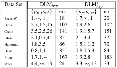
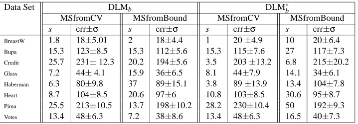
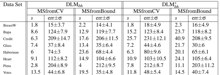
Table 1 and Table 2 show the DLM sizes s and penalty values that gave the smallest 10-fold cross-validation error separately for the following types of DLMs that we have studied in Section 6:

DLMb: unconstrained DLMs with balls (only).

DLM∗_b: constrained DLMs with balls (only).

DLMbh: unconstrained DLMs with balls and holes.

DLM∗_bh: constrained DLMs with balls and holes.

DLMhsp: unconstrained DLMs with half-spaces.

DLM∗_hsp: constrained DLMs with half-spaces.

For each of these DLMs, the learning algorithm used was BuildDLM. We have observed that

PruneDLM had no effect on all these data sets, except for Credit where it was sometimes able to

remove one feature.

In Table 3, we have compared the performance of the DLM with the set covering machine (SCM) using the same sets of data-dependent features, and the support vector machine (SVM) equipped with a radial basis function kernel of variance 1/γand a soft-margin parameter C.

We have used the L2metric for the data-dependent features for both DLMs and SCMs to obtain a fair comparison with SVMs. Indeed, the argument of the radial basis function kernel is given by the L2metric between two input vectors. For the SVM, the values of s refer to the average number of support vectors obtained from the 10 different training sets of 10-fold cross-validation. For the SCM, the value of T indicates the type of features it used and whether the SCM was a conjunction (c) or a disjunction (d). The values of p and s for the SCM refer to the penalty value and the number of features that gave the smallest 10-fold cross-validation error. We emphasize that, for all learning machines, the values of the learning parameters reported in Tables 1, 2, and 3 are the ones that gave the smallest 10-fold cross-validation error when chosen among a very large list of values. Although this overestimates the performance of every learning algorithm, it was used here to compare equally fairly (or equally unfairly) every learning machine. We will report below the results for DLMs when the testing sets are not used to determine the best values of the learning parameters.