Lyapunov Design for Safe Reinforcement Learning

Lyapunov Design for Safe Reinforcement Learning

Theodore J. Perkins [email protected]

Andrew G. Barto [email protected]

Department of Computer Science University of Massachusetts Amherst Amherst, MA 01003, USA

Editors: Carla E. Brodley and Andrea Danyluk

Abstract

Lyapunov design methods are used widely in control engineering to design controllers that achieve qualitative objectives, such as stabilizing a system or maintaining a system’s state in a desired operating range. We propose a method for constructing safe, reliable reinforcement learning agents based on Lyapunov design principles. In our approach, an agent learns to control a system by switching among a number of given, base-level controllers. These controllers are designed using Lyapunov domain knowledge so that any switching policy is safe and enjoys basic performance guarantees. Our approach thus ensures qualitatively satisfactory agent behavior for virtually any reinforcement learning algorithm and at all times, including while the agent is learning and taking exploratory actions. We demonstrate the process of designing safe agents for four different control problems. In simulation experiments, we find that our theoretically motivated designs also enjoy a number of practical benefits, including reasonable performance initially and throughout learning, and accelerated learning.

Keywords: Reinforcement Learning, Lyapunov Functions, Safety, Stability

1. Introduction

ac-tions and learning errors cease to threaten the agent’s performance. However, one still may not know if the behavior that the agent has learned is safe and successful in all possible situations. Depending on the precise criteria used, this may be difficult or impossible (undecidable) to determine.

Safety and reliability have always been important issues in control engineering. Often, the problems studied in control engineering are not formulated as optimal control problems. Commonly stated goals for controlling a system include: stabilizing a system around some operating point, tracking a desired system trajectory, or keeping the system’s state in some range (see, for example, Sontag, 1990; Levine, 1996; and Vincent and Grantham, 1997, for general treatments and Craig, 1989, for a discussion of robotics problems in particular). For a number of individual problems and abstract classes of problems, provably correct solutions have been developed for achieving qualitative goals such as these. Of course, the number of problems that have yielded to analysis is not as large as one would like. And in implementing such a solution, one must worry about whether the real system to be controlled behaves enough like the abstract problem that the solution is valid. Still, analytical solutions to qualitative formulations of control problems have been invaluable in a wide array of disciplines, including robotics, networking, and numerous branches of engineering.

In this paper we show that by using qualitative control technologies in a reinforcement learn-ing framework, one can design qualitatively safe and reliable agents that can learn approximate solutions to optimal control problems. We find that appropriate use of qualitative domain knowl-edge greatly improves the initial performance of a learning system; ensures reasonable performance throughout learning; and extends the range of problems that can reasonably be solved to include, for example, problems requiring high-precision control.

The primary qualitative technique we use is Lyapunov control design. Lyapunov functions are a fundamental tool used in control theory, and other disciplines, for studying the stability of systems evolving through time. Intuitively, a Lyapunov function is a scalar function of the system state on which system trajectories descend monotonically. Often, a Lyapunov function is thought of as a kind of “energy” which the system continually dissipates. In physical systems, a Lyapunov function may correspond to some real, natural notion of energy. For example, a ball rolling on a horizontal plane subject to friction is continually sapped of its kinetic energy, slowing the ball down. A mechanical wristwatch winds down as the potential energy stored in its spring is expended in driving the motion of the hands. In other cases, a Lyapunov function may be more abstract, such as an error or distance measure between the system state and a desired system state or trajectory. A Lyapunov function can be viewed as a form of domain knowledge that qualitatively describes certain aspects of the dynamics of the system. We know, for example, that the rolling ball and the wristwatch will eventually slow to a halt, though we may not know precisely where or when.

The notion of a control Lyapunov function generalizes the Lyapunov function concept to sys-tems that receive control inputs. A control Lyapunov function is a scalar function of the system state on which some control inputs cause trajectories that descend. Intuitively, our main proposal is to achieve safe, reliable reinforcement learning control by constraining the action choices of the agent so that all actions cause the system to descend on an appropriate control Lyapunov function. Qualitative performance guarantees follow directly from the descent constraint. We do not need to make any assumptions about the internals of the learning agent. It may be actively learning to con-trol the system, choosing actions randomly, or simply executing a previously-learned policy. Thus, our approach is consistent with virtually any choice of reinforcement learning algorithm.

to problems in which the agent’s task is to optimally bring the state of its environment to some region of state space, possibly a goal region, to maintain the state there, or to cause the state to follow some desired path. For a given optimal control problem of one of these types, finding an appropriate Lyapunov function may not be an easy task. Further, it may be that in restricting the agent to behave in ways that are provably qualitatively satisfactory, we may be ruling out other qualitatively satisfactory behaviors that are superior according to the cost function of the optimal control problem. Nevertheless, we expect that when Lyapunov domain knowledge is available, the theoretical assurances we gain and the ability to readily solve new classes of problems will outweigh such drawbacks.

In Section 2 we define the Markov decision process framework that we use to formulate optimal control problems. We also describe a number of qualitative safety and reliability properties that can be established using Lyapunov-based action constraints. Section 3 begins with background on Lya-punov functions and concludes with definitions and theorems necessary for establishing qualitative system properties. Following this is a sequence of four example problems in which we demon-strate Lyapunov analysis, demondemon-strate the process of designing learning agents based on Lyapunov domain knowledge, and present empirical evaluations of learning both with and without Lyapunov domain knowledge. In Section 7 we describe related work, and in Section 8 we conclude and discuss directions for future work.

2. Markov Decision Processes and Qualitative Solution Properties

We model the agent’s environment as a Markov decision process (MDP), evolving on an arbitrary state set S. The state of the environment at time t∈ {0,1,2,...}is denoted by st. The initial state, s0, is determined according to an initial state distribution S0(or probability measure, if one prefers). At each time t, the agent chooses an action, at, from the set of allowed actions, A(st). The immediate cost incurred, ct ∈R, and the next state of the environment, st₊1∈S, are determined stochastically according to a joint distribution depending on the state-action pair(st,at).

In some MDPs there is a set of goal states, G⊂S. When the environment enters a goal state, the

agent incurs a terminal cost but no further costs are incurred and no further actions are taken. As far as the optimal control problem is concerned, we say that the trial, or trajectory, ends once a goal state is reached. However, real systems do not necessarily stop once a goal state is reached. For example, once a robot arm is moved to a goal configuration, we may consider the optimal control task to be completed. However, in practice we may be concerned with whether the arm stays in the goal configuration. In our demonstration problems, and for the qualitative properties described below, it is sometimes useful to consider what happens to the system after it reaches a goal state.

A stochastic policy π maps each state s∈S to a distribution over A(s). The expected (un)-discounted return of policyπis defined to be

Vπ= lim τ→∞E

(

τ

∑

γt_c t

)

,

In general, we cannot expect a reinforcement learning controller to obtain an optimal or even near optimal policy to an optimal control problem. During learning, suboptimal behavior is a given. Yet in some settings, it may be important for us to ensure reasonable performance at all times. For example, we may want to know that excessive costs will not be incurred or that safety constraints will not be violated. Below, we define a number of qualitative system properties that can be used to express safety or performance objectives.

Let T ⊂S. One of the simplest questions we may ask is, “Does the agent keep the environment

in set T , if it starts there?” If T is taken to be a set of “safe” states, then this property can be used to express a safety constraint that we want the controller to satisfy. Such a property may hold for all possible trajectories of the system, or for a probability one1set of system trajectories.

Property 1 (Remain in T ) For certain/with probability 1, if s0∈T , then for all t ∈ {1,2,...},

st ∈T .

Another natural question is, “Does the controller cause the system to enter T from any initial state?” When T =G, this property expresses a guarantee of goal achievement.

Property 2 (Reach T ) For certain/with probability 1, there exists t≥0 such that st ∈T .

Combining the two previous properties expresses the property that the agent is guaranteed to bring the environment to a part of state space and keep it there.

Property 3 (Reach and remain in T ) For certain/with probability 1, there existsτ∈ {0,1,2,...}

such that for all t≥τ, st ∈T .

For some MDPs it is impossible to maintain the state in a given set T . A less restrictive requirement is that the environment spend an infinite amount of time in T —always returning to T if it leaves.

Property 4 (Infinite time in T ) For certain/with probability 1, for infinitely many distinct t ∈

{0,1,2,...}, st ∈T .

The final property we describe is convergence to T . For this we require a distance-to-T function

δT : S→R+. At the least, this function should satisfyδT(s) =0 for s∈T andδT(s)>0 for s∈/T . Property 5 (Converge to T ) For certain/with probability 1, limt→∞δT(st) =0.

Questions such as the first four are often addressed in the model-checking literature. Indeed, Gordon (2000) has demonstrated the relevance of model-checking techniques for verifying learning systems. In her approach, policy changes recommended by a learning component of an agent are verified for safety by a model-checking component. Only if the changes are safe are they imple-mented. Model-checking techniques are most successful in finite-state domains. It remains to be seen whether such approaches can be usefully applied to the continuous, infinite state-set problems upon which we focus.

Property 5 is often studied in control theory, typically taking T to contain a single state. Since our MDP framework allows for problems with infinite state sets, all of these properties are unde-cidable. (See Blondel and Tsitsiklis, 2000, for a survey of complexity results from a control theory perspective. Interestingly, even quite innocent-looking finite-dimensional continuous-state systems can implement Turing machine computations.) Our situation differs from the usual control theory setting because of the presence of the learning agent acting on the system. Nevertheless, control-theoretic techniques can be useful in establishing the qualitative properties listed above.

3. Lyapunov Functions and Design

Lyapunov’s so-called “second” method was originally proposed as a tool for studying the stability of systems of differential equations. The central task is to identify a Lyapunov function for the system—a scalar function of the system’s state with negative derivative along system trajectories. Identifying a Lyapunov function for a system establishes that the system is stable. Lyapunov func-tions are used in control theory to validate control strategies by showing that the resulting behavior of the controlled system is stable. The vast majority of the applications are to problems whose dynamics are modeled by systems of differential equations. Examples include robot manipulator control (Craig, 1989), robot motion planning (Rimon and Koditschek, 1992; Connolly and Grupen, 1993), coordination of distributed agents (for example, Narendra et al., 2001), orientation control of ships, airplanes, and spacecraft; stability of networks and queueing systems; and chemical process control (see, for example, Levine, 1996, for further references). In artificial intelligence, perhaps the best-known applications of Lyapunov functions are in showing the stability of neural network computations (Grossberg and Cohen, 1983; Hopfield and Tank, 1985).

The basic idea of a Lyapunov function has been extended beyond systems of differential equa-tions to quite general settings, including discrete-time deterministic control problems (Kalman and Bertram, 1960b) and Markovian systems with general state sets evolving stochastically in discrete time (Meyn and Tweedie, 1993). We must further extend these approaches because of the reinforce-ment learning agent in the control loop. We make no assumptions about how the agent chooses actions; we treat the agent as a black box that non-deterministically selects actions in a manner unknown to us. Thus, we must ensure reasonable performance for any possible behavior of the agent. In the Section 3.1, we present and prove two Lyapunov-style theorems that provide guidance for designing reinforcement learning agents. These general theorems, along with specific domain knowledge in the form of a Lyapunov function, can be used to establish qualitative safety and per-formance guarantees of the types described above.

3.1 Lyapunov-Style Theorems for Reinforcement Learning Agents

Let T ⊂S and let L : S→Rbe a function that is positive on Tc=S−T . We use s0 to denote any state that may result when the state of the environment is s and the agent chooses an action a∈A(s). Let∆>0 be a fixed real number.

Theorem 1 If for all s∈/T , all a∈A(s), and all possible next states s0, either s0∈T or L(s)−L(s0)≥

∆, then from any st ∈/T , the environment enters T within k=dL(st)/∆etime steps.

To paraphrase, if on every time step the environment either enters T or ends up in a state at least∆ lower on the Lyapunov function L, regardless of the agent’s choice of action, then the environment enters T in bounded time.

In stochastic systems, guaranteeing descent can be unrealistic. However, if there is always some probability of descending, then intuitively there is some “attraction” towards the set T . If L can be bounded above, this attraction is sufficient to ensure reaching T eventually. An interpretation of the upper bound is that the system never gets “too far away” from T . Let∆, p, and q be positive reals.

Theorem 2 If sup_s∈/TL(s) =U∈R, and if, on every timestep t for which st ∈/ T , with probability

at least q (independent of any prior events) the agent chooses an action for which either s0∈T or L(s)−L(s0)≥∆holds with probability at least p, then from any st ∈/T the environment enters T

eventually with probability 1. The probability that the environment does not enter T within k time steps is bounded above by a function that decays exponentially to zero in k.

Proof: At each time step, there is probability at least pq>0 that the property

P

P

P

P

P

_P

P

3.2 Lyapunov Design for Reinforcement Learning Agents

The general approach we propose is to identify a candidate Lyapunov function for a given control problem and then design or restrict the action choices of the agent so that one of the theorems above applies. In turn, these theorems allow us to establish the properties described in the previous section. The details of how this is done, and the sorts of safety and reliability properties that can be established, depend on the domain. For example, consider a goal-based task for which one can construct a set of actions and a Lyapunov function, L, that satisfy Theorem 1. Then, from any initial state s0, one is certain that the agent will bring the environment to G (the Reach property, with

T =G), and will do so withindL(s0)/∆etime steps. In doing so, the environment will also Remain (Property 1) in the set {s : L(s)≤L(s0)}, which may represent a notion of safety; depending on the initial state of the environment, the trajectory produced cannot deviate too far from the goal. If the environment is stochastic, and only the conditions of Theorem 2 can be met, then reaching

G can be guaranteed with probability one. However, no absolute bound can be put on the time at

which the agent brings the environment to the goal. Below, we demonstrate the general approach we propose in four different domains, using Lyapunov domain knowledge to design reinforcement learning agents and to establish performance guarantees.

4. Deterministic Pendulum Swing-Up and Balance

θ

gravity

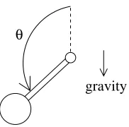
Figure 1: A single-link pendulum.

tasks are either to swing the pendulum’s end point above some height (swing-up) or to swing the pendulum up and balance it in a vertical position (swing-up and balance). In either task, the goal states have greater total mechanical energy than the initial state, which is typically the hanging-down, rest position. Thus, any controller that solves one of these tasks must somehow impart a certain amount of energy to the system. We first demonstrate our approach on a deterministic pendulum swing-up and balance task.

4.1 Problem Definition and Controllers

Figure 1 depicts the pendulum. The state of the pendulum is specified by an angular position,

θ, which is measured counter-clockwise from upright, and an angular velocity, ˙θ. The angular acceleration of the pendulum obeys the dynamics equation

¨

θ=sinθ+u,

where the sine term is due to gravity and u is a control torque. This equation assumes the pendulum is of length one, mass one, and gravity is of unit strength. Since the pendulum’s dynamics are identi-cal at the states(θ+2kπ,θ˙), for k∈ {0,±1,±2,...}, we assume thatθstays in the range[−π,π]. In our simulations, ifθleaves that range, our code returns it to that range by adding or subtracting 2π, as appropriate. We also artificially restricted ˙θto the range[−6,6]. This was important only for the worst-behaved, naive reinforcement learning agents, which sometimes developed control policies that tended to drive the pendulum’s velocity to+∞or−∞.

The particular problem we study is mimimum-time control to a goal set comprising near-upright, near-stationary states: G1 ={(θ,θ˙):k(θ,θ˙)k2 ≤0.01}. We assume that the control torque is bounded in absolute value by umax=0.225. With this torque limit, the pendulum cannot be di-rectly driven to G1. Instead, the solution involves swinging the pendulum back and forth repeatedly, pumping energy into it until there is enough energy to swing upright.

Most reinforcement learning algorithms are designed for discrete-time control. To bridge the gap between the learning algorithms and the continuous-time dynamics of the pendulum, we define a number of continuous-time control laws for the pendulum. Each control law chooses a control torque based on the state of the pendulum. The discrete-time actions of the agents in our experiments correspond to committing control of the pendulum to a specific control law for a specific period of time. Discrete-time control of continuous-time systems is often done in this manner (see Huber and Grupen, 1998b; Branicky et al., 2000, for other examples). In all, we introduce five control laws for the pendulum. The first two are simple constant-torque control laws.

A third control law we use is a saturating linear-quadratic regulator design for the linear approx-imation of the pendulum dynamics centered at the origin. (See Vincent and Grantham, 1997, for details.) For a region of state space surrounding the origin, this controller is sufficient to pull the pendulum into the origin and hold it there.

P3(θ,θ˙) =max(min(−2.4142θ−2.1974 ˙θ,umax),−umax).

In other words, P3 is the function −2.4142θ−2.1972 ˙θ clipped so as to remain in the range

[−umax,+umax]. The constants 2.4142 and 2.1972 come from numerical solution of a matrix equa-tion that is part of the LQR design process; they have no special meaning by themselves.

None of these control laws rely on Lyapunov analysis, and none alone can bring the pendulum to an upright, balanced state from all initial states. We now develop two controllers based on a Lyapunov analysis of the pendulum.

The mechanical energy of the pendulum is ME(θ,θ˙) =1+cos(θ) +1₂θ˙2. The first two terms correspond to gravitational potential energy, and the last term corresponds to kinetic energy. At the origin, the mechanical energy of the pendulum is precisely 2. For any other state with ME=2, if

u is taken to be zero, the pendulum will naturally swing up and asymptotically approach the origin.

So, the pendulum swing-up and balance problem can be reduced to the problem of achieving any state with a mechanical energy of 2.

The time derivative of the pendulum’s mechanical energy is ˙ME(θ,θ˙) =−sin(θ)θ˙+θ˙θ¨=θ˙u. So

a natural control law for rapidly increasing the pendulum’s energy is to choose u to be of magnitude

umax and with sign matching ˙θ. It turns out that this control law has potential difficulties near positions where the control torque of±umax is at equilibrium with the effects of gravity (Perkins, 2002). However, a modification of this rule can avoid the equilibrium point problem. We call this strategy MEA for “modified energy ascent.” Parameterized by w, this rule supplies a control torque of magnitude w in the direction of ˙θ“most of the time.” When that choice is close to equilibrium with gravity, however, the control law switches down to a torque of magnitude w/2, which is not near equilibrium with gravity. The precise formulation is

MEA(w,θ,θ˙) =               

sgn(θ˙)w if|θ˙|>ε˙

or(0<θ˙ <ε˙ andθ∈/E1) or(−˙ε<θ˙ <0 andθ∈/E2) 1

2sgn(θ˙)w if(0<θ˙<ε˙andθ∈E1) or(−˙ε<θ˙ <0 andθ∈E2) sgn(θ)w if ˙θ=0 ,

where sgn(x) ={+1 if x≥0 and−1 if x<0}, ˙ε>0 is a constant (we use ˙ε=0.1 in our ex-periments), and E1 and E2 are sets of states surrounding the equilibrium points of ±w torque

with gravity. In particular, letting θw =sin−1(w) and ε= 1₂(sin−1(w)−sin−1(1₂w)), then E1=

[−π+θw−ε,−π+θw+ε)∪[−θw−ε,−θw+ε)and E2= (θw−ε,θw+ε]∪(π−θw−ε,π−θw+ε]. We use MEA to define two final control laws.

P4(θ,θ˙) =MEA(umax,θ,θ˙),

Experiment Control laws Goal set Summary

1 P4,P5 G2 Descent on L certain.

2 P1,P2,P4,P5 G2 Descent on L possible, not guaranteed. 3 P1,P2 G2 No guarantees.

4 P1,P2,P3 G1 No guarantees.

Figure 2: Control laws and goal sets for Experiments 1–4.

Theorem 3 If the pendulum is controlled continuously by P4or P5 from any initial state, then the

mechanical energy of the pendulum increases monotonically and without bound. Further, from any initial state, if the pendulum is controlled by either P4 or P5 for a period of timeδ, then the

mechanical energy of the pendulum increases by at least some amount∆. The amount∆differs for P4and P5and depends onδ, but it does not depend on the initial state of the pendulum.

Proof sketch: A full proof was presented by Perkins (2002). We sketch the main idea here, focusing on the second claim, from which the first claim follows easily. Recall that ME˙ =θ˙u.

Because P4and P5apply at least 1₄umaxtorque in the direction of ˙θ, we know that the change in ME over a period ofδtime is at least 1₄umax

R_δ

t=0|θ˙(t)|dt,where ˙θ(t)denotes the angular velocity of the pendulum at time t. Since ˙θ(t)can be zero, it is not immediately obvious that the integral should be bounded above zero. Conceivably, ˙θ(t)could stay arbitrarily close to zero, and the integral could be arbitrarily small. Besides keeping ME nonnegative, a key property of MEA is that it keeps ¨˙ θ bounded away from zero, regardless of the state of the pendulum. Thus, MEA ensures that if ˙θ is near zero at some point, it will quickly move away from zero; either the pendulum accelerates rapidly, or it slows rapidly to a stop and accelerates the other way. Thus, ˙θcannot stay near zero for the wholeδtime period, and the integral can be bounded above zero across all possible initial states.

The pendulum can be brought to the upright balanced position by using either P4 or P5 to in-crease the pendulum’s energy to precisely 2, and then letting u=0 so that the pendulum swings up and asymptotically approaches the origin. Is this an optimal strategy? It is not. As we see in the next section, a reinforcement learning controller that learns to switch between P4 and P5 can produce significantly faster swing-up. Allowing switching between other controllers enables even faster swing-up. That P4is significantly suboptimal may be surprising. P4applies magnitude umax torque most of the time, and thus more or less maximizes the instantaneous rate at which energy is pumped into the system. Reasons for its suboptimality, and an explanation of how the learning agents do better, are provided in Section 4.3.

4.2 Experiments

We performed four learning experiments in the deterministic pendulum domain. In each experiment, the agent had different actions to choose from—that is, different sets of control laws with which it could control the pendulum—as summarized in Figure 2. Choosing an action meant that the pendulum was controlled according to the corresponding control law for a period of one second, or until the pendulum entered the goal set.

2, fixing u=0 results in a trajectory which asymptotically approaches the origin and thus enters G1. For these experiments, we defined a surrogate goal set, G2={(θ,θ˙): ME(θ,θ˙) =2}. The cost of a non-terminal action (one that did not bring the pendulum into G2) was one. The cost of a terminal action was equal to the time from the start of the action until the pendulum reached G2, plus the time it took the pendulum to swing up to G1from there. With this cost function, an optimal policy reflects minimum time control to the set G1, even though we used the goal set G2. For Experiment 4, action costs were simply equal to the duration of the action—one for non-terminal actions, and one or less for actions which caused the pendulum to enter G1.

We used the Sarsa(λ) algorithm withλ=0.8 to learn control policies. The action value func-tions were represented using separate CMAC function approximators for each action. Each CMAC covered the range of states−π≤θ≤π and −6≤θ˙ ≤6. Each CMAC had 10 layers, and each layer divided each dimension into 24 bins, for a total of 576 tiles per layer. Offsets were random. The learning rate for the kth_{update of a tile’s weight was 1/}√_{k. (See Sutton and Barto, 1998, for} details and references on Sarsa and CMACs.) We performed 25 independent runs of 20,000 learn-ing trials. Agents chose actions accordlearn-ing to theε-greedy strategy, with ε=0.1. That is, on each time step, with probability 0.1 an agent took an action selected uniformly randomly. Otherwise, the agent chose an action with best estimated action value. Ties were broken randomly. After each learning trial we performed a test trial, in which there was no learning and no exploration, in order to evaluate the current policy. All trials started from state (θ,θ˙) = (π,0). Trials were terminated if they exceeded 900 time steps, which is approximately 50 times longer than the time required to reach G1.

The pendulum dynamics were simulated using 4th-order Runge-Kutta integration with a fixed time step of 0.01 seconds. Because of the fixed time-step size, exactly hitting the G2 goal set in simulation is very unlikely; slightly overshooting ME=2 is the norm. To make our simulation behave more like our theoretical model, we set the pendulum torque to u=−100sgn(θ˙)(ME(θ,θ˙)− 2)instead of u=0 once ME(θ,θ˙)reached or exceeded 2. This shed any slight excess energy the pendulum had, usually on the order of 0.0001, and ensured that the pendulum reached G1correctly. In the first experiment, the agent had two actions to choose from, corresponding to control laws

P4 and P5. By Theorem 3, on any time step, both of the actions for the agent in Experiment 1 either cause the pendulum to enter G2 or increase the mechanical energy by at least some amount

∆>0. Using this fact, we were able to establish a number of qualitative performance guarantees for the agent in Experiment 1. Defining L(θ,θ˙) =2−ME(θ,θ˙) and letting T =G2, we see that the conditions of Theorem 1 are satisfied. This means that the agent was guaranteed to bring the pendulum to G2, and by extension, to G1on every trial (Property 2 with T =G1). If we imagine the pendulum continuing to evolve under u=0 after reaching G1, we know that it would stay in G1 forever and asymptotically approach the origin (Property 3 with T =G1and Property 5 with T =

{(0,0)}). Further, the pendulum was guaranteed to remain in the set T ={(θ,θ˙): ME(θ,θ˙)≤2} at all times, which can be viewed as a safety constraint. The agent could not pump an arbitrarily large amount of energy into the pendulum, which in reality might result in damage to the equipment or dangerously fast motions. In short, we were able to establish many reassuring performance guarantees for the agent by virtue of the actions we designed for it.

not intersect G2. Thus, during test trials, there was no guarantee that the agent would bring the pendulum to the goal. During learning trials, reaching the goal was guaranteed. Recall that during learning trials agents chose a random action on each time step with probability 0.1. This was done to ensure that the agents tried out and learned about all actions. For the agent of Experiment 2, it also ensured some probability of choosing P4or P5on each time step. Since L(θ,θ˙) =2−ME(θ,θ˙) is bounded above on the set {(θ,θ˙): ME(θ,θ˙)<2}, Theorem 2 applies with q=0.1 and p=1. The agent in Experiment 2, then, was guaranteed to bring the pendulum to G1 on every learning trial with probability 1, as long as the trials lasted long enough. (Because trials were limited to 900 seconds, it was possible in principle that the pendulum would not reach the goal in some learning trials. In the next section, however, we observe that no learning trials in Experiment 2 were even one-tenth that long.) The other guarantees established for Experiment 1, that energy stays bounded, and that the pendulum converges to the origin after reaching G2, apply in Experiment 2 as well.

In Experiment 3, there were just two actions, corresponding to control laws P1and P2. By virtue of using the G2goal set, the pendulum was guaranteed to remain in the set T ={(θ,θ˙): ME(θ,θ˙)≤ 2}(Property 1). And the pendulum was guaranteed to approach the origin after reaching G2. But there was no guarantee, during learning or test trials, that the pendulum would reach G2, regardless of the length of those trials.

In Experiment 4, the agent had three actions to choose from, corresponding to control laws P1,

P2, and P3. In this case, we used G1 as the goal set. Initially, we experimented with an agent that chose between just the P1 and P2 control laws. However, it turned out to be extremely difficult to bring the pendulum to the small G1 goal set by switching between+umax and −umaxtorque in discrete time. We added the P3control law in Experiment 4 to make the problem tractable.

We have described the experiments in this order because it represents decreasing dependence on Lyapunov domain knowledge. In Experiment 1, the agent was constrained to make the pendulum ascend on mechanical energy and reach the G2 goal set. In Experiment 2, the agent had actions based on the Lyapunov-designed controllers P4 and P5, and used goal set G2. But the agent was not constrained to increase the pendulum’s mechanical energy at all times. In Experiment 3, we dropped the actions based on the Lyapunov-designed control laws, and in Experiment 4 we dropped the G2goal set. Experiment 4 might be considered the formulation of the control problem that uses the least prior knowledge while still allowing a solution to be learned with reasonable effort.

4.3 Results and Discussion

Figure 3 displays learning curves for the agents in Experiments 1 through 4, plotted on the same scale to facilitate comparison. The dark lines represent the time to G1 during test trials, averaged across the 25 independent runs. The lighter lines represent the shortest and longest test trials across runs. For readability purposes, the curves are smoothed by averaging blocks of 5 trials together; the mean-time-to-goal curve omits trials that time out without reaching G1. The horizontal axis shows the trial number, going up to 1,000 of the 20,000 total trials. By way of comparison, the strategy of using P4to pump energy into the pendulum until it reaches G2and then letting it swing to G1takes 24.83 seconds.

Experiment 1 Experiment 2

200 400 600 800 1000

15 20 25 30 35 40 45 50

trial number

time to goal (min,mean,max)

200 400 600 800 1000

15 20 25 30 35 40 45 50

trial number

time to goal (min,mean,max)

Experiment 3 Experiment 4

200 400 600 800 1000

15 20 25 30 35 40 45 50

trial number

time to goal (min,mean,max)

200 400 600 800 1000

15 20 25 30 35 40 45 50

trial number

time to goal (min,mean,max)

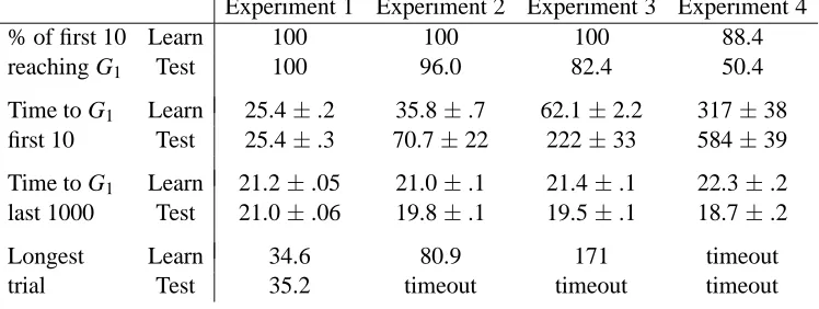
Experiment 1 Experiment 2 Experiment 3 Experiment 4 % of first 10 Learn 100 100 100 88.4 reaching G1 Test 100 96.0 82.4 50.4

Time to G1 Learn 25.4±.2 35.8±.7 62.1±2.2 317±38 first 10 Test 25.4±.3 70.7±22 222±33 584±39

Time to G1 Learn 21.2±.05 21.0±.1 21.4±.1 22.3±.2 last 1000 Test 21.0±.06 19.8±.1 19.5±.1 18.7±.2

Longest Learn 34.6 80.9 171 timeout

trial Test 35.2 timeout timeout timeout

Figure 4: Summary statistics for Experiments 1–4.

are so short in Experiment 1, that agent also learns significantly faster (in terms of total time steps) than the agents in the other experiments. Figure 4 gives more detailed statistics summarizing the experiments. The table reports the percentage of the first ten trials which make it to G1before timing out at 900 time steps, the mean duration of the first ten learning and test trials, the mean duration of the last 1000 learning and test trials, and the longest trials observed in each experiment. The means are accompanied by 95% confidence intervals.

The initial performance of the agent in Experiment 1 was clearly the best, an order of magnitude better than that of the agent in Experiment 4, which incorporated the least prior knowledge. Impor-tantly, only in Experiment 1, for which the strongest theoretical guarantees were established, did the agent bring the pendulum to the goal on every learning and test trial. The longest trial generated in that experiment was 35.2 seconds, whereas all the other experiments included much worse learning trials and test trials that timed out. In this domain, ensuring descent on the Lyapunov function, and not the mere presence of Lyapunov-based actions, is necessary for ensuring good performance at all times.

The performance figures for the final 1000 trials reveal significant improvements from initial performance in all experiments. In the end, all the learning agents also outperform the simple strat-egy of using P4. However, the numbers reveal a down-side to using Lyapunov domain knowledge. The constraint to descend on the Lyapunov function limits the ability of the agent in Experiment 1 to minimize the time to G1. In the final test trials, it takes an average of 21.0 seconds to swing the pendulum upright. The agents in Experiments 2 and 3 do better because they are not constrained in this way. Their final test trials take 19.8 and 19.5 seconds on average. Why is this? Recall that the time derivative of the pendulum’s mechanical energy is ˙ME(θ,θ˙) =θ˙u. In Experiment 1, the

not constrained to choose u=0 once the pendulum had reached G2 and before it had reached G1. The agent was able to continue accelerating the pendulum towards upright and then decelerate it as it approached, resulting in even faster trajectories to G1.

5. Stochastic Pendulum Swing-Up and Balance

In this section, we consider a swing-up and balance problem for a pendulum with stochastic dynam-ics. We formulate the problem as a continuing task, not a goal-based task. The agent seeks to swing the pendulum upright and maintain it upright for as much of the time as possible. The pendulum’s position variable is subject to random disturbances which tend to push the pendulum away from the balanced state, making the task more challenging.

5.1 Dynamics and Controllers

We model the pendulum’s dynamics by the system of stochastic control differential equations:

dθ=θ˙dt+0.1dW ,

d ˙θ=sin(θ)dt+udt ,

where W denotes a Wiener process with mean zero and standard deviation one (see, for example, Kushner, 1971). The Wiener process is the standard model of a continuous-time Gaussian dis-turbance, or “white noise.” The equations above describe a Gaussian disturbance to the position variable, with mean zero and standard deviation 0.1.

As mentioned above, there are no goal states for this problem. The agent’s task is to keep the pendulum near upright as much as possible, where “near upright” is defined by the set Sup=

{(θ,_θ˙_{):|θ| ≤0.5}. The agent incurs unit cost per time as long as the pendulum is not in Sup, and} incurs no cost while the pendulum is in Sup. Sup contains all states up to approximately 30 degrees away from upright.

Because of the random disturbances to the position variable, no controller can maintain the pendulum in the set Sup indefinitely. Indeed, because the disturbance toθis Gaussian, with infinite tails, there is some probability that the pendulum will “jump” out of Sup on any given time step, regardless of how it is controlled. On the other hand, the same disturbances insure that, regardless of how the pendulum is controlled, with probability one it will eventually enter Sup from any initial state. Thus, under any controller the pendulum reaches Sup with probability one (Property 2) and spends an infinite amount of total time there (Property 4). In Section 5.3, however, we will see that these guarantees are very weak, and that controllers that are explicitly designed to return the pendulum to Sup can have a much stronger influence.

We define four new control laws for this problem. One is just the zero torque control law.

P6(θ,θ˙) =0 .

Experiment Control laws Summary

5 P7,P8,P9 Designed to return to Sup; choice of±umaxand 0 in Sup. 6 P1,P2,P6 Choice of±umaxand 0 torques.

Figure 5: Design of Experiments 5 and 6.

swinging upright, passing through Sup quickly, and swinging down again on the other side. In this case, the control laws apply a braking torque to the pendulum, with strength proportional to the amount of excess energy the pendulum has. Intuitively, when the pendulum is outside Sup, these control laws “aim for” the upright, stationary position in the center of Sup. Letting B(θ,θ˙) = max(min(−100sgn(θ˙)(ME(θ,θ˙)−2),umax),−umax) be the braking force applied to a pendulum with energy in excess of 2, we define

P7(θ,θ˙) =

  

+umax if(θ,θ˙)∈Sup

P4(θ,θ˙) if(θ,θ˙)∈/Sup and ME(θ,θ˙)<2

B(θ,θ˙) if(θ,θ˙)∈/Sup and ME(θ,θ˙)≥2 ,

P8(θ,θ˙) =

  

0 if(θ,θ˙)∈Sup

P4(θ,θ˙) if(θ,θ˙)∈/Sup and ME(θ,θ˙)<2

B(θ,θ˙) if(θ,θ˙)∈/Sup and ME(θ,θ˙)≥2 ,

P9(θ,θ˙) =

  

−umax if(θ,θ˙)∈Sup

P4(θ,θ˙) if(θ,θ˙)∈/Sup and ME(θ,θ˙)<2

B(θ,θ˙) if(θ,θ˙)∈/Sup and ME(θ,θ˙)≥2 .

5.2 Experiments

Figure 5 summarizes the two experiments we performed in the stochastic pendulum domain. In Experiment 5, the agent chose from actions corresponding to P7, P8, and P9. This agent did not need to learn how to get the pendulum into Sup. Outside of Sup, all three of its control laws are identical and are designed to do that task. All that the agent had to learn was how best to keep the pendulum in Sup once it was there, by switching among −umax, 0, and+umaxtorques. In Experiment 6, the agent chose from control laws P1, P2, and P6, corresponding to torques−umax, 0, and+umax. This agent had to learn how to get the pendulum into Sup, as well as how to keep it there. Neither agent could keep the pendulum in Sup indefinitely and, for either agent, the pendulum was guaranteed to return to Sup regardless of the choices the agent made. However, the Lyapunov-based actions in Experiment 5 strongly biased that agent toward bringing the pendulum to Sup. At the least, superior initial performance was expected in Experiment 5.

Experiment 5 Experiment 6

100 200 300 400 500

0 200 400 600 800 1000

trial number

time not upright (min,mean,max)

100 200 300 400 500

0 200 400 600 800 1000

trial number

time not upright (min,mean,max)

Figure 6: Mean, min, and max across runs of time spent not near upright during test trials.

Experiment 5 Experiment 6 Cost of first Learn 523±11 848±9 trial Test 468±44 922±28

Mean cost in Learn 366±8 841±4 first 10 trials Test 287±10 925±8

Mean cost in Learn 279±5 301±9 last 100 trials Test 193±7 203±11

Highest cost Learn 555 964

trials Test 635 999

Figure 7: Summary statistics for Experiments 5 and 6.

The pendulum dynamics were simulated using a time step size of 0.1 second. On each time step, 4th-order Runge-Kutta integration was used to compute the deterministic dynamics, after which a mean zero, standard deviation 0.1√0.1 Gaussian disturbance was added to the position variable.

5.3 Results and Discussion

Figure 6 displays learning curves representing the minimum, mean, and maximum test trial costs across the 25 runs. Note that trial cost is the same as time the pendulum spends outside of Sup. These curves are not smoothed, and are plotted for the first 500 of the 1,000 total test trials. By way of comparison, the single best-performing control law for the task is P8, which keeps the pendulum in Sup approximately 43% of the time, corresponding to an average trial cost of around 570.

Figure 7 presents detailed statistics supporting these observations. The difference in perfor-mance between the first trial and first ten trials of Experiment 5 indicates how much learning hap-pened early on. Of course, trials were 999 seconds long, almost 4,000 decision steps, so it is not surprising that significant learning could take place in the first few trials. The performance figures for the final 100 test trials indicate that the agent in Experiment 5 did better than the agent in Ex-periment 6. However, the difference is on the edge of statistical significance. Although the shapes of the learning curves suggest that the agents had reached an asymptotic level of performance, it is possible that with further learning or tweaking of learning parameters, greater performance could be obtained. At any rate, the restriction in Experiment 5 to push the pendulum’s energy towards 2 whenever it is not in Sup appears not to have negatively impacted the agent’s performance. The figures for the highest-cost trials demonstrate once again the benefits of Lyapunov-based designs in ensuring good performance. Even in the worst test trial in Experiment 5, the pendulum was in

Sup for more than one third of the 999 seconds. In the worst learning trial, the pendulum was near

upright for almost half of the time. Experiment 6 included many test trials in which the pendulum spent no time in Sup and some learning trials that were almost as bad.

6. Robot Arm Movement and Stabilization

Robot arm, or manipulator, control is possible through the well-known technique of “feedback linearization,” described below. Feedback linearization is an important tool in control theory and widely used in control practice as well. For robot arm control and other problems, however, control based on feedback linearization is notorious for being inefficient, slow, and “robotic”, and/or for exerting unnecessarily high torques. Feedback linearization does not take advantage of the natural dynamics of the arm. Indeed, the main idea is to use control torque to eliminate most of the natural dynamics, making analytical solution of the problem possible. From an optimal control point of view, then, robot arm control remains an interesting and unsolved problem.

The last two problems we consider are simulated robot arm control problems. We treat the two largely simultaneously, as the only difference between them is that in one case the arm’s dynamics are deterministic and in the other case the dynamics are stochastic. The same goal set, cost function, and sets of control laws are used for both versions of the dynamics.

6.1 Dynamics and Controllers

The robot arm is depicted in Figure 8. Its state is specified by three angular joint positions and three angular velocities. We use x to denote the state vector. The vector of joint positions and the vector of joint velocities are denoted byΘand ˙Θrespectively. For the deterministic version of the dynamics, we use a standard frictionless model (Craig, 1989):

d dt

Θ

˙

Θ

=

_˙

Θ

H−1(Θ,Θ˙)(τ−V(Θ,Θ˙)−

G

,

θ

θ

θ

3 2

1

link length mass

1 2 3

1.0 1.0 1.0

1.0 1.0 1.0

Figure 8: Diagram of the 3-link arm.

multiplicative in the joint velocities.2

d

Θ

˙

Θ

=

_˙

Θ(dt+0.2dW)

H−1(Θ,Θ˙)(τ−V(Θ,Θ˙)−

G

.

Here, W should be interpreted as a vector of three independent Wiener processes with mean zero and standard deviation one. We assume joint positions are limited to the range[−π,+π]. If the dynamics try to push a joint’s position out of this range, its position is held at the edge of the range (that is, at

+πor−π) and the joint’s velocity is set to zero. We do not explicitly bound joint velocities. The task is to move the arm to the goal set Garm={x :kxk ≤0.01}.This is a set of low-velocity states near to a fully-extended horizontal configuration,Θ=0. Rather than having a single initial state, we use an initial state distribution that is uniform over the configurations Θ0= (a,b,−b)for

a∈ {−π,−2₃π,−1₃π}and b∈ {−1₂π,0,+1₂π}, with zero velocity.

As in Experiments 1 through 4, agents’ actions correspond to choosing control laws to apply to the arm for a period of one second. Lettingτ(t), t∈[0,1], denote the torques chosen by a control law during one second of control, and lettingΘ(t) denote the joint positions the arm goes through during that time, we define the cost of choosing that control law to beR₀1kΘ(t)k2+kτ(t)−τ0k2dt, whereτ0is the amount of torque needed to hold the arm steady at the origin. Intuitively, this cost function penalizes the agent to the extent that the state is far from Garmand to the extent that large control torques, beyond the unavoidableτ0, are applied to the arm.

In pilot experiments, we found that it was virtually impossible for an agent to bring the arm to Garm using naive action formulations. With three joints to actuate and a range of torques that need to be applied to reach Garm, a sufficient set of constant-torque actions would be unmanageably large. We also found that a control law based on a linear approximation to the arm dynamics at the origin brought the arm into Garmfor only a fairly small set of surrounding states. It is possible that learning algorithms explicitly designed to handle continuous action spaces could be successful on

the problem (for example, Gullapalli, 1992). However, we used the same approach that we found successful on the pendulum—defining a small set of well-chosen control laws with which an agent can learn to control the arm.

The standard method for controlling a robot arm is to combine feedback linearization with some form of linear system control (Craig, 1989). A simple approach to feedback linearization in the robot arm case is to reparameterize the control torque in terms of a vector u so thatτ=Hu+V+

G

d dt

Θ

˙

Θ

=

_˙

Θ

u

,

for the deterministic case, and

d

_Θ

˙

Θ

=

_Θ˙

(dt+0.2dW)

udt

,

for the stochastic case. Since H is always non-singular, this transformation is lossless; anyτcan be achieved by the proper choice of u. Once the dynamics are expressed in linear form, linear control design methods apply. We use a linear-quadratic regulation (LQR) approach. This results in controllers that are able to move the arm to any desired configuration, and also provides the Lyapunov function which constrains one of the action sets we define below. We briefly describe the LQR approach. (See, for example, Vincent and Grantham, 1997, for a more thorough discussion.)

Consider a linear system of the form ˙x=Ax+Bu, where x is a state vector, u is a control vector,

and A and B are constant matrices. Suppose we want to move this system to a target state xT from any initial state x0, and suppose we specify a control law for performing this task. Let x(t) be a system trajectory that results from that control law. The “quadratic” part of LQR says that the quality of that control law should be measured by the cost function R₀∞[(x(t)−xT)0Q(x(t)−xT) +

u(x(t))0Ru(x(t))]dt, where Q and R are symmetric positive-definite matrices of our choosing. That

is, a quadratic penalty is associated with the deviation of the state, x(t), from the target state, xT, and a quadratic penalty is associated with the control effort u. If we restrict ourselves to control laws of the form u=−K(x−xT), where K is a constant “gain” matrix, then the optimal K can be found by solving a matrix algebraic Ricatti equation. This equation is typically solved numerically, though in the present case it can readily be solved by hand (Perkins, 2002). By varying our choices of Q and

R, we can produce K’s that represent different tradeoffs between the speed of approaching xT and the size of the control effort, u, that is applied.

Note that the cost function of our optimal control problem and the cost function of the LQR design are similar in form. Both include a quadratic penalty on the deviation of the state from the target and a quadratic penalty on control effort. A key difference is that the LQR design penalizes

our reinforcement learning agents are able to discover policies for controlling the arm that use less real effort and/or less time than a standard LQR design.

We define five controllers based on the feedback linearization transformation and LQR design. That is, each controller chooses τ=Hu+V +

G

let Q0be the matrix with diagonal{1,1,1,0.01,0.01,0.01}; let R0be the 3×3 identity matrix; let

K=LQR(Q0,R0); and letΘ4, and Θ5 respectively be the joint position vectors[−1₂π,1₂π,−π], and

[−1

2π,− 1

2π,π]. Our first five control laws for the arm are

A1(Θ,Θ˙) =−H(Θ,Θ˙)K

Θ

˙

Θ

V(Θ,Θ˙) +

G

A2(Θ,Θ˙) =−H(Θ,Θ˙)K2

_Θ

˙

Θ

V(Θ,Θ˙) +

G

A3(Θ,Θ˙) =−H(Θ,Θ˙)K3

Θ

˙

Θ

V(Θ,Θ˙) +

G

A4(Θ,Θ˙) =−H(Θ,Θ˙)K

Θ−Θ4 ˙

Θ

V(Θ,Θ˙) +

G

A5(Θ,Θ˙) =−H(Θ,Θ˙)K

Θ−Θ5 ˙

Θ

V(Θ,Θ˙) +

G

The intuitions behind these control laws are as follows. The first three control laws move the arm to the origin, which is in the center of the goal set, Garm. They move the arm there at different rates, however. Q0 primarily penalizes the arm’s position for being far from the zero position, putting relatively little weight on the arm’s velocity being different from zero. This reflects the fact that we want the arm to be moved to the goal position, but we are not particularly concerned about the velocity of the arm as it goes to the goal. R0puts a unit penalty on control effort, u, so the A1design represents an equal balance between getting the arm to the zero position and exerting control effort.

A2uses a higher penalty on the distance to the goal position; this control law tends to move the arm to the origin more quickly than A1by using a larger control effort, u. A3 is biased in the opposite direction. The final two control laws, A4and A5, do not move the arm into Garmat all. They move it to the configurationsΘ4andΘ5respectively, which are 90 degrees from Garmwith the outer two links of the arm folded in. This can be useful because when the arm is folded, its moment of inertia around the first joint is reduced, allowing it to be swung around that joint with little actual torque.

it is bounded below zero outside of Garm. Thus from any initial state, during any one second period,

A1causes the arm to either enter Garmor descend on Larmby an amount at least∆.

Control laws A2 through A5 do not always cause descent on Larm, but we can readily define similar controllers that do. Let C be any control law. We can define an Larm-descending version as

LD(C,Θ,Θ˙) =

C(Θ,Θ˙) if Larm(Θ,Θ˙)≥0.1 and C(Θ,Θ˙)causes _dtdLarm(Θ,Θ˙)≤ −0.1

A1(Θ,Θ˙) otherwise.

We define four more control laws for the arm as the Larm-descending versions of control laws A2 through A5.

A6(Θ,Θ˙)=LD(A2,Θ,Θ˙) ,

A7(Θ,Θ˙)=LD(A3,Θ,Θ˙) ,

A8(Θ,Θ˙)=LD(A4,Θ,Θ˙) ,

A9(Θ,Θ˙)=LD(A5,Θ,Θ˙) .

Theorem 4 For the deterministic arm dynamics, there exists∆>0 such that for any s∈/Garm, if

the arm is controlled for one second by A1,A6,A7,A8, or A9, then either the arm enters Garmor

the resulting state is at least∆lower on Larm. For the stochastic arm dynamics, there exists∆>0

and p>0 such that for any s∈/Garm, if the arm is controlled for one second by A1,A6,A7,A8, or

A9, then with probability at least p either the arm enters Garm or the resulting state is at least ∆

lower on Larm. For either set of dynamics, in any trajectory created by switching among any of the

controllers A1,...,A9, the system state stays bounded at all times.

Proof sketch: First, we argue boundedness. The Θ component of the state is bounded at all times in the region[−π,π]3. The only concern, then, is with the velocity component of the state,

˙

Θ. All of the control laws above are LQR controllers or combinations of LQR controllers for the feedback-linearized arm. Each LQR controller has feedback gains on the joint velocities which tend to slow each joint down. That is, the acceleration of joint i follows the rule: ¨Θ(i) =−a(Θ(i)−

ΘT(i))−b ˙Θ(i), where a and b are positive constants andΘT(i) is the ith component of the target configuration for the LQR controller. Since Θis bounded, for velocities larger in magnitude than some

V

V

k_Θ˙_0k∞>

_V

_V

Experiment Dynamics Control laws Summary

7 deterministic A1,A6,A7,A8,A9 Descent on Larmguaranteed. 8 deterministic A1,A2,A3,A4,A5 Descent possible, not guaranteed. 9 stochastic A1,A6,A7,A8,A9 Probabilistic descent on Larm. 10 stochastic A1,A2,A3,A4,A5 Descent possible, not guaranteed.

Figure 9: Design of Experiments 7 through 10.

6.2 Experiments

We performed four experiments in the robot arm domain, as outlined in Figure 9. Experiments 7 and 8 used the deterministic version of the dynamics, while Experiments 9 and 10 used the stochastic version. In Experiments 7 and 9, the agent chose from five actions, corresponding to the control laws A1,A6,A7,A8, and A9. In Experiments 8 and 10, the agent chose from actions corresponding to the control laws A1,A2,A3,A4, and A5.

For each experiment, we ran 25 independent runs of Sarsa(λ) withλ=0.8. Each run consisted of 1,000 blocks, or suites, of 18 trials—one learning trial from each of the states in our initial state distribution, followed by one test trial from each initial state. Action selection was ε-greedy with

ε=0.1. Action value functions were represented using a separate CMAC function approximator for each action. Each CMAC covered the region of state space: [−π,π]3×[−5,5]3. Each CMAC had 20 layers, dividing each dimension into 5 equal-sized bins, with offsets being random. The learning rate for the kth _{update of a tile’s weight was 1/}√_{k. Trials were terminated after 250 time steps if} they did not reach Garm.

The deterministic arm dynamics were simulated using 4th-order Runge-Kutta integration with a fixed time step size of 0.1 seconds. The stochastic dynamics were simulated by computing the de-terministic dynamics and then multiplying the change to each joint position by one plus a Gaussian random disturbance with mean zero and standard deviation 0.2√0.1.

By Theorem 4, the formulation of Experiment 7 satisfies the conditions of Theorem 1 with

T =Garm. Thus, that agent was guaranteed to control the arm to Garmon every trial (Property 2). If we assume that, once the arm enters Garm, it continues to be controlled according to A1, then the arm remains in Garmand asymptotically approaches the origin (Properties 3 and 5). Since we know that all of the controllers available in Experiment 7 descend on Larm, a trajectory that starts at state x0is guaranteed not to leave the region{x : L(x)≤L(x0)}(Property 1), which can be viewed as a safety property. For Experiment 9, Theorem 4 implies that the conditions of Theorem 2 are satisfied, thus this agent had a probability one guarantee of controlling the arm to Garmon every trial. Under the stochastic dynamics, no control law can guarantee keeping the arm in Garm. However, one can show using arguments based on martingale theory that A1, for example, has some chance of keeping the arm in Garmforever. This is possible because the position disturbance, which is multiplicative in ˙Θ, vanishes as ˙Θ→0. We do not delve into these arguments here, but see, for example, the book by Kushner (1971).

Experiment 7 Experiment 8

50 100 150 200

250 300 350 400 450 500 550 600 650

test suite number

cost to goal (min,mean,max)

50 100 150 200

250 300 350 400 450 500 550 600 650

test suite number

cost to goal (min,mean,max)

Experiment 9 Experiment 10

50 100 150 200

250 300 350 400 450 500 550 600 650

test suite number

cost to goal (min,mean,max)

50 100 150 200

250 300 350 400 450 500 550 600 650

test suite number

cost to goal (min,mean,max)

Figure 10: Mean, min, and max test suite costs across runs.

or with some probability). Thus, from Theorems 2 and 4, these agents were guaranteed to bring the arm to Garmduring learning trials, if given enough time.

6.3 Results and Discussion

Learning curves for the four experiments are displayed in Figure 10. We define the cost of a test suite (a set of nine test trials, one from each initial state) to be the average of the costs of the nine trials. The curves plot the minimum, mean, and maximum test suite costs, across runs, for the first 200 of 1,000 test suites. Using control law A1 alone generates a test suite cost of 434 under the deterministic dynamics and 448, on average, under the stochastic dynamics.

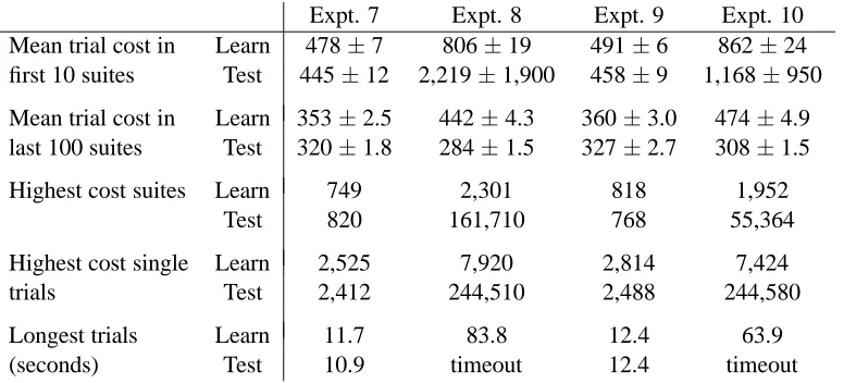
Expt. 7 Expt. 8 Expt. 9 Expt. 10 Mean trial cost in Learn 478±7 806±19 491±6 862±24 first 10 suites Test 445±12 2,219±1,900 458±9 1,168±950

Mean trial cost in Learn 353±2.5 442±4.3 360±3.0 474±4.9 last 100 suites Test 320±1.8 284±1.5 327±2.7 308±1.5

Highest cost suites Learn 749 2,301 818 1,952 Test 820 161,710 768 55,364

Highest cost single Learn 2,525 7,920 2,814 7,424 trials Test 2,412 244,510 2,488 244,580

Longest trials Learn 11.7 83.8 12.4 63.9 (seconds) Test 10.9 timeout 12.4 timeout

Figure 11: Summary statistics for Experiments 7–10.

shows that the position disturbance in the stochastic dynamics has essentially no qualitative effect on learning. Its primary effect is to make performance during learning and test trials more noisy.

Summary statistics are presented in Figure 11. For the most part, these statistics support what is visible in the learning curves—better initial performance and lower variability performance for the agents with a Lyapunov-descent constraint, but better final performance for the unconstrained agents. One thing not readily observed from the learning curves is the powerful effect Lyapunov-descent constraints have on worst-case behavior. In the worst test suites and the worst individual test trials, agents without Lyapunov constraints incurred two orders of magnitude more cost than the constrained agents. There was a similar disparity in the durations of the longest trials for the two types of agents. As in the other experiments above, Experiments 7–10 demonstrate that constrain-ing an agent to descend on a Lyapunov function is important in ensurconstrain-ing reasonable performance. Merely providing actions that are designed using Lyapunov analysis does not ensure good behavior.

7. Related Work

The methods for safe agent design that we propose in this paper rely on qualitative analysis ideas that have been under development for more than a century. Lyapunov originally developed the idea of a Lyapunov function late in the 19th_{century. The idea that there is more than one way for a system} to descend on a given Lyapunov function, and that this freedom can be used to optimize secondary criteria, dates back at least to Kalman and Bertram’s early survey of Lyapunov function methods (1960). Subsequent work has used this observation in various ways, sometimes to optimize a cost function as we do here, and sometimes to produce controllers with improved stability or robustness properties. (See, for example, Krsti´c et al., 1995; Freeman and Kokotovi´c, 1996; and Sepulchre et al., 1997, for work of this sort and further references.) Viewed in this light, the primary novelty of our work is the application of these ideas to learning systems, in which we are concerned with on-line learning behavior and cannot necessarily trust the behavior of a learned policy.