2017; 6(4-1): 72-82
http://www.sciencepublishinggroup.com/j/acm doi: 10.11648/j.acm.s.2017060401.17
ISSN: 2328-5605 (Print); ISSN: 2328-5613 (Online)
Global Optimization with Descending Region Algorithm
Loc Nguyen
Vietnam Institute of Mathematics, Hanoi, Vietnam
Email address:
To cite this article:
Loc Nguyen. Global Optimization with Descending Region Algorithm. Applied and Computational Mathematics. Special Issue: Some Novel Algorithms for Global Optimization and Relevant Subjects. Vol. 6, No. 4-1, 2017, pp. 72-82. doi: 10.11648/j.acm.s.2017060401.17
Received: April 8, 2017; Accepted: April 10, 2017; Published: June 9, 2017
Abstract:
Global optimization is necessary in some cases when we want to achieve the best solution or we require a new solution which is better the old one. However global optimization is a hazard problem. Gradient descent method is a well-known technique to find out local optimizer whereas approximation solution approach aims to simplify how to solve the global optimization problem. In order to find out the global optimizer in the most practical way, I propose a so-called descending region (DR) algorithm which is combination of gradient descent method and approximation solution approach. The ideology of DR algorithm is that given a known local minimizer, the better minimizer is searched only in a so-called descending region under such local minimizer. Descending region is begun by a so-called descending point which is the main subject of DR algorithm. Descending point, in turn, is solution of intersection equation (A). Finally, I prove and provide a simpler linear equation system (B) which is derived from (A). So (B) is the most important result of this research because (A) is solved by solving (B) many enough times. In other words, DR algorithm is refined many times so as to produce such (B) for searching for the global optimizer. I propose a so-called simulated Newton – Raphson (SNR) algorithm which is a simulation of Newton – Raphson method to solve (B). The starting point is very important for SNR algorithm to converge. Therefore, I also propose a so-called RTP algorithm, which is refined and probabilistic process, in order to partition solution space and generate random testing points, which aims to estimate the starting point of SNR algorithm. In general, I combine three algorithms such as DR, SNR, and RTP to solve the hazard problem of global optimization. Although the approach is division and conquest methodology in which global optimization is split into local optimization, solving equation, and partitioning, the solution is synthesis in which DR is backbone to connect itself with SNR and RTP.Keywords:
Global Optimization, Gradient Descent Method, Descending Region, Descending Point1. Introduction
The local optimization problem is specified simply as follows [1]:
min
subject to = 0, ∀ = 1, !≤ 0, ∀ = 1,
Where f called target function is analytic and convex. All constraints ui and vj are convex functions. The Lagrangian
function is composed as follows [2, p. 215]:
" , #, $ = + & #
'
()
+ & $
*
()
Where,
# = #), #+, … , #'
-$ = -$), $+, … , $*
-Variables λ and µ are called Lagrange multipliers [3]. Note that the notation T denotes transposition operator because λ
and µ are column vectors. As default, vectors mentioned in this research are column vectors if there is no additional explanation. If there is no constraint, Lagrangian function is the target function f. The duality principle is derived from local optimization problem as follows [4, p. 160]:
.
∗= argmin " , #, $
#∗, $∗ = argmax
The point x* is called local optimizer or local minimum
point, which is also the saddle point of Lagrangian function. If
x* is a local optimizer, it satisfies Karush – Kuhn – Tucke (KKT) condition [5] as follows:
8 9 : 9
;∂" , #, $∂ = 0
= ≤ 0, ℎ = 0, ∀ = 1, , ∀ = 1, ! $ ≥ 0, ∀ = 1,
$ = = 0, ∀ = 1,
Where @A ,4,5@ is partial derivative of L(x, λ, µ) with regard to x. In practice, x* is solved by combination of duality principle and KKT condition. Concretely, suppose a triple (x*,
λ*, µ*) is solution of following equation system:
8 9 : 9
;∂" , #, $∂ = 0 ∂" , #, $
∂# = B- and ∂" , #, $∂$ = B
-$ = 0 and ∗ = 0, ∀ = 1, , ∀ = 1, !
Where 0 denotes zero vector 0 = (0, 0,…, 0)T whereas
@A ,4,5 @4 and
@A ,4,5
@5 are partial derivatives of L(x, λ, µ) with
regard to λ and µ, respectively, which are row vectors as follows:
∂" , #, $
∂# = D∂" , #, $∂#) ,
∂" , #, $ ∂#+ , … ,
∂" , #, $ ∂#' E
∂" , #, $
∂$ = D∂" , #, $∂$) ,
∂" , #, $ ∂$+ , … ,
∂" , #, $ ∂$* E
If such triple (x*, λ*, µ*) satisfies following condition, x* is a local optimizer:
F$∗≥ 0, ∀ = 1,∗ ≤ 0, ∀ = 1,
Alternately, gradient descent (GD) method [6] is also used to find out x* with regard to f. This research is inspired from GD method.
The global optimization is general form of local optimization as follows [7, p. 109]:
minG | ∈ JK
Where f is arbitrary and J = L | ≤ 0, =
0, ∀ = 1, , ∀ = 1, !M is arbitrary set.
A point x* is called global optimizer or global minimum point if f(x*) ≤ f(x) for all x belonging S. Because the cost of finding out x* is very expensive, the approximation solution
approach issues a concept of global ε-optimization with
acceptance of small error ε [7, p. 135]. The global optimizer x*
is replaced by a so-called global ε-optimizer ̅ as follows [7, p. 123]:
≥ ̅ − P, ∀ ∈ J
Let z0 be an arbitrary point and set k=0, the approximation
solution approach has two phases to find out QR as follows [7, p. 124]:
1.From zk, searching for xk as a local optimizer.
2.If xk is proved as the global ε-minimizer then, return
̅ = S. Otherwise, find out a feasible solution z such
that f(z) < f(xk) and then, set k=k+1, set zk=z, and go back phase 1.
As a convention, superscript numbers (in z0, zk, xk, etc.) denote indices if there is no additional explanation. This research focuses on global optimization, in which I propose a so-called descending region (DR) algorithm that is a practical implementation of approximation solution approach. I use the very small value ε as a downward shift to determine the feasible point z in phase 2 and I use GD method to search for local optimizer. As a result, the final point is the global ε-minimizer. In other words, DR algorithm is simpler and it is an advanced variant of GD method. Section 2 is full description of DR algorithm which has two steps for each iteration, corresponding with two phases of theoretical approximation solution. The feasible point z is called descending point. It is possible to consider DR algorithm to be combination of GD method and approximation solution approach, which aims to solve global optimization problem in practical way. GD method follows descending direction which is the opposite of gradient to reach local optimizer. Note that gradient is the first derivative of multivariate function. GD is described in subsection 2.1. There are some alternatives of GD method such as particle swarm optimization (PSO) and Quasi-Newton method.
PSO [8] was firstly invented by James Kennedy and Russell Eberhart in 1995 and later on, it attracts many researchers. PSO is inspired from bird flocking, fish schooling, and swarming theory [8, p. 1942] in which a swarm of individuals (birds, fishes, etc.) called particles moves in the searching space in order to reach the global optimizer. Each particle owns a position and a velocity. The movement of each particle, which is change of its position and velocity, is affected by itself and other particles (swarm) [9]. The swarm’s position is the best one over all particles’ positions. At the ith iteration, the swarm’s position xi is best if it satisfies most fitness criterion [10, p. 3]; as usual, f(xi) is as small as possible. After a finite number of movements, the swarm’s position reaches to global optimizer. The meaning of velocity is approximate to the meaning of gradient but velocity is not gradient. So PSO does not require target function f to be analytic [9]. Quasi-Newton method [11] is an alternative of Newton’s method to find out local optimizer in case that Hessian matrix, which is second derivative of multivariable function, is not existent or not easy to be computed. Quasi-Newton method finds out a solution of the equation created by setting gradient to be zero [11], as local optimizer. Quasi-Newton method updates Hessian matrix by successive gradients after iterations [11].
algorithm partitions domain space into sub-rectangles and lower bound of each sub-rectangle is calculated based on solution of LRP. The final lower bound is the minimum one over all sub-rectangles. If deviation between upper bound and lower bound is smaller than ε, the global ε-optimal solution of relaxation problem is determined. The convergence of branch and bound algorithm is proved [12, pp. 193-194]. Larsson and Patriksson [13] allowed duality gap to be nonzero in order to find out the near-optimizer which is an approximation of global optimizer with concepts of ε-optimality and δ-complementarity [13, p. 439]. They establish the new condition of global optimality with duality gap size ε + δ to solve the near-optimizer [13, p. 441]. The literature of global optimization and relevant subject is very large. Please read the book “Convex Analysis
and Global Optimization” of Tuy Hoang [7] to comprehend
theory of global optimization. This research only focuses on practical implementation of ε-optimality approach. Section 2 is full description of DR algorithm. Section 3 describes how to solve intersection equation by simulated Newton – Raphson (SNR) algorithm in order to find out descending region necessary to DR algorithm. In turn, section 4 describes how to determine the starting point necessary to SNR algorithm, by random testing point (RTP) algorithm. Section 5 is the conclusion with some suggestions in future trend. In general, the global optimization problem is divided into three smaller problems such as local optimization, solving equation, and partitioning which are solved by three algorithms such as DR, SNR, and RTP, respectively. DR algorithm is the most important one, which is connect itself with SNR and RTP.
2. Descending Region Algorithm
Suppose f is the target analytic function that we need to find out its global optimizer with regard that f is scalar-by-vector function (multivariate function).
: U → ℝ
Where ℝ is real number field and U is real vector space such that U ⊆ ℝ*. Suppose f is arbitrary but U is convex. Descending region (DR) algorithm is iterative algorithm whose input is an initial point ω0 and the output is global optimizer z**. The ideology of DR algorithm is that given a known local optimizer z*, the better local optimizer is searched only in a so-called descending region under the known point z*. If the target function has global minimum value, DR algorithm is terminated after a finite number of iterations; at that time the local optimizer z* approaches the global optimizer z**. In DR algorithm, the descending region is begun by a so-called
descending point which is defined as the point under the
optimizer z* and so the next better optimizer is searched under descending point. Suppose zi is the descending point at the ith
iteration and zi is initialized by ω0. DR algorithm has many iterations and each iteration includes two steps:
1.Step 1: Searching for local optimizer step.
2.Step 2: Determining descending region step.
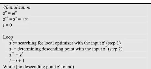
Such two steps are implementations of two phases of approximation solution approach [7, p. 124]. In general, Table 1 shows the pseudo-code like for DR algorithm. Note, the input is an arbitrary point ω0 and the output is global optimizer z**.
Table 1. DR algorithm.
//Initialization
z0 = ω0
z** = z* = +∞
i = 0
Loop
z*:= searching for local optimizer with the input zi (step 1)
zi:= determining descending point with the input z* (step 2)
z** = z*
i = i + 1
While (no descending point zi found)
2.1. Searching for Local Optimizer Step
With the descending point zi, I apply GD method [1] [6] to find out the local optimizer z*. Note that zi is initialized by ω0. We know that GD method is also iterative method; suppose at the iteration jthin this method, the next candidate point YZ) is computed as follows [6]:
YZ)= Y + [ \
Where,
- The point Y is the previous candidate point and Y is initialized by the starting point zi.
- The direction \ is the descending direction, which is the opposite of gradient of function f. We have \ =
−∇ ^Y _ where ∇ denotes the gradient of function f. - The value [ is the length of the descending direction
\.
After m iterations, the point Y converges to the local optimizer z*. If the terminated condition of GD method is equal to 0 ^\ = B-_ then, z* is likely local optimizer and we go to step 2. Otherwise, the terminated condition is that GD method runs after m iterations, we compare the current optimizer z* with the previous optimizer y*:
- If z* is equal to y*, then DR algorithm stops and z* is the global optimizer, z** = z*.
- If z* is not equal to y*, then go to step 2.
2.2. Determining Descending Region Step
Given the local optimizer z* found out in step 1 and let ε be a very small pre-defined positive number, ε >0. The number ε
is also called descending error. Let h(x) be hyper-plane that goes through the level f(z*)– ε and is parallel to the abscissa hyper-plane or domain plane of function f, we have:
ℎ Q = Y∗ − P
Let f* = f(z*) be the minimum value of target function f at z*, we have:
ℎ Q = ∗− P
The intersection between hyper-plane h(x) and the function
f(x) is a contour at level f* – ε with note that f(x) is a hyper-surface. Following is the equation of such contour:
Or,
Q − ∗+ P = 0
Note that this equation is called intersection equation. If the contour is not existent; in other words, if the hyper-plane h(x) does not intersect with the surface f(x), then DR algorithm is stopped and z* is the global optimizer and we have z** = z*. Otherwise, suppose z0 is a point that belongs to the contour; in other words, z0 is a solution of the equation f(x) = f* – ε with note that the method to find out z0 is proposed later, then we do two important tasks:
- Increasing i by 1, we have i = i+1.
- The new descending point zi is assigned by the solution
z0 and we have zi = z0 with attention that the index i was increased by 1. After that, we go back step 1.
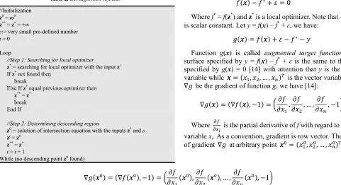
It is easy to recognize that the next better local optimizer is searched only in the region under the solution z0. This region is descending region. So this algorithm is called descending region (DR) algorithm and solution z0 is also called descending point. Although both zi and z0 are called descending points, the point zi is known as descending point at the ith iteration and z0 is solution of the equation f(x) = f* – ε. In Table 2, the pseudo-code for DR algorithm is refined with note that the input is an arbitrary point ω0 and the output is global optimizer z**.
Table 2. DR algorithm refined.
//Initialization
z0 = ω0
z** = z* = +∞
ε:= very small pre-defined number
i = 0
Loop
//Step 1: Searching for local optimizer
z*:= searching for local optimizer with the input zi If z* not found then
break
Else If z* equal previous optimizer then
z** = z* break End If
//Step 2: Determining descending region
z0:= solution of intersection equation with the inputs z* and ε
zi = z0
z** = z*
i = i + 1
While (no descending point z0 found)
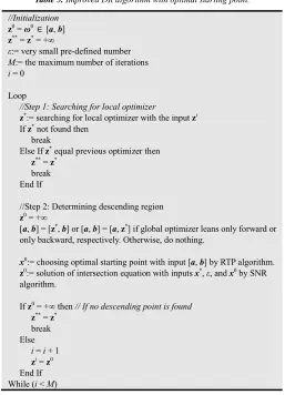
For example, given target one-variable function
=161 b− 1
12 d−34 +−23
Given initial point ω0 = (–2.76, –1), it is easy to receive the first local optimizer x* = (–2, –2) by applying gradient method. Suppose the very small number ε is 1, the descending point z0
which is solution of intersection equation f(x) – f* + ε = f(x) – (– 2) + 1 = f(x) + 3 = 0 is solved by the method mentioned in next section; hence we get z0 = (1.84, –3). Starting from z0 = (1.84, – 3), the next local optimizer is found out, x* = (3, –4.6) by applying gradient method again. The new intersection equation
f(x) + 5.6 = 0 has no solution and it is concluded that the global optimizer is x** = (3, –4.6). Fig. 1 depicts this example.
3. Method to Determine Descending
Region
As aforementioned, descending pointz0 is a solution of the equation of the intersection between hyper-plane h(x) and target function f(x) and descending region is the region under the solution z0. So determining descending region is equivalent to solving the intersection equation specified by (1) in order to find out its solution z0.
Q − ∗+ P = 0 (1)
Where f* = f(z*) and z* is a local optimizer. Note that – f* + ε
is scalar constant. Let y = f(x) – f* + ε, we have:
= Q = Q + P − ∗− g
Function g(x) is called augmented target function. The surface specified by y = f(x) – f* + ε is the same to the one specified by g(x) = 0 [14] with attention that y is the scalar variable while Q = ), +, … , * - is the vector variable. Let
∇= be the gradient of function g, we have [14]:
∇= Q = ∇ Q , −1 = hii
),
i i +, … ,
i i *, −1j
Where kkl
m is the partial derivative of f with regard to partial
variable xi. As a convention, gradient is row vector. The value
of gradient ∇= at arbitrary point Q7= )7, +7, … , *7 - is:
∇= Q7 = ∇ Q7 , −1 = hi
i ) Q 7 ,i
i + Q 7 , … ,i
i * Q 7 , −1j
Where kkl
n Q
7 is the value of partial derivative of f with regard to partial variable x
i of x0. Please distinguish the arbitrary
starting point x0 from the initial point ω0 of DR algorithm mentioned in previous section. The gradient ∇= is normal vector of tangent hyper-plane of g and so this tangent hyper-plane at point x0 is specified by following equation [14]:
∇= Q7 h Q − Q7
g − Q7 + ∗− Pj = 0 ⇔ hii ) Q
7 ,i
i + Q 7 , … , i
i * Q
7 , −1j ∗ h Q − Q7
g − Q7 + ∗− Pj = 0
)− )7 ii ) Q
7 + +− +7 i
i + Q
7 + ⋯ + *− *7 i
i * Q
7 − g − Q7 + ∗− P = 0
So we have:
g = Q7 − ∗+ P + & − 7 i
i
*
()
Q7
It implies
g = ∇ Q7 Q + Q7 − ∗+ P − ∇ Q7 Q7
Equation (2) is the hyper-line which represents the intersection between tangent hyper-plane and the hyper-plane y = 0 and so it is called intersection hyper-line.
∇ Q7 Q − p7= 0 (2)
Where c0 is a scalar value:
p7= ∇ Q7 Q7+ ∗− Q7 − P
Equation (2) has many solutions which are points belonging to it. Now we find out only one solution x1 of (2) with regard that
x1 satisfies two following conditions:
1.Point x1 is the projection of x0 on the intersection hyper-line. 2.Point x1 belongs to intersection hyper-line.
The first condition implies that the vector p1 = x0 – x1 is parallel to orthogonal vector of intersection hyper-line. It is easy to infer from (2) that such orthogonal vector is ∇ Q7 . Therefore, the first condition is interpreted by following equation:
q)= r∇ Q7 ⇔
8 99 : 99
; )7− ))= rii ) Q
7
+7− +)= rii + Q
7
⋮
*7− *)= rii
* Q
7
⇔
8 99 : 99
; ))+ 0 + ⋯ + 0 + rii
) Q
7 =
)7
0 + +)+ ⋯ + 0 + rii + Q
7 = +7
⋮ 0 + 0 + ⋯ + *)+ rii
* Q
7 = *7
Where Q)= )), +), … , *) - and l are unknowns. The second condition implies that x1 satisfies (2).
∇ Q7 Q)− p7= 0 ⇔ ))ii
) Q
7 +
+)ii + Q
7 + ⋯ + *)ii
* Q
7 = p7
We set up the set of equations so as to determine x1 as below:
8 9 9 9 : 9 9 9
; ))+ 0 + ⋯ + 0 + rii ) Q
7 =
)7
0 + +)+ ⋯ + 0 + rii
+ Q
7 =
+7
⋮
0 + 0 + ⋯ + *)+ rii
* Q
7 =
*7
))ii
) Q
7 +
+)ii
+ Q
7 + ⋯ + *)ii
* Q
7 + 0 = p7
t7= u v v v v v v
w 1 0 ⋯ 0
i i ) Q
7
0 1 ⋯ 0 ii
+ Q 7
⋮ ⋮ ⋱ ⋮ ⋮
0 0 ⋯ 1 ii
* Q
7
i i ) Q
7 i
i + Q
7 ⋯ i
i * Q
7 0 y z z z z z z {
|7= DQ7
p7E =
u v w )7 +7 ⋮ *7
p7y
z {
p7= ∇ Q7 Q7+ ∗− Q7 − P
The projection system is re-written, as seen in (3):
t7}Q)
r ~ = |7 (3)
Matrix A0 is called projection matrix and vector b0 is called projection vector. The determinant of matrix A0 denoted |A0|is not equal to 0 if and only ifthe gradient ∇ Q7 is not equal to 0T. Suppose |A0| is not equal to 0, it is easy to find out x1 by Cramer’s method as follows [15, pp. 136-138]:
Q)= • )) +)
⋮
*)
€ =|t17| • |t)7|
|t+7|
⋮ |t*7|
€
Let t7 is the matrix constructed by replacing jth column in matrix A0 by projection vector b0.
I proposed the iterative method which is a simulation of the Newton – Raphson method [16, pp. 67-71] so as to solve (1) based on (3). The proposed method is called simulated Newton
– Raphson (SNR) algorithm. Suppose we have an
approximate solution xk at the kth iteration, we set up the projection system based on xk in order to find out the next better solution xk+1; hence xk+1 is solution of (4).
tShQSZ)
r j = |S (4)
Where,
tS=
u v v v v v v
w 1 0 ⋯ 0
i i ) Q
S
0 1 ⋯ 0 ii
+ Q S
⋮ ⋮ ⋯ ⋮ ⋮
0 0 ⋯ 1 ii
* Q
S
i i ) Q
S i
i + Q
S ⋯ i
i * Q
S 0 y z z z z z z {
|S = DQS
pSE =
u v w )S +S ⋮ *S
pSy
z {
pS= ∇ QS QS+ ∗− QS − P
As aforementioned, the positive number ε is a very small pre-defined number and f* is the local minimum value at z*. Note that Ak and bk are totally determined according to xk and
xk is initialized by an arbitrary point x0. It is easy to infer that the solution xk+1 is calculated as below:
QSZ)=
u w
)SZ) +SZ)
⋮
*SZ)y
{ = 1|tS| u v w•t)
S•
•t+S•
⋮ |t*S|y
z {
Where tS is the matrix constructed by replacing jth column in projection matrix Ak by projection vectorbk.
It is easy to recognize that xk+1 is calculated based on previous xk and so SNR algorithm is an iterative process. If the descending pointz0 which is solution of (1) is existent then, xk
will approach z0 after a finite number of iterations. In other words, the descending region which supports us to search for global optimizer is determined.
The convergence of SNR algorithm is dependent on the starting point x0. If x0 is not in the volume where SNR algorithm converges, no solution z0 is found although there is existence of solutions of (1). Moreover, the closer to descending point z0 the point x0 is, the faster the convergence speed is. So the way to choose right x0 is very important, which is mentioned in next section.
There are two terminated conditions of SNR algorithm to determine descending point z0:
- Equation (1) has a solution xk where f(xk) is equal or approximated to 0 at the kth iteration, f(xk) ≈ 0. At that time we have z0 = xk.
- Equation (1) has no solution when the determinant |Ak| is equal to 0 at the kth iteration.
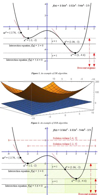
It is necessary to make a simple example of SNR algorithm. Suppose f*=1, ε=1, and f(x) is approximated to x12 + x22 – 4 in
solution volume where the superscript number “2” denotes the square. Some advanced methods such as feasible length [17] and minimizing square error [18] are suggested to approximate f by Taylor polynomial. The augmented target function is g(x) = x12 +
x22 + ε – f* – y = x12 + x22 – 4 – y. The gradient of f is ∇ Q =
2 ), 2 + . Given starting point x0 = (2, 1)T, at the first iteration, we have the initial solution as follows:
Q7 = 1
t7= ‚1 0 20 1 0
2 0 0ƒ
|7= 2,1,9
-The SNR algorithm converges at the 4th iteration with x4 = (1.79, 0.89)T and f(x4) ≈ 0. So we have the descending point z0
= x4 = (1.79, 0.89)T. In Fig. 2, the target surface f is marked yellow and the tangent hyper-plane of f at x4 (y = –8 + 3.58x1 +
1.79y) is marked blue.
Because the cost of solving (1) by SNR algorithm is significant, it is necessary to test whether (1) has solution or not before finding out the descending point. If there is no existence of solutions of (1), DR algorithm is stopped and we concludes that the current local optimizer z* is global optimizer z**. In practice, we often apply DR algorithm into finding out the global optimizer in a given volume [a, b] which is an interval in ℝ, rectangle in ℝ+ or volume in ℝd.
Therefore, if (1) is a polynomial equation, p(x) = 0 where
p(x) = f(x) – (f(z*) + ε) is a polynomial and x is scalar unknown, there is some methods to determine interval of solutions, for example, given p(x) = anxn + an-1xn-1 +…+ a1x1 + a0 and let A
be the largest among absolute values of coefficients, A = max
{|a1|, |a2|,…, |an-1|, |an|}, then the upper bound u of all real
solutions is calculated as below [6]:
= 1 +ˆ‡
*
Where an is the coefficient of xn with attention that the
number n denotes the nth power when we often use the superscript number to denote index. If u is smaller than lower bound a of given interval [a, b], then (1) has no solution. We can use another method, Sturm’s theorem [6] [19], to determine the number of distinct real solutions located in given interval [a, b]. If (1) is arbitrary equation, we still use the terminated condition |Ak| = 0 and so how to choose optimal starting point x0 is very important and is mentioned in next section.
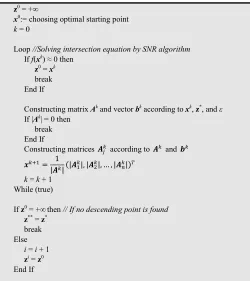
There is a case that target function f has infinitely many local optimizers, which means that f has no global optimizer. This case leads DR algorithm to run in infinite loop. So we add one more terminated condition that DR algorithm will stop after M iterations. In Table 3, the pseudo-code for DR algorithm is refined again with note that the input is an arbitrary point ω0 and the output is global optimizer z**.
Table 3. Final version of DR algorithm.
//Initialization
z0 = ω0
z** = z* = +∞
ε:= very small pre-defined number
M:= the maximum number of iterations
i = 0
Loop
//Step 1: Searching for local optimizer
z*:= searching for local optimizer with the input zi
If z* not found then break
Else If z* equal previous optimizer then
z** = z* break End If
//Step 2: Determining descending region
z0 = +∞
x0:= choosing optimal starting point
k = 0
Loop //Solving intersection equation by SNR algorithm
If f(xk) ≈ 0 then
z0 = xk break End If
Constructing matrix Ak and vector bk according to xk, z*, and ε If |Ak| = 0 then
break End If
Constructing matrices tS according to tS and |S
QSZ)= 1
|tS| |t)S|, |t+S|, … , |t*S| -k = k + 1
While (true)
If z0 = +∞then // If no descending point is found
z** = z*
break Else
i = i + 1
zi = z0
End If
While (i < M) //prevent infinite loop when there is no global maximum
4. Choosing Optimal Starting Point for
Solving Intersection Equation
Given (1), the problem needs solved is to select the starting point x0 so that such point is in the volume where SNR algorithm converges. The volume is defined as the sub-space or sub-set, denoted v(a, b) or [a, b].
‰, | = Š‰, |‹ = Šˆ), Œ)‹ × Šˆ+, Œ+‹ × … × Šˆ*, Œ*‹
The capacity of volume is defined by following formula:
p ‰, | = Ž Œ − ˆ
*
()
Volume can be an interval v(a, b) = [a, b] in ℝ, a rectangle
v(a, b) = [a1, b1] x [a2, b2] in ℝ+ or a volume v(a, b) = [a1, b1]
x [a2, b2] x [a3, b3] in ℝd. Note that the volume is infinite
volume if any of its bound is infinite, for example:
‰, | = Š‰, |‹ = Š−∞, Œ)‹ × Šˆ+, Œ+‹ × … × Šˆ*, +∞‹
If the volume is infinite volume, its capacity is positive infinite, c(a, b) = +∞.
Solution volume is defined as the volume in which solution
of (1) is existent. It is easy to recognize that [a, b] is the solution volume of function f if and only if there exist two values x and y belonging to [a, b] such that f(x)f(y) ≤ 0 according to Bolzano-Cauchy’s theorem [6].
solution volume [a, b] such that [a, b] is as small as possible. In other words, given pre-defined volume [a, b], what we need to do is to find out the sub-volume [ai,bi] so that it satisfies three conditions:
1.It is in [a, b]; in other words, [ai,bi] ⊆ [a, b]. 2.It is also solution volume, satisfying (5).
3.It is as small as possible. This condition helps SNR algorithm to converge as fast as possible.
Such sub-volume is called optimal volume. Because it is impossible to determine optimal volume by calculating exhaustedly f(x) for all x in [ai, bi], I propose a so-called
random testing point (RTP) algorithm to find out optimal
volume. Firstly, suppose x and y are points in [ai,bi] such that
f(x) > 0 and f(y) < 0, respectively. Hence, x and y are called positive point and negative point, respectively. Let ”Z and
”• be the number of positive and negative points, respectively and let pi be the ratio of ”• to the number of total points ” in optimal volume [ai,bi], according to (6).
– = —˜m —™mZ—˜m=
—˜m
—m (6)
Where ” = ”Z+ ”• is the number of total points and so,
pi is the probability of occurrence of negative points in optimal volume [ai,bi]. RTP algorithm to find out optimal volume is based on two heuristic assumptions:
- If [ai,bi] is optimal volume, then the probability 0 < pi < 1, in other words, both ”Z> 0 and ”•> 0.
- The nearer to ½ the probability pi is, the more likely it is that [ai,bi] is optimal volume.
RTP algorithm is iterative algorithm whose input is volume [a, b] and output is optimal volume [ai, bi]. Given volume [a, b] = [a1, b1] x [a2, b2] x … x [an, bn] is divided into n*n
sub-volumes [ai, bi] = [ˆ), Œ)] x [ˆ+, Œ+] x … x [ˆ*, Œ*] where i = 1, . RTP algorithm has finitely many iterations. We do two tasks at each iteration:
1.Creating many enough random points in each volume [ai,
bi].
2.Counting the number of positive and negative points, ”Z and ”• and calculating the probability pi of each sub-volume [ai, bi] based on ”Z and ”•. Which sub-volume that has probability pi being larger than 0 and smaller than 1 and nearest to ½ is chosen to be the input for next iteration.
There are two stopped conditions of RTP algorithm: 1.The deviation between probability pi and ½ or the
capacity c(ai, bi) is smaller than a small pre-defined number δ.
2.Or, the algorithm reaches the maximum number of iterations.
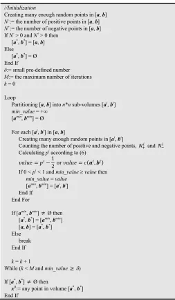
When the optimal volume is determined, the optimal starting point x0 is any point in such volume. Of course, if there is a random point ci ∈ [ai, bi] such that f(ci) = 0, then we have x0 = ci. In general, Table 4 shows the pseudo-code for RTP algorithm whose input is volume [a, b] and output is optimal starting point x0.
Table 4. RTP algorithm to find out optimal starting point.
//Initialization
Creating many enough random points in [a, b]
N–:= the number of positive points in [a, b]
N+:= the number of negative points in [a, b] If N– > 0 and N+ > 0 then
[a*, b*] = [a, b] Else
[a*, b*] = Ø End If
δ:= small pre-defined number
M:= the maximum number of iterations
k = 0
Loop
Partitioning [a, b] into n*n sub-volumes [ai, bi]
min_value = +∞ [amin, bmin] = Ø
For each [ai, bi] in [a, b]
Creating many enough random points in [ai, bi]
Counting the number of positive and negative points, ”Z and ”• Calculating pi according to (6)
ˆr › = – −12 or ˆr › = p ‰ , |
If 0 < pi < 1 and min_value ≥ value then
min_value = value
[amin, bmin] = [ai, bi] End If
End For
If [amin, bmin] ≠ Ø then [a*, b*] = [amin, bmin] [a, b] = [a*, b*] Else
break End If
k = k + 1
While (k < M and min_value≥δ)
If [a*, b*] ≠ Ø then
x0:= any point in volume [a*, b*] End If
The essence of RTP algorithm is to narrow solution volume according to horizontal axis; similarly, the essence of DR algorithm is to narrow the descending region according to vertical axis. If the descending region is also reduced according horizontal axis, DR algorithm will converge faster. Suppose in horizontal axis, DR algorithm begin seeking local optimizers in given initial volume [a, b], such volume is called
searching volume, which is reduced after each iteration. If the
current local optimizer is x* then, the next searching volume is [x*, b] with assumption that the global optimizer leans only forward. In other words, the next descending point z0 is searched in [x*, b] according to horizontal axis and below f(x*) according to vertical axis. Of course, the solution volume of RTP algorithm to find out optimal starting point is [x*, b]. In general, the descending region is reduced according to both horizontal axis and vertical axis. Back the example in section 2.2, given target function,
=161 b− 1
Fig. 3 depicts how to find out global optimizer of target function by the improved DR algorithm. In Fig. 3, two descending regions are shaded areas. It is easy to recognize that the descending areas are narrowed according to two axes. The pseudo-code for DR algorithm is improved as seen in Table 5 with note that the input is an arbitrary point ω0 and searching volume [a, b] and the output is global optimizer z**
with note that [a, b] can be infinite volume.
Table 5. Improved DR algorithm with optimal starting point.
//Initialization
z0 = ω0∈ [a, b]
z** = z* = +∞
ε:= very small pre-defined number
M:= the maximum number of iterations
i = 0
Loop
//Step 1: Searching for local optimizer
z*:= searching for local optimizer with the input zi
If z* not found then break
Else If z* equal previous optimizer then
z** = z* break End If
//Step 2: Determining descending region
z0 = +∞
[a, b] = [z*, b] or [a, b] = [a, z*] if global optimizer leans only forward or only backward, respectively. Otherwise, do nothing.
x0:= choosing optimal starting point with input [a, b] by RTP algorithm.
z0:= solution of intersection equation with inputs x*, ε, and x0 by SNR algorithm.
If z0 = +∞ then // If no descending point is found
z** = z*
break Else
i = i + 1
zi = z0 End If While (i < M)
5. Conclusion
The essence of DR algorithm is to solve the linear system equation (4) many enough times, which aims to solve intersection equation (1). In other words, the hazard problem
of global optimization is turned back the most common problem with note that linear equation system is always solvable. However, that SNR algorithm to solve (1) via (4) is a simulation of Newton – Raphson method causes a new problem of convergence. This is the weak point of the research that I alleviate by RTP algorithm based on partitioning solution space and generating random testing points in order to find out optimal starting point for fast convergence. Currently, I cannot research out a new method better than SNR algorithm. Therefore DR algorithm will be improved significantly if we can predict that (1) has no solution before solving it or we can predict the solution volume of (1). Sturm’s theorem mentioned in section 3 is a good prediction tool but it is only applied into the case that (1) is a polynomial. RTP algorithm with random point generation is also not an optimal tool. However, for my opinion, the prediction approach is potential. In the future, I will research deeply how to approximate (1) into simpler forms such as exponent function and polynomial in order to apply easily prediction tools. For example, (1) can be easily approximated by Taylor polynomial. The smaller the searching volume is, the more accurate the Taylor polynomial is. If the volume is one-dimension interval, optimal degree of Taylor polynomial is equal to or larger than the length of such interval according to [17]. Alternately, Taylor polynomial can be also optimized by minimizing square error according to [18]. I suggest a so-called
segmentation approach in which the solution volume is split
into many small enough segments. Later on, for each segment, approximation methods such as feasible length and minimizing square error are applied to approximate (1) by a Taylor polynomial in such segment so that it is accurate to predict solution volume of such polynomial. Final solution volume of (1) is the best one from many polynomials over all segments. This approach shares the same ideology of volume partitioning with RTP algorithm. It can be more complicated but better than RTP.
Figure 1. An example of DR algorithm.
Figure 2. An example of SNR algorithm.
Acknowledgements
I express my deep gratitude to Professor Le, Dung-Muu and Professor Ta, Duy-Phuong – Vietnam Institute of Mathematics who reviewed and gave me valuable advices to improve this research.
Nomenclature
DR: descending region GD: gradient descent RTP: random testing point
SNR: simulated Newton – Raphson
References
[1] M. D. Le and Y. H. Le, “Lecture Notes on Optimization,” Vietnam Institute of Mathematics, Hanoi, 2014.
[2] S. Boyd and L. Vandenberghe, Convex Optimization, New York, NY: Cambridge University Press, 2009, p. 716.
[3] Y.-B. Jia, “Lagrange Multipliers,” 2013.
[4] A. P. Ruszczyński, Nonlinear Optimization, Princeton, New Jersey: Princeton University Press, 2006, p. 463.
[5] Wikipedia, “Karush–Kuhn–Tucker conditions,” Wikimedia Foundation, 4 August 2014. [Online]. Available:
http://en.wikipedia.org/wiki/Karush–Kuhn–Tucker_conditions. [Accessed 16 November 2014].
[6] P. D. Ta, “Numerical Analysis Lecture Notes,” Vietnam Institute of Mathematics, Hanoi, 2014.
[7] T. Hoang, Convex Analysis and Global Optimization, Dordrecht: Kluwer, 1998, p. 350.
[8] J. Kennedy and R. Eberhart, “Particle Swarm Optimization,” in Proceedings of IEEE International Conference on Neural Networks, 1995.
[9] Wikipedia, “Particle swarm optimization,” Wikimedia Foundation, 7 March 2017. [Online]. Available:
https://en.wikipedia.org/wiki/Particle_swarm_optimization. [Accessed 8 April 2017].
[10] R. Poli, J. Kennedy and T. Blackwell, “Particle swarm optimization,” Swarm Intelligence, vol. 1, no. 1, pp. 33-57, June 2007.
[11] Wikipedia, “Quasi-Newton method,” Wikimedia Foundation, 4 April 2017. [Online]. Available:
https://en.wikipedia.org/wiki/Quasi-Newton_method. [Accessed 8 April 2017].
[12] H. Jiao, Z. Wang and Y. Chen, “Global optimization algorithm for sum of generalized polynomial,” Applied Mathematical Modelling, vol. 37, no. 1-2, pp. 187-197, 18 February 2012. [13] T. Larsson and M. Patriksson, “Global optimality conditions
for discrete and nonconvex optimization - With applications to Lagrangian heuristics and column generation,” Operations Research, vol. 54, no. 3, pp. 436-453, 21 April 2003.
[14] P. Dawkins, “Gradient Vector, Tangent Planes and Normal Lines,” Lamar University, 2003. [Online]. Available:
http://tutorial.math.lamar.edu/Classes/CalcIII/GradientVectorT angentPlane.aspx. [Accessed 2014].
[15] V. H. H. Nguyen, Linear Algebra, Hanoi: Hanoi National University Publishing House, 1999, p. 291.
[16] R. L. Burden and D. J. Faires, Numerical Analysis, 9th Edition ed., M. Julet, Ed., Brooks/Cole Cengage Learning, 2011, p. 872.
[17] L. Nguyen, “Feasible length of Taylor polynomial on given interval and application to find the number of roots of equation,” International Journal of Mathematical Analysis and Applications, vol. 1, no. 5, pp. 80-83, 10 January 2015. [18] L. Nguyen, “Improving analytic function approximation by
minimizing square error of Taylor polynomial,” International Journal of Mathematical Analysis and Applications, vol. 1, no. 4, pp. 63-67, 21 October 2014.
[19] Wikipedia, “Sturm’s theorem,” Wikimedia Foundation, 2014. [Online]. Available: