Hyperband: A Novel Bandit-Based Approach to
Hyperparameter Optimization
Lisha Li [email protected]
Carnegie Mellon University, Pittsburgh, PA 15213
Kevin Jamieson [email protected]
University of Washington, Seattle, WA 98195
Giulia DeSalvo [email protected]
Google Research, New York, NY 10011
Afshin Rostamizadeh [email protected]
Google Research, New York, NY 10011
Ameet Talwalkar [email protected]
Carnegie Mellon University, Pittsburgh, PA 15213 Determined AI
Editor:Nando de Freitas
Abstract
Performance of machine learning algorithms depends critically on identifying a good set of hyperparameters. While recent approaches use Bayesian optimization to adaptively select configurations, we focus on speeding up random search through adaptive resource allocation and early-stopping. We formulate hyperparameter optimization as a pure-exploration non-stochastic infinite-armed bandit problem where a predefined resource like iterations, data samples, or features is allocated to randomly sampled configurations. We introduce a novel algorithm,Hyperband, for this framework and analyze its theoretical properties, providing several desirable guarantees. Furthermore, we compareHyperbandwith popular Bayesian optimization methods on a suite of hyperparameter optimization problems. We observe thatHyperbandcan provide over an order-of-magnitude speedup over our competitor set on a variety of deep-learning and kernel-based learning problems.
Keywords: hyperparameter optimization, model selection, infinite-armed bandits, online optimization, deep learning
1. Introduction
In recent years, machine learning models have exploded in complexity and expressibility at the price of staggering computational costs. Moreover, the growing number of tuning parameters associated with these models are difficult to set by standard optimization techniques. These “hyperparameters” are inputs to a machine learning algorithm that govern how the algorithm’s performance generalizes to new, unseen data; examples of hyperparameters include those that impact model architecture, amount of regularization, and learning rates. The quality of a predictive model critically depends on its hyperparameter configuration, but it is poorly understood how these hyperparameters interact with each other to affect the resulting model.
c
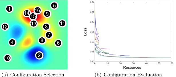
(a) Configuration Selection (b) Configuration Evaluation
Figure 1: (a) The heatmap shows the validation error over a two-dimensional search space with red corresponding to areas with lower validation error. Configuration selection methods adaptively choose new configurations to train, proceeding in a sequential manner as indicated by the numbers. (b) The plot shows the validation error as a function of the resources allocated to each configuration (i.e. each line in the plot). Configuration evaluation methods allocate more resources to promising configurations.
Consequently, practitioners often default to brute-force methods like random search and grid search (Bergstra and Bengio, 2012).
In an effort to develop more efficient search methods, the problem of hyperparameter optimization has recently been dominated by Bayesian optimizationmethods (Snoek et al., 2012; Hutter et al., 2011; Bergstra et al., 2011) that focus on optimizing hyperparameter
configuration selection. These methods aim to identify good configurations more quickly than standard baselines like random search by selecting configurations in an adaptive manner; see Figure 1(a). Existing empirical evidence suggests that these methods outperform random search (Thornton et al., 2013; Eggensperger et al., 2013; Snoek et al., 2015b). However, these methods tackle the fundamentally challenging problem of simultaneously fitting and optimizing a high-dimensional, non-convex function with unknown smoothness, and possibly noisy evaluations.
2017a), we focus on speeding up random search as it offers a simple and theoretically principled launching point (Bergstra and Bengio, 2012).1
We develop a novel configuration evaluation approach by formulating hyperparameter optimization as a pure-exploration adaptive resource allocation problem addressing how to allocate resources among randomly sampled hyperparameter configurations.2 Our procedure,
Hyperband, relies on a principled early-stopping strategy to allocate resources, allowing it
to evaluate orders-of-magnitude more configurations than black-box procedures like Bayesian optimization methods. Hyperband is a general-purpose technique that makes minimal
assumptions unlike prior configuration evaluation approaches (Domhan et al., 2015; Swersky et al., 2014; Gy¨orgy and Kocsis, 2011; Agarwal et al., 2011; Sparks et al., 2015; Jamieson and Talwalkar, 2015).
Our theoretical analysis demonstrates the ability of Hyperbandto adapt to unknown
convergence rates and to the behavior of validation losses as a function of the hyperparameters. In addition,Hyperbandis 5×to 30×faster than popular Bayesian optimization algorithms
on a variety of deep-learning and kernel-based learning problems. A theoretical contribution of this work is the introduction of the pure-exploration, infinite-armed bandit problem in the non-stochastic setting, for which Hyperband is one solution. When Hyperband is
applied to the special-case stochastic setting, we show that the algorithm comes within log factors of known lower bounds in both the infinite (Carpentier and Valko, 2015) and finite
K-armed bandit settings (Kaufmann et al., 2015).
The paper is organized as follows. Section 2 summarizes related work in two areas: (1) hyperparameter optimization, and (2) pure-exploration bandit problems. Section 3 describesHyperband and provides intuition for the algorithm through a detailed example.
In Section 4, we present a wide range of empirical results comparing Hyperband with
state-of-the-art competitors. Section 5 frames the hyperparameter optimization problem as an infinite-armed bandit problem and summarizes the theoretical results for Hyperband.
Finally, Section 6 discusses possible extensions of Hyperband.
2. Related Work
In Section 1, we briefly discussed related work in the hyperparameter optimization literature. Here, we provide a more thorough coverage of the prior work, and also summarize significant related work on bandit problems.
2.1 Hyperparameter Optimization
Bayesian optimization techniques model the conditional probabilityp(y|λ) of a configuration’s performance on an evaluation metricy (i.e., test accuracy), given a set of hyperparametersλ.
1. Random search will asymptotically converge to the optimal configuration, regardless of the smoothness or structure of the function being optimized, by a simple covering argument. While the rate of convergence for random search depends on the smoothness and is exponential in the number of dimensions in the search space, the same is true for Bayesian optimization methods without additional structural assumptions (Kandasamy et al., 2015).
Sequential Model-based Algorithm Configuration (SMAC), Tree-structure Parzen Estimator (TPE), and Spearmint are three well-established methods (Feurer et al., 2014). SMAC uses random forests to model p(y|λ) as a Gaussian distribution (Hutter et al., 2011). TPE is a non-standard Bayesian optimization algorithm based on tree-structured Parzen density estimators (Bergstra et al., 2011). Lastly, Spearmint uses Gaussian processes (GP) to model
p(y|λ) and performs slice sampling over the GP’s hyperparameters (Snoek et al., 2012). Previous work compared the relative performance of these Bayesian searchers (Thornton et al., 2013; Eggensperger et al., 2013; Bergstra et al., 2011; Snoek et al., 2012; Feurer et al., 2014, 2015). An extensive survey of these three methods by Eggensperger et al. (2013) introduced a benchmark library for hyperparameter optimization called HPOlib, which we use for our experiments. Bergstra et al. (2011) and Thornton et al. (2013) showed Bayesian optimization methods empirically outperform random search on a few benchmark tasks. However, for high-dimensional problems, standard Bayesian optimization methods perform similarly to random search (Wang et al., 2013). Recent methods specifically designed for high-dimensional problems assume a lower effective dimension for the problem (Wang et al., 2013) or an additive decomposition for the target function (Kandasamy et al., 2015). However, as can be expected, the performance of these methods is sensitive to required inputs; i.e. the effective dimension (Wang et al., 2013) or the number of additive components (Kandasamy et al., 2015).
Gaussian processes have also been studied in the bandit setting using confidence bound acquisition functions (GP-UCB), with associated sublinear regret bounds (Srinivas et al., 2010; Gr¨unew¨alder et al., 2010). Wang et al. (2016) improved upon GP-UCB by removing the need to tune a parameter that controls exploration and exploitation. Contal et al. (2014) derived a tighter regret bound than that for GP-UCB by using a mutual information
acquisition function. However, van der Vaart and van Zanten (2011) showed that the learning rate of GPs are sensitive to the definition of the prior through an example with a poor prior where the learning rate degraded from polynomial to logarithmic in the number of observations n. Additionally, without structural assumptions on the covariance matrix of the GP, fitting the posterior is O(n3) (Wilson et al., 2015). Hence, Snoek et al. (2015a) and Springenberg et al. (2016) proposed using Bayesian neural networks, which scale linearly with n, to model the posterior.
Adaptive configuration evaluation is not a new idea. Maron and Moore (1997) and Mnih and Audibert (2008) considered a setting where the training time is relatively inexpensive (e.g.,k-nearest-neighbor classification) and evaluation on a large validation set is accelerated by evaluating on an increasing subset of the validation set, stopping early configurations that are performing poorly. Since subsets of the validation set provide unbiased estimates of its expected performance, this is an instance of the stochastic best-arm identification problem for multi-armed bandits (see the work by Jamieson and Nowak, 2014, for a brief survey).
drastically suffer when they are violated. Krueger et al. (2015) proposed a heuristic based on sequential analysis to determine stopping times for training configurations on increasing subsets of the data. However, the theoretical correctness and empirical performance of this method are highly dependent on a user-defined “safety zone.”
Several hybrid methods combining adaptive configuration selection and evaluation have also been introduced (Swersky et al., 2013, 2014; Domhan et al., 2015; Kandasamy et al., 2016; Klein et al., 2017a; Golovin et al., 2017). The algorithm proposed by Swersky et al. (2013) uses a GP to learn correlation between related tasks and requires the subtasks as
input, but efficient subtasks with high informativeness for the target task are unknown without prior knowledge. Similar to the work by Swersky et al. (2013), Klein et al. (2017a) modeled the conditional validation error as a Gaussian process using a kernel that captures the covariance with downsampling rate to allow for adaptive evaluation. Swersky et al. (2014), Domhan et al. (2015), and Klein et al. (2017a) made parametric assumptions on the
convergence of learning curves to perform early-stopping. In contrast, Golovin et al. (2017) devised an early-stopping rule based on predicted performance from a nonparametric GP model with a kernel designed to measure the similarity between performance curves. Finally, Kandasamy et al. (2016) extended GP-UCB to allow for adaptive configuration evaluation by defining subtasks that monotonically improve with more resources.
In another line of work, Sparks et al. (2015) proposed a halving style bandit algorithm that did not require explicit convergence behavior, and Jamieson and Talwalkar (2015) analyzed a similar algorithm originally proposed by Karnin et al. (2013) for a different setting, providing theoretical guarantees and encouraging empirical results. Unfortunately, these halving style algorithms suffer from the “n versus B/n” problem, which we will discuss in Section 3.1. Hyperbandaddresses this issue and provides a robust, theoretically
principled early-stopping algorithm for hyperparameter optimization.
We note thatHyperbandcan be combined with any hyperparameter sampling approach
and does not depend on random sampling; the theoretical results only assume the validation losses of sampled hyperparameter configurations are drawn from some stationary distribution. In fact, subsequent to our submission, Klein et al. (2017b) combined adaptive configuration selection withHyperbandby using a Bayesian neural network to model learning curves and
only selecting configurations with high predicted performance to input intoHyperband.
2.2 Bandit Problems
Pure exploration bandit problems aim to minimize the simple regret, defined as the distance from the optimal solution, as quickly as possible in any given setting. The pure-exploration multi-armed bandit problem has a long history in the stochastic setting (Even-Dar et al., 2006; Bubeck et al., 2009), and was recently extended to the non-stochastic setting by Jamieson and Talwalkar (2015). Relatedly, the stochastic pure-exploration infinite-armed bandit problem was studied by Carpentier and Valko (2015), where a pull of each armiyields an i.i.d. sample in [0,1] with expectation νi, whereνi is a loss drawn from a distribution
with cumulative distribution function,F. Of course, the value ofνi is unknown to the player,
Section 5.3.2. However, their algorithm was derived specifically for the β-parameterization of F, and furthermore, they must estimate β before running the algorithm, limiting the algorithm’s practical applicability. Also, the algorithm assumes stochastic losses from the arms and thus the convergence behavior is known; consequently, it does not apply in our hyperparameter optimization setting.3 Two related lines of work that both make use of an underlying metric space are Gaussian process optimization (Srinivas et al., 2010) andX -armed bandits (Bubeck et al., 2011), or bandits defined over a metric space. However, these works either assume stochastic rewards or need to know something about the underlying function (e.g. an appropriate kernel or level of smoothness).
In contrast, Hyperband is devised for the non-stochastic setting and automatically
adapts to unknown F without making any parametric assumptions. Hence, we believe our work to be a generally applicable pure exploration algorithm for infinite-armed bandits. To the best of our knowledge, this is also the first work to test out such an algorithm on a real application.
3. Hyperband Algorithm
In this section, we present theHyperbandalgorithm. We provide intuition for the algorithm,
highlight the main ideas via a simple example that uses iterations as the adaptively allocated resource, and present a few guidelines on how to deploy Hyperbandin practice.
3.1 Successive Halving
Hyperband extends the SuccessiveHalving algorithm proposed for hyperparameter
optimization by Jamieson and Talwalkar (2015) and calls it as a subroutine. The idea behind the originalSuccessiveHalvingalgorithm follows directly from its name: uniformly
allocate a budget to a set of hyperparameter configurations, evaluate the performance of all configurations, throw out the worst half, and repeat until one configuration remains. The algorithm allocates exponentially more resources to more promising configurations. Unfortunately,SuccessiveHalving requires the number of configurationsnas an input
to the algorithm. Given some finite budget B (e.g., an hour of training time to choose a hyperparameter configuration), B/nresources are allocated on average across the configura-tions. However, for a fixedB, it is not clear a priori whether we should (a) consider many configurations (largen) with a small average training time; or (b) consider a small number of configurations (smalln) with longer average training times.
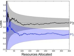
We use a simple example to better understand this tradeoff. Figure 2 shows the validation loss as a function of total resources allocated for two configurations with terminal validation lossesν1 andν2. The shaded areas bound the maximum deviation of the intermediate losses
from the terminal validation loss and will be referred to as “envelope” functions.4 It is possible to distinguish between the two configurations when the envelopes no longer overlap. Simple arithmetic shows that this happens when the width of the envelopes is less than
ν2−ν1, i.e., when the intermediate losses are guaranteed to be less than ν2−2ν1 away from the
3. See the work by Jamieson and Talwalkar (2015) for detailed discussion motivating the non-stochastic setting for hyperparameter optimization.
Figure 2: The validation loss as a function of total resources allocated for two configurations is shown. ν1 andν2 represent the terminal validation losses at convergence. The
shaded areas bound the maximum distance of the intermediate losses from the terminal validation loss and monotonically decrease with the resource.
terminal losses. There are two takeaways from this observation: more resources are needed to differentiate between the two configurations when either (1) the envelope functions are wider or (2) the terminal losses are closer together.
However, in practice, the optimal allocation strategy is unknown because we do not have knowledge of the envelope functions nor the distribution of terminal losses. Hence, if more resources are required before configurations can differentiate themselves in terms of quality (e.g., if an iterative training method converges very slowly for a given data set or if randomly selected hyperparameter configurations perform similarly well), then it would be reasonable to work with a small number of configurations. In contrast, if the quality of a configuration is typically revealed after a small number of resources (e.g., if iterative training methods converge very quickly for a given data set or if randomly selected hyperparameter configurations are of low-quality with high probability), then n is the bottleneck and we should choose nto be large.
Certainly, if meta-data or previous experience suggests that a certain tradeoff is likely to work well in practice, one should exploit that information and allocate the majority of resources to that tradeoff. However, without this supplementary information, practitioners are forced to make this tradeoff, severely hindering the applicability of existing configuration evaluation methods.
3.2 Hyperband
Hyperband, shown in Algorithm 1, addresses this “nversus B/n” problem by considering
several possible values ofnfor a fixed B, in essence performing a grid search over feasible value ofn. Associated with each value of nis a minimum resourcer that is allocated to all configurations before some are discarded; a larger value of ncorresponds to a smaller r and hence more aggressive early-stopping. There are two components toHyperband; (1) the
inner loop invokes SuccessiveHalvingfor fixed values ofn andr (lines 3–9) and (2) the
outer loop iterates over different values of nand r (lines 1–2). We will refer to each such run of SuccessiveHalvingwithinHyperband as a “bracket.” Each bracket is designed
Algorithm 1:Hyperbandalgorithm for hyperparameter optimization. input :R,η (defaultη= 3)
initialization :smax=blogη(R)c,B = (smax+ 1)R
1 for s∈ {smax, smax−1, . . . ,0}do 2 n=dBR η
s
(s+1)e, r=Rη −s
// begin SuccessiveHalving with (n, r) inner loop
3 T =get hyperparameter configuration(n) 4 fori∈ {0, . . . , s} do
5 ni=bnη−ic
6 ri =rηi
7 L={run then return val loss(t, ri) :t∈T}
8 T =top k(T, L,bni/ηc)
9 end
10 end
11 return Configuration with the smallest intermediate loss seen so far.
andB/n. Hence, a single execution of Hyperband takes a finite budget of (smax+ 1)B;
we recommend repeating it indefinitely.
Hyperband requires two inputs (1) R, the maximum amount of resource that can
be allocated to a single configuration, and (2)η, an input that controls the proportion of configurations discarded in each round of SuccessiveHalving. The two inputs dictate how many different brackets are considered; specifically,smax+ 1 different values for nare
considered with smax =blogη(R)c. Hyperband begins with the most aggressive bracket
s=smax, which setsnto maximize exploration, subject to the constraint that at least one
configuration is allocated R resources. Each subsequent bracket reducesn by a factor of approximately η until the final bracket, s= 0, in which every configuration is allocated
R resources (this bracket simply performs classical random search). Hence, Hyperband
performs a geometric search in the average budget per configuration and removes the need to selectnfor a fixed budget at the cost of approximately smax+ 1 times more work than
running SuccessiveHalving for a single value ofn. By doing so, Hyperbandis able to
exploit situations in which adaptive allocation works well, while protecting itself in situations where more conservative allocations are required.
Hyperband requires the following methods to be defined for any given learning problem:
• get hyperparameter configuration(n) – a function that returns a set of n i.i.d. samples from some distribution defined over the hyperparameter configuration space. In this work, we assume uniformly sampling of hyperparameters from a predefined space (i.e., hypercube with min and max bounds for each hyperparameter), which immediately yields consistency guarantees. However, the more aligned the distribution is towards high quality hyperparameters (i.e., a useful prior), the betterHyperband
s= 4 s= 3 s= 2 s= 1 s= 0
i ni ri ni ri ni ri ni ri ni ri
0 81 1 27 3 9 9 6 27 5 81
1 27 3 9 9 3 27 2 81
2 9 9 3 27 1 81
3 3 27 1 81
4 1 81
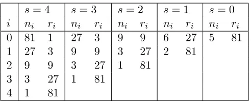
Table 1: The values ofni and ri for the brackets of Hyperband corresponding to various
values of s, whenR= 81 and η = 3.
• run then return val loss(t, r)– a function that takes a hyperparameter configu-rationtand resource allocationr as input and returns the validation loss after training the configuration for the allocated resources.
• top k(configs, losses, k)– a function that takes a set of configurations as well as their associated losses and returns the top kperforming configurations.
3.3 Example Application with Iterations as a Resource: LeNet
We next present a concrete example to provide further intuition about Hyperband. We
work with the MNIST data set and optimize hyperparameters for the LeNet convolutional neural network trained using mini-batch stochastic gradient descent (SGD).5 Our search space includes learning rate, batch size, and number of kernels for the two layers of the network as hyperparameters (details are shown in Table 2 in Appendix A).
We define the resource allocated to each configuration to be number of iterations of SGD, with one unit of resource corresponding to one epoch, i.e., a full pass over the data set. We setR to 81 and use the default value of η= 3, resulting in smax= 4 and thus 5 brackets of SuccessiveHalving with different tradeoffs betweennand B/n. The resources allocated
within each bracket are displayed in Table 1.
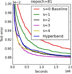
Figure 3 shows an empirical comparison of the average test error across 70 trials of the individual brackets of Hyperband run separately as well as standard Hyperband.
In practice, we do not know a priori which bracket s∈ {0, . . . ,4} will be most effective in identifying good hyperparameters, and in this case neither the most (s= 4) nor least aggressive (s= 0) setting is optimal. However, we note that Hyperband does nearly as
well as the optimal bracket (s= 3) and outperforms the baseline uniform allocation (i.e., random search), which is equivalent to brackets= 0.
3.4 Different Types of Resources
While the previous example focused on iterations as the resource, Hyperbandnaturally generalizes to various types of resources:
Figure 3: Performance of individual bracketssand Hyperband.
• Time– Early-stopping in terms of time can be preferred when various hyperparameter configurations differ in training time and the practitioner’s chief goal is to find a good hyperparameter setting in a fixed wall-clock time. For instance, training time could be used as a resource to quickly terminate straggler jobs in distributed computation environments.
• Data Set Subsampling– Here we consider the setting of a black-box batch training algorithm that takes a data set as input and outputs a model. In this setting, we treat the resource as the size of a random subset of the data set withR corresponding to the full data set size. Subsampling data set sizes using Hyperband, especially for
problems with super-linear training times like kernel methods, can provide substantial speedups.
• Feature Subsampling – Random features or Nystr¨om-like methods are popular methods for approximating kernels for machine learning applications (Rahimi and Recht, 2007). In image processing, especially deep-learning applications, filters are usually sampled randomly, with the number of filters having an impact on the performance. Downsampling the number of features is a common tool used when hand-tuning hyperparameters; Hyperbandcan formalize this heuristic.
3.5 Setting R
The resource R and η (which we address next) are the only required inputs toHyperband.
As mentioned in Section 3.2, R represents the maximum amount of resources that can be allocated to any given configuration. In most cases, there is a natural upper bound on the maximum budget per configuration that is often dictated by the resource type (e.g., training set size for data set downsampling; limitations based on memory constraint for feature downsampling; rule of thumb regarding number of epochs when iteratively training neural networks). If there is a range of possible values forR, a smallerR will give a result faster (since the budget B for each bracket is a multiple ofR), but a larger R will give a better guarantee of successfully differentiating between the configurations.
the budget over time, B ∈ {2,4,8,16, . . .}, and for each B, tries all possible values of
n ∈
2k : k ∈ {1, . . . ,log2(B)} . For each combination of B and n, the algorithm runs an instance of the (infinite horizon)SuccessiveHalving algorithm, which implicitly sets R= 2 logB
2(n), thereby growing R asB increases. The main difference between the infinite
horizon algorithm and Algorithm 1 is that the number of unique brackets grows over time instead of staying constant with each outer loop. We will analyze this version of Hyperband
in more detail in Section 5 and use it as the launching point for the theoretical analysis of standard (finite horizon)Hyperband.
Note thatR is also the number of configurations evaluated in the bracket that performs the most exploration, i.es=smax. In practice one may wantn≤nmax to limit overhead
associated with training many configurations on a small budget, i.e., costs associated with initialization, loading a model, and validation. In this case, set smax = blogη(nmax)c.
Alternatively, one can redefine one unit of resource so that R is artificially smaller (i.e., if the desired maximum iteration is 100k, defining one unit of resource to be 100 iterations will give R= 1,000, whereas defining one unit to be 1k iterations will give R= 100). Thus, one unit of resource can be interpreted as the minimum desired resource andR as the ratio between maximum resource and minimum resource.
3.6 Setting η
The value of η is a knob that can be tuned based on practical user constraints. Larger values ofη correspond to more aggressive elimination schedules and thus fewer rounds of elimination; specifically, each round retains 1/η configurations for a total ofblogη(n)c+ 1 rounds of elimination withn configurations. If one wishes to receive a result faster at the cost of a sub-optimal asymptotic constant, one can increase η to reduce the budget per bracketB = (blogη(R)c+ 1)R. We stress that results are not very sensitive to the choice ofη. If our theoretical bounds are optimized (see Section 5), they suggest choosingη =e≈2.718, but in practice we suggest takingη to be equal to 3 or 4.
Tuningηwill also change the number of brackets and consequently the number of different tradeoffs thatHyperbandtries. Usually, the possible range of brackets is fairly constrained,
since the number of brackets is logarithmic inR; namely, there are (blogη(R)c+ 1) =smax+ 1
brackets. For our experiments in Section 4, we choseη to provide 5 brackets for the specified
R; for most problems, 5 is a reasonable number ofnversusB/ntradeoffs to explore. However, for largeR, usingη = 3 or 4 can give more brackets than desired. The number of brackets can be controlled in a few ways. First, as mentioned in the previous section, if R is too large and overhead is an issue, then one may want to control the overhead by limiting the maximum number of configurations to nmax, thereby also limitingsmax. If overhead is not a
concern and aggressive exploration is desired, one can (1) increase η to reduce the number of brackets while maintaining R as the maximum number of configurations in the most exploratory bracket, or (2) still use η = 3 or 4 but only try brackets that do a baseline level of exploration, i.e., setnmin and only try brackets from smaxtos=blogη(nmin)c. For
it will be impossible to find a good configuration without using an aggressive exploratory tradeoff between nand B/n.
3.7 Overview of Theoretical Results
The theoretical properties of Hyperband are best demonstrated through an example.
Suppose there are n configurations, each with a given terminal validation error νi for
i= 1, . . . , n. Without loss of generality, index the configurations by performance so that
ν1 corresponds to the best performing configuration, ν2 to the second best, and so on.
Now consider the task of identifying the best configuration. The optimal strategy would allocate to each configuration ithe minimum resource required to distinguish it from ν1,
i.e., enough so that the envelope functions (see Figure 2) bound the intermediate loss to be less than νi−ν1
2 away from the terminal value. In contrast, the naive uniform allocation
strategy, which allocatesB/n to each configuration, has to allocate to every configuration the maximum resource required to distinguish any armνi fromν1. Remarkably, the budget
required by SuccessiveHalving is only a small factor of the optimal because it capitalizes
on configurations that are easy to distinguish from ν1.
The relative size of the budget required for uniform allocation and SuccessiveHalving
depends on the envelope functions bounding deviation from terminal losses as well as the distribution from whichνi’s are drawn. The budget required for SuccessiveHalvingis
smaller when the optimal n versus B/n tradeoff discussed in Section 3.1 requires fewer resources per configuration. Hence, if the envelope functions tighten quickly as a function of resource allocated, or the average distances between terminal losses is large, then Suc-cessiveHalvingcan be substantially faster than uniform allocation. These intuitions are
formalized in Section 5 and associated theorems/corollaries are provided that take into account the envelope functions and the distribution from whichνi’s are drawn.
In practice, we do not have knowledge of either the envelope functions or the distribution of νi’s, both of which are integral in characterizing SuccessiveHalving’s required budget.
WithHyperband we address this shortcoming by hedging our aggressiveness. We show
in Section 5.3.3 that Hyperband, despite having no knowledge of the envelope functions
nor the distribution of νi’s, requires a budget that is only log factors larger than that of SuccessiveHalving.
4. Hyperparameter Optimization Experiments
In this section, we evaluate the empirical behavior of Hyperband with three different
resource types: iterations, data set subsamples, and feature samples. For all experiments, we compareHyperbandwith three well known Bayesian optimization algorithms—SMAC, TPE,
and Spearmint—using their default settings. We exclude Spearmint from the comparison set when there are conditional hyperparameters in the search space because it does not natively support them (Eggensperger et al., 2013). We also show results forSuccessiveHalving
corresponding to repeating the most exploratory bracket of Hyperbandto provide a baseline
for aggressive early-stopping.6 Additionally, as standard baselines against which to measure 6. This is not done for the experiments in Section 4.2.1, since the most aggressive bracket varies from dataset
all speedups, we consider random search and “random 2×,” a variant of random search with twice the budget of other methods. Of the hybrid methods described in Section 2, we compare to a variant of SMAC using the early termination criterion proposed by Domhan et al. (2015) in the deep learning experiments described in Section 4.1. We think a comparison
of Hyperband to more sophisticated hybrid methods introduced recently by Klein et al.
(2017a) and Kandasamy et al. (2017) is a fruitful direction for future work.
In the experiments below, we followed these loose guidelines when determining how to configurationHyperband:
1. The maximum resourceR should be reasonable given the problem, but ideally large enough so that early-stopping is beneficial.
2. η should depend on R and be selected to yield ≈ 5 brackets with a minimum of 3 brackets. This is to guarantee that Hyperband will use a baseline degree of
early-stopping and prevent too coarse of a grid of nvs B tradeoffs.
4.1 Early-Stopping Iterative Algorithms for Deep Learning
For this benchmark, we tuned a convolutional neural network7 with the same architecture as that used in Snoek et al. (2012) and Domhan et al. (2015). The search spaces used in the two previous works differ, and we used a search space similar to that of Snoek et al. (2012) with 6 hyperparameters for stochastic gradient decent and 2 hyperparameters for the
response normalization layers (see Appendix A for details). In line with the two previous works, we used a batch size of 100 for all experiments.
Data sets: We considered three image classification data sets: CIFAR-10 (Krizhevsky, 2009), rotated MNIST with background images (MRBI) (Larochelle et al., 2007), and Street View House Numbers (SVHN) (Netzer et al., 2011). CIFAR-10 and SVHN contain 32×32 RGB images while MRBI contains 28×28 grayscale images. Each data set was split into a training, validation, and test set: (1) CIFAR-10 has 40k, 10k, and 10k instances; (2) MRBI has 10k, 2k, and 50k instances; and (3) SVHN has close to 600k, 6k, and 26k instances for training, validation, and test respectively. For all data sets, the only preprocessing performed on the raw images was demeaning.
Hyperband Configuration: For these experiments, one unit of resource corresponds to 100 mini-batch iterations (10k examples with a batch size of 100). For CIFAR-10 and MRBI,R was set to 300 (or 30k total iterations). For SVHN,R was set to 600 (or 60k total iterations) to accommodate the larger training set. Given R for these experiments, we set
η= 4 to yield five SuccessiveHalving brackets forHyperband.
Results: Each searcher was given a total budget of 50R per trial to return the best possible hyperparameter configuration. For Hyperband, the budget is sufficient to run
the outer loop twice (for a total of 10SuccessiveHalving brackets). For SMAC, TPE,
and random search, the budget corresponds to training 50 different configurations to completion. Ten independent trials were performed for each searcher. The experiments took the equivalent of over 1 year of GPU hours on NVIDIA GRID K520 cards available on Amazon EC2 g2.8xlarge instances. We set a total budget constraint in terms of
0 10 20 30 40 50 Multiple of R Used
0.18 0.20 0.22 0.24 0.26 0.28 0.30 0.32
Average Test Error
hyperband (finite) hyperband (infinite) SMAC
SMAC (early) TPE
spearmint random random 2x bracket s=4
(a) CIFAR-10
0 10 20 30 40 50
Multiple of R Used 0.22
0.23 0.24 0.25 0.26 0.27 0.28 0.29 0.30
Average Test Error
(b) MRBI
0 10 20 30 40 50
Multiple of R Used 0.03
0.04 0.05 0.06 0.07 0.08 0.09 0.10
Average Test Error
(c) SVHN
Figure 4: Average test error across 10 trials. Label “SMAC (early)” corresponds to SMAC with the early-stopping criterion proposed in Domhan et al. (2015) and label “brackets= 4” corresponds to repeating the most exploratory bracket of
Hyper-band.
iterations instead of compute time to make comparisons hardware independent.8 Comparing progress by iterations instead of time ignores overhead costs, e.g. the cost of configuration selection for Bayesian methods and model initialization and validation costs forHyperband.
While overhead is hardware dependent, the overhead forHyperband is below 5% on EC2 g2.8xlarge machines, so comparing progress by time passed would not change results significantly.
For CIFAR-10, the results in Figure 4(a) show that Hyperband is over an
order-of-magnitude faster than its competitiors. For MRBI, Hyperband is over an
magnitude faster than standard configuration selection approaches and 5× faster than SMAC (early). For SVHN, while Hyperband finds a good configuration faster, Bayesian
optimization methods are competitive and SMAC (early) outperforms Hyperband. The
performance of SMAC (early) demonstrates there is merit to combining early-stopping and adaptive configuration selection.
Across the three data sets,Hyperband and SMAC (early) are the only two methods
that consistently outperform random 2×. On these data sets, Hyperband is over 20×
faster than random search while SMAC (early) is ≤7× faster than random search within the evaluation window. In fact, the first result returned by Hyperband after using a
budget of 5R is often competitive with results returned by other searchers after using 50R. Additionally, Hyperband is less variable than other searchers across trials, which is highly
desirable in practice (see Appendix A for plots with error bars).
As discussed in Section 3.6, for computationally expensive problems in high-dimensional search spaces, it may make sense to just repeat the most exploratory brackets. Similarly, if meta-data is available about a problem or it is known that the quality of a configuration is evident after allocating a small amount of resource, then one should just repeat the most exploratory bracket. Indeed, for these experiments, bracket s= 4 vastly outperforms all other methods on CIFAR-10 and MRBI and is nearly tied with SMAC (early) for first on SVHN.
While we set R for these experiments to facilitate comparison to Bayesian methods and random search, it is also reasonable to use infinite horizon Hyperband to grow the
maximum resource until a desired level of performance is reached. We evaluate infinite horizonHyperbandon CIFAR-10 usingη= 4 and a starting budget ofB= 2R. Figure 4(a)
shows that infinite horizonHyperband is competitive with other methods but does not
perform as well as finite horizon Hyperband within the 50R budget limit. The infinite
horizon algorithm underperforms initially because it has to tune the maximum resourceR as well and starts with a less aggressive early-stopping rate. This demonstrates that in scenarios where a max resource is known, it is better to use the finite horizon algorithm. Hence, we focus on the finite horizon version of Hyperband for the remainder of our empirical studies.
Finally, CIFAR-10 is a very popular data set and state-of-the-art models achieve much lower error rates than what is shown in Figure 4. The difference in performance is mainly attributable to higher model complexities and data manipulation (i.e. using reflection or random cropping to artificially increase the data set size). If we limit the comparison to published results that use the same architecture and exclude data manipulation, the best human expert result for the data set is 18% error and the best hyperparameter optimized results are 15.0% for Snoek et al. (2012)9 and 17.2% for Domhan et al. (2015). These results exceed ours on CIFAR-10 because they train on 25% more data, by including the validation set, and also train for more epochs. When we train the best model found byHyperbandon
the combined training and validation data for 300 epochs, the model achieved a test error of 17.0%.
4.2 Data Set Subsampling
We studied two different hyperparameter search optimization problems for whichHyperband
uses data set subsamples as the resource. The first adopts an extensive framework presented in Feurer et al. (2015) that attempts to automate preprocessing and model selection. Due to certain limitations of the framework that fundamentally limited the impact of data set downsampling, we conducted a second experiment using a kernel classification task.
4.2.1 117 Data Sets
We used the framework introduced by Feurer et al. (2015), which explored a structured hyperparameter search space comprised of 15 classifiers, 14 feature preprocessing methods, and 4 data preprocessing methods for a total of 110 hyperparameters. We excluded the meta-learning component introduced in Feurer et al. (2015) used to warmstart Bayesian methods with promising configurations, in order to perform a fair comparison with random search andHyperband. Similar to Feurer et al. (2015), we imposed a 3GB memory limit,
a 6-minute timeout for each hyperparameter configuration and a one-hour time window to evaluate each searcher on each data set. Twenty trials of each searcher were performed per data set and all trials in aggregate took over a year of CPU time onn1-standard-1instances from Google Cloud Compute. Additional details about our experimental framework are available in Appendix A.
Data sets: Feurer et al. (2015) used 140 binary and multiclass classification data sets from OpenML, but 23 of them are incompatible with the latest version of the OpenML plugin (Feurer, 2015), so we worked with the remaining 117 data sets. Due to the limitations of the experimental setup (discussed in Appendix A), we also separately considered 21 of these data sets, which demonstrated at least modest (though still sublinear) training speedups due to subsampling. Specifically, each of these 21 data sets showed on average at least a 3× speedup due to 8× downsampling on 100 randomly selected hyperparameter configurations.
Hyperband Configuration: Due to the wide range of dataset sizes, with some datasets having fewer than 10k training points, we ranHyperband withη= 3 to allow for at least
3 brackets without being overly aggressive in downsampling on small datasets. R was set to the full training set size for each data set and the maximum number of configurations for any bracket of SuccessiveHalving was limited tonmax= max{9, R/1000}. This ensured that
the most exploratory bracket of Hyperbandwill downsample at least twice. As mentioned in Section 3.6, when nmax is specified, the only difference when running the algorithm is smax=blogη(nmax)c instead ofblogη(R)c.
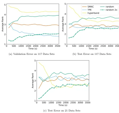
Results: The results on all 117 data sets in Figure 5(a,b) show that Hyperband
outperforms random search in test error rank despite performing worse in validation error rank. Bayesian methods outperform Hyperbandand random search in test error performance
but also exhibit signs of overfitting to the validation set, as they outperformHyperband
by a larger margin on the validation error rank. Notably, random 2× outperforms all other methods. However, for the subset of 21 data sets, Figure 5(c) shows that Hyperband
outperforms all other searchers on test error rank, including random 2×by a very small margin. While these results are more promising, the effectiveness of Hyperband was
0 500 1000 1500 2000 2500 3000 3500 Time (s)
1 2 3 4 5
Average Rank
(a) Validation Error on 117 Data Sets
0 500 1000 1500 2000 2500 3000 3500
Time (s) 1
2 3 4 5
Average Rank
SMAC TPE hyperband
random random 2x
(b) Test Error on 117 Data Sets
0 500 1000 1500 2000 2500 3000 3500
Time (s) 1
2 3 4 5
Average Rank
(c) Test Error on 21 Data Sets
Figure 5: Average rank across all data sets for each searcher. For each data set, the searchers are ranked according to the average validation/test error across 20 trials.
high relative to total training time, while for larger data sets, only a handful of configurations could be trained within the hour window.
We note that while average rank plots like those in Figure 5 are an effective way to aggregate information across many searchers and data sets, they provide no indication about themagnitude of the differences between the performance of the methods. Figure 6, which charts the difference between the test error for each searcher and that of random search across all 117 datasets, highlights the small difference in the magnitude of the test errors across searchers.
smac hyperopt hyperband Searcher
-2.00% -1.50% -1.00% -0.50% 0.00% 0.50% 1.00% 1.50% 2.00%
Difference in Test Error vs Random
Figure 6: Each line plots, for a single data set, the difference in test error versus random search for each search, where lower is better. Nearly all the lines fall within the -0.5% and 0.5% band and, with the exception of a few outliers, the lines are mostly
flat.
promising distribution from which to sample configurations as input into Hyperbandis a
direction for future work.
4.2.2 Kernel Regularized Least Squares Classification
For this benchmark, we tuned the hyperparameters of a kernel-based classifier on CIFAR-10. We used the multi-class regularized least squares classification model, which is known to have comparable performance to SVMs (Rifkin and Klautau, 2004; Agarwal et al., 2014) but can be trained significantly faster.10 The hyperparameters considered in the search space include preprocessing method, regularization, kernel type, kernel length scale, and other kernel specific hyperparameters (see Appendix A for more details). For Hyperband, we
set R= 400, with each unit of resource representing 100 datapoints, andη = 4 to yield a total of 5 brackets. Each hyperparameter optimization algorithm was run for ten trials on Amazon EC2 m4.2xlargeinstances; for a given trial, Hyperband was allowed to run for
two outer loops, brackets= 4 was repeated 10 times, and all other searchers were run for 12 hours.
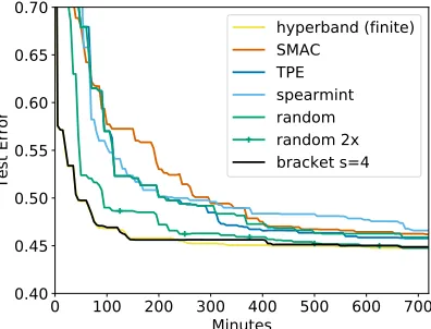
Figure 7 shows that Hyperband returned a good configuration after completing the
firstSuccessiveHalvingbracket in approximately 20 minutes; other searchers failed to
reach this error rate on average even after the entire 12 hours. Notably,Hyperband was
able to evaluate over 250 configurations in this first bracket of SuccessiveHalving, while
competitors were able to evaluate only three configurations in the same amount of time. Consequently,Hyperband is over 30×faster than Bayesian optimization methods and 70×
faster than random search. Brackets= 4 sightly outperformsHyperbandbut the terminal
0 100 200 300 400 500 600 700 Minutes
0.40 0.45 0.50 0.55 0.60 0.65 0.70
Test Error
hyperband (finite) SMAC
TPE random random 2x bracket s=4
Figure 7: Average test error of the best ker-nel regularized least square clas-sification model found by each searcher on CIFAR-10. The color coded dashed lines indicate when the last trial of a given searcher finished.
0 100 200 300 400 500 600 700
Minutes 0.40
0.45 0.50 0.55 0.60 0.65 0.70
Test Error
hyperband (finite) SMAC
TPE spearmint random random 2x bracket s=4
Figure 8: Average test error of the best random features model found by each searcher on CIFAR-10. The test error for Hyperband and
bracket s = 4 are calculated in every evaluation instead of at the end of a bracket.
performance for the two algorithms are the same. Random 2× is competitive with SMAC and TPE.
4.3 Feature Subsampling to Speed Up Approximate Kernel Classification
Next, we examine the performance of Hyperband when using features as a resource on a
random feature kernel approximations task. Features were randomly generated using the method described in Rahimi and Recht (2007) to approximate the RBF kernel, and these random features were then used as inputs to a ridge regression classifier. The hyperparameter search space included the preprocessing method, kernel length scale, andL2 penalty. While it
may seem natural to use infinite horizonHyperband, since the fidelity of the approximation
improves with more random features, in practice, the amount of available machine memory imposes a natural upper bound on the number of features. Thus, we used finite horizion
Hyperband with a maximum resource of 100k random features, which comfortably fit
into a machine with 60GB of memory. Additionally, we set one unit of resource to be 100 features, so R= 1000. Again, we set η= 4 to yield 5 brackets of SuccessiveHalving. We
ran 10 trials of each searcher, with each trial lasting 12 hours on an1-standard-16 machine from Google Cloud Compute. The results in Figure 8 show that Hyperband is around
6×faster than Bayesian methods and random search. Hyperbandperforms similarly to
bracket s= 4. Random 2×outperforms Bayesian optimization algorithms.
4.4 Experimental Discussion
While our experimental results show Hyperbandis a promising algorithm for
1. What impacts the speedups provided by Hyperband?
2. Why doesSuccessiveHalving seem to outperform Hyperband?
3. What about hyperparameters that should depend on the resource?
We next address each of these questions in turn.
4.4.1 Factors Impacting the Performance of Hyperband
For a givenR, the most exploratorySuccessiveHalvinground performed by Hyperband
evaluatesR configurations using a budget of (blogη(R)c+ 1)R, which gives an upper bound on the potential speedup over random search. If training time scales linearly with the resource, the maximum speedup offered by Hyperband compared to random search is
R
(blogη(R)c+1). For the values of η and R used in our experiments, the maximum speedup
over random search is approximately 50×given linear training time. However, we observe a range of speedups from 6× to 70×faster than random search. The differences in realized speedup can be explained by three factors:
1. How training time scales with the given resource. In cases where training time is superlinear as a function of the resource, Hyperbandcan offer higher speedups. For
instance, if training scales like a polynomial of degreep >1, the maximum speedup for
Hyperbandover random search is approximately η
p−1
ηp−1R. In the kernel least square
classifier experiment discussed in Section 4.2.2, the training time scaled quadratically as a function of the resource, which explains why the realized speedup of 70×is higher than the maximum expected speedup given linear scaling.
2. Overhead costs associated with training. Total evaluation time also depends on fixed overhead costs associated with evaluating each hyperparameter configuration, e.g., initializing a model, resuming previously trained models, and calculating validation error. For example, in the downsampling experiments on 117 data sets presented in Section 4.2.1, Hyperband did not provide significant speedup because many data
sets could be trained in a matter of a few seconds and the initialization cost was high relative to training time.
3. The difficulty of finding a good configuration. Hyperparameter optimization problems can vary in difficulty. For instance, an ‘easy’ problem is one where a randomly sampled configuration is likely to result in a high-quality model, and thus we only need to evaluate a small number of configurations to find a good setting. In contrast, a ‘hard’ problem is one where an arbitrary configuration is likely to be bad, in which case many configurations must be considered. Hyperband leverages downsampling to
boost the number of configurations that are evaluated, and thus is better suited for ‘hard’ problems where more evaluations are actually necessary to find a good setting.
only 6×faster than random search. In contrast, for the neural network experiments in Section 4.1, we hypothesize that faster speedups are observed forHyperbandbecause
the dimension of the search space is higher.
4.4.2 Comparison to SuccessiveHalving
With the exception of the LeNet experiment (Section 3.3) and the 117 Datasets experi-ment (Section 4.2.1), the most aggressive bracket of SuccessiveHalving outperformed Hyperband in all of our experiments. In hindsight, we should have just run brackets= 4,
since aggressive early-stopping provides massive speedups on many of these benchmarking tasks. However, as previously mentioned, it was unknown a priori that bracket s = 4 would perform the best and that is why we have to cycle through all possible brackets with Hyperband. Another question is what happens when one increases seven further,
i.e. instead of 4 rounds of elimination, why not 5 or even more with the same maximum resource R? In our case, s = 4 was the most aggressive bracket we could run given the minimum resource per configuration limits imposed for the previous experiments. However, for larger data sets, it is possible to extend the range of possible values fors, in which case,
Hyperbandmay either provide even faster speedups if more aggressive early-stopping helps
or be slower by a small factor if the most aggressive brackets are essentially throwaways.
We believe prior knowledge about a task can be particularly useful for limiting the range of brackets explored by Hyperband. In our experience, aggressive early-stopping
is generally safe for neural network tasks and even more aggressive early-stopping may be reasonable for larger data sets and longer training horizons. However, when pushing the degree of early-stopping by increasings, one has to consider the additional overhead cost associated with examining more models. Hence, one way to leverage meta-learning would be to use learning curve convergence rate, difficulty of different search spaces, and overhead costs of related tasks to determine the brackets considered by Hyperband.
4.4.3 Resource Dependent Hyperparameters
In certain cases, the setting for a given hyperparameter should depend on the allocated resource. For example, the maximum tree depth regularization hyperparameter for random forests should be higher with more data and more features. However, the optimal tradeoff between maximum tree depth and the resource is unknown and can be data set specific. In these situations, the rate of convergence to the true loss is usually slow because the performance on a smaller resource is not indicative of that on a larger resource. Hence, these problems are particularly difficult forHyperband, since the benefit of early-stopping
can be muted. Again, while Hyperband will only be a small factor slower than that
of SuccessiveHalving with the optimal early-stopping rate, we recommend removing
5. Theory
In this section, we introduce the pure-exploration non-stochastic infinite-armed bandit (NIAB) problem, a very general setting which encompasses our hyperparameter optimization problem of interest. As we will show, Hyperband is in fact applicable to problems far beyond just hyperparameter optimization. We begin by formalizing the hyperparameter optimization problem and then reducing it to the pure-exploration NIAB problem. We subsequently present a detailed analysis of Hyperband in both the infinite and finite
horizon settings.
5.1 Hyperparameter Optimization Problem Statement
LetX denote the space of valid hyperparameter configurations, which could include contin-uous, discrete, or categorical variables that can be constrained with respect to each other in arbitrary ways (i.e. X need not be limited to a subset of [0,1]d). For k = 1,2, . . . let
`k: X → [0,1] be a sequence of loss functions defined over X. For any hyperparameter
configurationx∈ X,`k(x) represents the validation error of the model trained usingxwithk
units of resources (e.g. iterations). In addition, for someR∈N∪ {∞}, define`∗ = limk→R`k
and ν∗ = infx∈X`∗(x). Note that `k(·) for allk ∈N, `∗(·), andν∗ are all unknown to the
algorithm a priori. In particular, it is uncertain how quickly `k(x) varies as a function of x
for any fixed k, and how quickly`k(x)→`∗(x) as a function of kfor any fixed x∈ X.
We assume hyperparameter configurations are sampled randomly from a known probabil-ity distributionp(x) :X →[0,∞), with support onX. In our experiments,p(x) is simply the uniform distribution, but the algorithm can be used with any sampling method. IfX∈ X
is a random sample from this probability distribution, then `∗(X) is a random variable whose distribution is unknown since `∗(·) is unknown. Additionally, since it is unknown how
`k(x) varies as a function ofx or k, one cannot necessarily infer anything about`k(x) given
knowledge of `j(y) for any j∈N,y ∈ X. As a consequence, we reduce the hyperparmeter
optimization problem down to a much simpler problem that ignores all underlying structure of the hyperparameters: we only interact with some x∈ X through its loss sequence `k(x)
for k= 1,2, . . .. With this reduction, the particular value ofx∈ X does nothing more than index or uniquely identify the loss sequence.
Without knowledge of how fast `k(·) → `∗(·) or how`∗(X) is distributed, the goal of Hyperbandis to identify a hyperparameter configuration x∈ X that minimizes`∗(x)−ν∗
by drawing as many random configurations as desired while using as few total resources as possible.
5.2 The Pure-Exploration Non-stochastic Infinite-Armed Bandit Problem
We now formally define the bandit problem of interest, and relate it to the problem of hyperparameter optimization. Each “arm” in the NIAB game is associated with a sequence that is drawn randomly from a distribution over sequences. If we “pull” the ith drawn arm exactlyktimes, we observe a loss `i,k. At each time, the player can either draw a new arm
i(i.e. we have no side-knowledge or feature representation of an arm), and we also make the following two additional assumptions:
Assumption 1 For each i∈N the limit limk→∞`i,k exists and is equal to νi.11
Assumption 2 Each νi is a bounded i.i.d. random variable with cumulative distribution functionF.
The objective of the NIAB problem is to identify an arm ˆıwith small νˆı using as few total
pulls as possible. We are interested in characterizing νˆı as a function of the total number of
pulls from all the arms. Clearly, the hyperparameter optimization problem described above is an instance of the NIAB problem. In this case, arm i correspondes to a configuration
xi ∈ X, with`i,k =`k(xi); Assumption 1 is equivalent to requiring thatνi =`∗(xi) exists;
and Assumption 2 follows from the fact that the arms are drawn i.i.d. from X according to distribution function p(x). F is simply the cumulative distribution function of `∗(X), where X is a random variable drawn from the distribution p(x) overX. Note that since the arm draws are independent, the νi’s are also independent. Again, this is not to say that the
validation losses do not depend on the settings of the hyperparameters; the validation loss could well be correlated with certain hyperparameters, but this is not used in the algorithm and no assumptions are made regarding the correlation structure.
In order to analyze the behavior of Hyperbandin the NIAB setting, we must define
a few additional objects. Let ν∗= inf{m:P(ν ≤m)>0}>−∞, since the domain of the
distributionF is bounded. Hence, the cumulative distribution function F satisfies
P(νi−ν∗≤) =F(ν∗+) (1)
and let F−1(y) = infx{x : F(x) ≤ y}. Define γ:N → R as the pointwise smallest,
monotonically decreasing function satisfying
sup
i
|`i,j−`i,∗| ≤γ(j) , ∀j∈N. (2)
The function γ is guaranteed to exist by Assumption 1 and bounds the deviation from the limit value as the sequence of iterates j increases. For hyperparameter optimization, this follows from the fact that `k uniformly converges to `∗ for all x ∈ X. In addition, γ
can be interpretted as the deviation of the validation error of a configuration trained on a subset of resources versus the maximum number of allocatable resources. Finally, define
R as the first index such that γ(R) = 0 if it exists, otherwise set R = ∞. For y ≥0 let
γ−1(y) = min{j∈N:γ(j)≤y}, using the convention that γ−1(0) :=R which we recall can be infinite.
As previously discussed, there are many real-world scenarios in which R is finite and known. For instance, if increasing subsets of the full data set is used as a resource, then the maximum number of resources cannot exceed the full data set size, and thusγ(k) = 0 for all k≥R where R is the (known) full size of the data set. In other cases such as iterative training problems, one might not want to or know how to boundR. We separate these two settings into the finite horizon setting whereR is finite and known, and the infinite horizon
SuccessiveHalving (Infinite horizon)
Input: BudgetB,narms where`i,k denotes the kth loss from theith arm Initialize: S0= [n].
Fork= 0,1, . . . ,dlog2(n)e −1
Pull each arm inSk forrk=b|Sk|dlogB
2(n)ec
times.
Keep the bestb|Sk|/2carms in terms of the rkth observed loss asSk+1.
Output: ˆı,`
ˆı,b B/2 dlog2(n)ec
where ˆı=Sdlog2(n)e
Hyperband (Infinite horizon) Input: None
Fork= 1,2, . . .
Fors∈Ns.t. k−s≥log2(s)
Bk,s= 2k,nk,s= 2s
ˆık,s, `
ˆ
ık,s,b
2k−1
s c
←SuccessiveHalving(Bk,s,nk,s)
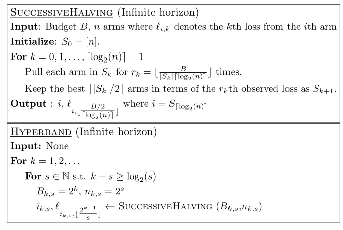
Figure 9: (Top) TheSuccessiveHalving algorithm proposed and analyzed in Jamieson
and Talwalkar (2015) for the non-stochastic setting. Note this algorithm was originally proposed for the stochastic setting in Karnin et al. (2013). (Bottom) The Hyperband algorithm for the infinite horizon setting. Hyperband calls SuccessiveHalvingas a subroutine.
setting where no bound onR is known and it is assumed to be infinite. While our empirical results suggest that the finite horizon may be more practically relevant for the problem of hyperparameter optimization, the infinite horizon case has natural connections to the literature, and we begin by analyzing this setting.
5.3 Infinite Horizon Setting (R =∞)
Consider the Hyperbandalgorithm of Figure 9. The algorithm usesSuccessiveHalving
(Figure 9) as a subroutine that takes a finite set of arms as input and outputs an estimate of the best performing arm in the set. We first analyze SuccessiveHalving(SH) for a
given set of limits νi and then consider the performance of SH whenνi are drawn randomly
according toF. We then analyze theHyperbandalgorithm. We note that the algorithm of
Theorem 1 Fix narms. Let νi= lim
τ→∞`i,τ and assume ν1 ≤ · · · ≤νn. For any >0 let zSH = 2dlog2(n)e max
i=2,...,ni(1 +γ
−1 max
4, νi−ν1
2 )
≤2dlog2(n)e n+ X
i=1,...,n
γ−1 max4,νi−ν1 2
If the SuccessiveHalving algorithm of Figure 9 is run with any budgetB > zSH then an armˆı is returned that satisfies νˆı−ν1≤/2. Moreover,|`
ˆı,bdlogB/2 2(n)ec
−ν1| ≤.
The next technical lemma will be used to characterize the problem dependent term P
i=1,...,nγ−1 max
4, νi−ν1
2 when the sequences are drawn from a probability distribution. Lemma 2 Fix δ ∈(0,1). Let pn= log(2n/δ). For any≥4(F−1(pn)−ν∗) define
H(F, γ, n, δ, ) := 2n
Z ∞
ν∗+/4
γ−1(t−ν∗
4 )dF(t) + 4
3log(2/δ) + 2nF(ν∗+/4)
γ−1 16
and H(F, γ, n, δ) :=H(F, γ, n, δ,4(F−1(p
n)−ν∗)) so that
H(F, γ, n, δ) = 2n
Z 1
pn
γ−1(F−1(t)−ν∗ 4 )dt+
10
3 log(2/δ)γ
−1F−1(pn)−ν∗ 4
.
For narms with limits ν1≤ · · · ≤νn drawn fromF, then
ν1 ≤F−1(pn) and n
X
i=1
γ−1 max
4, νi−ν1
2 ≤H(F, γ, n, δ, ) for any≥4(F−1(pn)−ν∗) with probability at least 1−δ.
Setting = 4(F−1(pn) −ν∗) in Theorem 1 and using the result of Lemma 2 that
ν∗ ≤ν1 ≤ν∗+ (F−1(pn)−ν∗), we immediately obtain the following corollary.
Corollary 3 Fix δ∈(0,1) and≥4(F−1(log(2n/δ))−ν∗). Let B = 4dlog2(n)eH(F, γ, n, δ, )
where H(F, γ, n, δ, ) is defined in Lemma 2. If the SuccessiveHalving algorithm of Figure 9 is run with the specified B and n arm configurations drawn randomly according to F, then an arm ˆı ∈ [n] is returned such that with probability at least 1−δ we have
νˆı −ν∗ ≤ F−1(log(2n/δ))−ν∗
+/2. In particular, if B = 4dlog2(n)eH(F, γ, n, δ) and
= 4(F−1(log(2n/δ))−ν∗) thenνˆı−ν∗ ≤3 F−1(log(2n/δ))−ν∗
with probability at least 1−δ.
Note that for any fixed n∈Nwe have for any ∆>0
P( min
i=1,...,nνi−ν∗≥∆) = (1−F(ν∗+ ∆))
n≈e−nF(ν∗+∆)
which implies E[mini=1,...,nνi−ν∗]≈F−1(n1)−ν∗. That is,n needs to be sufficiently large
5.3.1 Non-Adaptive Uniform Allocation
The non-adaptive uniform allocation strategy takes as inputs a budget B and n arms, allocatesB/n to each of the arms, and picks the arm with the lowest loss. The following results allow us to compare withSuccessiveHalving.
Proposition 4 Suppose we draw n random configurations from F, train each with j = min{B/n, R}iterations, and letˆı= arg mini=1,...,n`j(Xi). Without loss of generality assume
ν1 ≤. . .≤νn. If
B ≥nγ−112(F−1(log(1n/δ))−ν∗) (3)
then with probability at least 1−δ we have νˆı−ν∗ ≤2
F−1log(1n/δ)−ν∗. In contrast, there exists a sequence of functions`j that satisfyF and γ such that if
B ≤nγ−12(F−1(n+log(log(c/δc/δ)))−ν∗)
then with probability at least δ, we have νˆı −ν∗ ≥ 2(F−1(n+log(log(c/δc/δ)))−ν∗), where c is a constant that depends on the regularity of F.
For any fixed nand sufficiently largeB, Corollary 3 shows that SuccessiveHalving
outputs an ˆı∈[n] that satisfiesνˆı−ν∗ .F−1(log(2n/δ))−ν∗ with probability at least 1−δ.
This guarantee is similar to the result in Proposition 4. However, SuccessiveHalving
achieves its guarantee as long as12
B 'log2(n) "
log(1/δ)γ−1F−1(log(1n/δ))−ν∗+n
Z 1
log(1/δ)
n
γ−1(F−1(t)−ν∗)dt
#
, (4)
and this sample complexity may be substantially smaller than the budget required by uniform allocation shown in Eq. (3) of Proposition 4. Essentially, the first term in Eq. (4) represents the budget allocated to the constant number of arms with limitsνi≈F−1(log(1n/δ)) while
the second term describes the number of times the sub-optimal arms are sampled before discarded. The next section uses a particular parameterization for F andγ to help better illustrate the difference between the sample complexity of uniform allocation (Equation 3) versus that of SuccessiveHalving (Equation 4).
5.3.2 A Parameterization of F and γ for Interpretability
To gain some intuition and relate the results back to the existing literature, we make explicit parametric assumptions onF andγ. We stress that all of our results hold for generalF and
γ as previously stated, and this parameterization is simply a tool to provide intuition. First assume that there exists a constant α >0 such that
γ(j)'
1
j
1/α
. (5)
Note that a large value of α implies that the convergence of`i,k →νi is very slow.
We will consider two possible parameterizations of F. First, assume there exists positive constantsβ such that
F(x)'
(x−ν∗)β ifx≥ν∗
0 ifx < ν∗
. (6)
Here, a large value of β implies that it is very rare to draw a limit close to the optimal valueν∗. The same model was studied in Carpentier and Valko (2015). Fix some ∆>0. As discussed in the preceding section, if n= Flog(1(ν /δ)
∗+∆) '∆
−βlog(1/δ) arms are drawn from
F then with probability at least 1−δ we have mini=1,...,nνi ≤ν∗+ ∆. Predictably, both
uniform allocation andSuccessiveHalvingoutput aνˆı that satisfiesνˆı−ν∗.
log(1/δ)
n
1/β with probability at least 1−δ provided their measurement budgets are large enough. Thus, ifn'∆−βlog(1/δ) and the measurement budgets of the uniform allocation (Equation 3) and SuccessiveHalving (Equation 4) satisfy
Uniform allocation B'∆−(α+β)log(1/δ)
SuccessiveHalving B'log2(∆−βlog(1/δ))
∆−αlog(1/δ) +∆
−β −∆−α
1−α/β log(1/δ)
'log(∆−1log(1/δ)) log(∆−1) ∆−max{β,α}log(1/δ)
then both also satisfy νˆı−ν∗ .∆ with probability at least 1−δ.13 SuccessiveHalving’s
budget scales like ∆−max{α,β}, which can be significantly smaller than the uniform allocation’s budget of ∆−(α+β). However, because α and β are unknown in practice, neither method knows how to choose the optimaln orB to achieve this ∆ accuracy. In Section 5.3.3, we show how Hyperbandaddresses this issue.
The second parameterization of F is the following discrete distribution:
F(x) = 1
K
K
X
j=1
1{x≤µj} with ∆j :=µj−µ1 (7)
for some set of unique scalarsµ1 < µ2<· · ·< µK. Note that by lettingK→ ∞this discrete
CDF can approximate any piecewise-continuous CDF to arbitrary accuracy. In particular, this model can have multiple means take the same value so that α mass is onµ1 and 1−α
mass is on µ2> µ1, capturing the stochastic infinite-armed bandit model of Jamieson et al.
(2016). In this setting, both uniform allocation andSuccessiveHalving output aνˆı that
is within the top log(1n/δ) fraction of the K arms with probability at least 1−δ if their budgets are sufficiently large. Thus, let q >0 be such that n'q−1log(1/δ). Then, if the measurement budgets of the uniform allocation (Equation 3) and SuccessiveHalving