Cost-Sensitive Learning with Noisy Labels
Nagarajan Natarajan [email protected]∗
Microsoft Research, Bangalore 560001, INDIA
Inderjit S. Dhillon [email protected]
Dept. of Computer Science University of Texas at Austin Austin, TX 78701
Pradeep Ravikumar [email protected]
Machine Learning Dept. Carnegie Mellon University Pittsburgh, PA 15213
Ambuj Tewari [email protected]
Dept. of Statistics, and
Dept. of Electrical Engineering and Computer Science University of Michigan
Ann Arbor, MI 48109
Editor:Guy Lebanon
Abstract
We study binary classification in the presence ofclass-conditional random noise, where the learner gets to see labels that are flipped independently with some probability, and where the flip probability depends on the class. Our goal is to devise learning algorithms that are efficient and statistically consistent with respect to commonly used utility measures. In particular, we look at a family of measures motivated by their application in domains where cost-sensitive learning is necessary (for example, when there is class imbalance). In contrast to most of the existing literature on consistent classification that are limited to the classical 0-1 loss, our analysis includes more general utility measures such as the AM measure (arithmetic mean of True Positive Rate and True Negative Rate). For this problem of cost-sensitive learning under class-conditional random noise, we develop two approaches that are based on suitably modifying surrogate losses. First, we provide a simple unbiased estimator of any loss, and obtain performance bounds for empirical utility maximization in the presence of i.i.d. data with noisy labels. If the loss function satisfies a simple symmetry condition, we show that using unbiased estimator leads to an efficient algorithm for empiri-cal maximization. Second, by leveraging a reduction of risk minimization under noisy labels to classification with weighted 0-1 loss, we suggest the use of a simple weighted surrogate loss, for which we are able to obtain strong utility bounds. This approach implies that methods already used in practice, such as biased SVM and weighted logistic regression, are provably noise-tolerant. For two practically important measures in our family, we show
∗. The work in this manuscript was done when the author was a graduate student at the University of Texas at Austin.
c
that the proposed methods are competitive with respect to recently proposed methods for dealing with label noise in several benchmark data sets.
Keywords: class-conditional label noise, statistical consistency, cost-sensitive learning
1. Introduction
Learning from noisy training data is a problem of theoretical as well as practical interest in machine learning. In many applications such as learning to classify images, it is often the case that the labels are noisy. Even human labelers are susceptible to errors in labeling; for instance, certain image categories may be hard to discern. Designing learning algorithms that help maximize a desired performance measure in such noisy settings, and understanding their statistical consistency properties are the objectives of our current work.
One of the earliest known attempts at learning in the presence of label noise was by Bylander (1994) that concerned learnability of linear threshold functions (LTFs) in the Probably Approximately Correct (PAC) model. In particular, he showed that if the noise rate is uniform and if there is a sufficient margin under the clean distribution, then it is pos-sible to PAC-learn LTFs. He also extended the result to a more realistic noise model called monotonic noise (Bylander, 1998), where the noise rate is allowed to vary per example, but is assumed to be a monotonic function of the distance of the example from the true hyper-plane. Blum and Mitchell (1998), and later Cohen (1997) improved the PAC-learnability results of Bylander (1994) showing that linear threshold functions are efficiently learnable without the margin requirement in the uniform label noise model. A Bayesian approach to the problem of noisy labels is taken by Graepel and Herbrich (2000) and Lawrence and Sch¨olkopf (2001). Cesa-Bianchi et al. (2011) focus on online learning algorithms where only unbiased estimates of the gradient of the loss are needed to provide guarantees for learning with noisy data. However, they consider a much harder noise model where instancesas well as labels are noisy. Because of the harder noise model, they necessarily require multiple noisy copies per clean example and the unbiased estimation schemes also become fairly complicated, particularly for non-smooth classification losses such as the hinge loss.
In order to more clearly understand the impact of label noise, it is useful to consider a more natural and simpler formalism for label noise, where a random noise process cor-rupts the labels (Biggio et al., 2011), which otherwise arise from some “clean” distribution. There has been a long line of work in the theoretical machine learning community on such formalisms. Soon after the introduction of the noise-free PAC model, Angluin and Laird (1988) proposed the random classification noise (RCN) model where each label is flipped independently with some probability ρ ∈ [0,1/2). It is known (Aslam and Decatur, 1996; Cesa-Bianchi et al., 1999) that finiteness of the VC dimension characterizes learnability in the RCN model. Similarly, in the online mistake bound model, the parameter that charac-terizes learnability without noise — the Littlestone dimension — continues to characterize learnability even in the presence of random label noise (Ben-David et al., 2009). These results are for the so-called 0-1 loss: if the true label is y ∈ {−1,+1} and the prediction is t, the 0-1 loss defined as `0-1(y, t) = 1{yt≤0} (where 1{P} denotes the indicator function
2013). A great deal of practical work has also been done on the problem; see, for instance, the survey article by Nettleton et al. (2010).
In this paper, we consider theclass-conditional random label noise (abbreviated CCN) setting. Here, the data consists of iid samples drawn from a noisy version Dρ of an
under-lying “clean” distribution D, and where the noise rates depend on the class label. To the best of our knowledge, general results in this setting have not been obtained before. We note that developing guarantees in the presence of CCN label noise also has implications in varied partially-supervised settings such as learning from only positive and unlabeled data (Elkan and Noto, 2008), which can be cast under this setting. For the theoretical results presented in this work, we assume that the true noise rates (that characterize Dρ)
are known. In practice, one may use the domain knowledge to provide an estimate for noise rates (see Section 6.3), or use a plug-in estimator for noise rates such as the one prescribed by Scott (2015).
A key facet of the classification problem is the evaluation metric which captures discrep-ancy between the predicted label and the true label, and which we would want to minimize (or correspondingly, an evaluation utility measure which we would want to maximize). While classification accuracy is a popular utility measure, many other performance mea-sures have also been considered in practice. One important family of meamea-sures constitutes cost-sensitive learning, and is motivated by applications and domains where misclassifica-tion cost could depend on the category of the example. For example, in disease diagnosis, false positives and false negatives often have very different associated impacts. Most, if not all, of the existing theoretical work on classification focuses on obtaining consistent learning algorithms for the 0-1 loss or its surrogates. In this paper, we consider a general class of util-ity measures that can be expressed as a linear combination of the entries of the “confusion matrix,” namely, true positives, true negatives, false positives and false negatives.
Towards this problem of learning classifiers with respect to general utility measures and class conditional label noise, we develop two methods for suitably modifyingany given
surrogate loss function `, and show that minimizing the sample average of the modified
proxy loss function ˜`leads to provable utility bounds where the utility is calculated on the clean distribution.
In our first approach, the modified or proxy loss is an unbiased estimate of the loss func-tion associated with the utility measure of interest. The idea of using unbiased estimators is well-known in stochastic optimization (Nemirovski et al., 2009). Nonetheless, we bring out some important aspects of using unbiased estimators of loss functions for empirical utility maximization under CCN. In particular, we give a simple symmetry condition on the loss (enjoyed, for instance, by the Huber, logistic, and squared losses) to ensure that the proxy loss is also convex. Hinge loss does not satisfy the symmetry condition, and thus leads to a non-convex problem. We nonetheless provide a convex surrogate, leveraging the fact that the non-convex hinge problem is “close” to a convex problem (Theorem 12). This is strikingly different from the online learning setting (examined in Section 4) that requires only the expected loss to be convex.
the weights are label-dependent, as the proxy loss function. Our analysis builds on the notion of consistency of weighted loss functions studied by Scott (2012). This approach leads to a remarkable result that appropriately weighted losses like biased SVMs studied by Liu et al. (2003) are robust to CCN.
The key contributions of the paper are summarized below:
1. We develop methods for learning, that are provably consistent, (a) in the presence of asymmetric label noise, and (b) with respect to general cost-sensitive utility measures beyond the classical 0-1 loss.
2. To the best of our knowledge, we are the first to provide guarantees for cost-sensitive learning under random label noise in the general setting of convex surrogates, without any assumptions on the true distribution.
3. As one consequence of our results, we resolve an elusive theoretical gap in the under-standing of practical methods like biased SVM and weighted logistic regression: as we show, they are provably noise-tolerant (Theorem 18). We obtain the result as a consequence of being able to linearly relate the risk w.r.t. a weighted 0-1 loss under the noisy distribution to that w.r.t. the 0-1 loss under the clean distribution (Theorem 16).
4. Our proxy losses are easy to compute: the proposed approaches yield efficient algo-rithms.
5. Experiments on benchmark data sets show that the methods are robust even at high noise rates, for maximizing different performance measures from our family.
In a preliminary version of the paper (Natarajan et al., 2013), we provided guarantees for risk minimization (using the 0-1 loss) in the presence of class-conditional label noise. In this paper, we provide a more general and detailed treatment of the theory, by character-izing the optimal classifiers under more general performance measures used in practice (in Sections 4 and 5). We extend our earlier approach (Natarajan et al., 2013) to cost-sensitive learning (Section 3.2). Our results in this paper also serve to generalize some of the known consistency results for performance measures such as the AM measure, even in the noise-free setting.
We now expand on the organization of the paper. We begin by discussing some closely related work in Section 2. We introduce and set the problem up formally in Section 3. The class-conditional noise model is specified by two parametersρ+1 and ρ−1 which correspond
showed consistency of certain empirical estimation algorithms for the AM measure (defined in Proposition 1). An important result that connects the excess risk of a decision function (in terms of the 0-1 loss),R(f)−minfR(f), and its “utility deficit”, maxfU(f)− U(f), is
established in Lemma 3. As a consequence of this result, we are able to use the surrogates for 0-1 loss for empirical estimation, in order to maximize cost-sensitive measures.
We describe our first approach of using unbiased surrogate loss functions in Section 4. Here, the idea is to construct an unbiased estimator of a given loss function (a surrogate of the 0-1 loss). The unbiased estimator involves the noise rates ρ+1 and ρ−1. For optimizing
a given utility measure U, we propose an empirical risk minimization procedure based on the unbiased surrogate thus obtained. We establish utility deficit bounds for the resulting empirical estimator in Theorem 9. Here, we also look at the online learning setting, where examples arrive sequentially (with noisy labels), and obtain similar consistency guarantees. Our second approach is detailed in Section 5. The key observation is that the optimal decision function for utilityU in our family with respect to the noisy distribution is simply given by thresholding P(Y = 1|x) with respect to theclean distribution, at a certain value that depends only on the distribution and the measure U itself. This enables us to use a weighted surrogate of the 0-1 loss, where the weights depend on the measure U and noise ratesρ+1 andρ−1. We provide rigorous guarantees for consistency of the resulting empirical
estimator in Theorem 18.
We present detailed experimental results that support our theory in Section 6. We per-form experiments on synthetic and benchmark data sets, on both the proposed approaches. We compare to state-of-the-art algorithms for learning with noisy data on different data sets and different noise settings. We use two performance measures in experiments: classifica-tion accuracy and the AM measure, as representatives of the family of measures considered in the paper.
2. Related Work
Manwani and Sastry (2013) consider whether empirical risk minimization of the loss itself on the noisy data is a good idea when the goal is to obtain small risk under the clean distribution. But the answer is affirmative only for 0-1 and squared losses. Therefore, if empirical risk minimization over noisy samples has to work, we necessarily have to change the loss used to calculate the empirical risk. More recently, Ghosh et al. (2014) prove that a loss function`satisfying the symmetry condition`(f(x),1) +`(f(x),−1) =C,∀x,∀f for some constantC are noise-tolerant, under the assumption that the classes are separable un-der the clean distribution (here,`is said to benoise-tolerant ifE(X,Y)∼D
`0-1(f`∗(X), Y)
=
E(X,Y)∼D
`0-1( ˜f`∗(X), Y)
, wheref`∗ and ˜f`∗ denote the minimizers of`-risk under clean and noisy distribution respectively). Furthermore, they show that by choosing a sufficiently large value of a parameter in the loss functions such as sigmoid loss, ramp loss and probit loss, the losses can be made tolerant to non-uniform label noise (i.e. noise rate is allowed to depend on the example) as well. Unfortunately, the aforementioned loss functions are all non-convex, and convex losses used in practice do not satisfy the sufficiency conditions. It remains an open question if the symmetry condition is indeed necessary for noise tolerance, at least under the separability assumption.
van Rooyen and Williamson (2015) extend the idea behind the method of unbiased estimators to more general learning settings beyond binary classification. For example, they consider semi-supervised learning, classification with more than two classes, and learning with partial labels (a partial label is aset of labels containing the true label).
Scott et al. (2013) also study the problem of learning classifiers under the class-conditional noise model. However, they approach the problem from a different set of assumptions — the noise rates arenot known, and the true distribution satisfies a certain “mutual irreducibil-ity” property. They model the observed noisy instances as arising from “contaminated” mixtures of positive and negative classes and show that the mixture proportions can be con-sistently estimated by maximal denoising of the noisy distributions. Blanchard and Scott (2014) establish similar results for the multi-class classification problem. Scott (2015) pro-vides a consistent estimator with convergence rates for the cost parameterαin our weighted surrogate loss (Equation 2). In this paper, however, we selectαby cross-validation and also examine the sensitivity of selectingα (in Section 6.3).
3. Preliminaries
LetD be the underlying true distribution generating (X, Y)∈ X × {±1} pairs from which
niid samples (X1, Y1), . . . ,(Xn, Yn) are drawn. Let η(X) =P(Y = 1|X) under D. 3.1 Class-conditional Noise
After injecting random classification noise (independently for each i) into these samples, corrupted samples (X1,Y˜1), . . . ,(Xn,Y˜n) are obtained. The class-conditional random noise
model (CCN, for short) is given by:
P( ˜Y =−1|Y = +1) =ρ+1, P( ˜Y = +1|Y =−1) =ρ−1, and
The corrupted samples are what the learning algorithm sees. We will assume that the noise rates ρ+1 and ρ−1 are known to the learner. Let the distribution of (X,Y˜) be Dρ. Noisy
labels are denoted by ˜y. Let ˜η(X) =P( ˜Y = 1|X) under Dρ.
3.2 Cost-sensitive Classification
Letf :X →Rdenote a real-valued decision function. The goal in classification is to learn
f from a training sample, such that some cost or loss measure is minimized. The most common measure is the probability of misclassification, also called therisk, which is simply the expected 0-1 loss defined as
R(f) :=RD(f) :=E(X,Y)∼D
1{sign(f(X))6=Y}
.
Minimizing the 0-1 loss on a training sample, over some class of decision functions, is often intractable. In practice, it is common to minimize asurrogateloss function that is chosen for its computational advantages such as convexity. Minimizing risk (or equivalently, maximiz-ing the accuracy) of a classifier is however not always appropriate, and in fact practitioners have devised many alternative performance metrics to address specific needs of a target domain. Class imbalance is an important scenario where accuracy of classifier is not a good metric to optimize: a trivial classifier that assigns all the examples to the majority class will have a high accuracy. However, little is known about optimal classification or consistent algorithms for binary classification w.r.t. general performance measures, even when the observations are noise-free. An important family of performance measures that is preferred in many scenarios including heavy class imbalance and asymmetry in real-world costs asso-ciated with specific classes constitutes cost-sensitive learning. Cost-sensitive performance measures are given by a weighted combination of the four fundamental population quan-tities associated with the “confusion matrix” - true positives, false positives (also known as type-I error), false negatives (also known as type-II error) and true negatives as defined below:
T P(f;D) =E(X,Y)∼D[1{f(X)=1,Y=1}], T N(f;D) =E(X,Y)∼D[1{f(X)=−1,Y=−1}]
F P(f;D) =E(X,Y)∼D[1{f(X)=1,Y=−1}], F N(f;D) =E(X,Y)∼D[1{f(X)=−1,Y=1}].
We consider the family of measuresU defined by:
U(f;D) =a11T P(f;D) +a10F P(f;D) +a01F N(f;D) +a00T N(f;D), (1)
given constants a0, a11, a10, a01, a00 (that could depend on D). In the remainder of the
paper, U refers to a measure in this family, unless specified otherwise. We will use the terms performance measure andutility measure interchangeably in this paper.
Next, we state two important, commonly-used measures in this family.
Proposition 1 1. The Accuracy measureUAcc(f;D)belongs in the family (1)witha11= a00= 1 and a10=a01= 0.
2. The AM (Arithmetic Mean of TPR and TNR) measure defined as
UAM(f;D) := 1
2 T P R(f;D) +T N R(f;D)
where T P R(f;D) = P(f(X) = 1|Y = 1)is the true positive rate and T N R(f;D) =
P(f(X) = −1|Y = −1) is the true negative rate, belongs in the family (1) with
constants a10=a01= 0, a11= 2(11−π) and a00=
1
2π, where π=P(Y = 1) under D.
3.2.1 Cost-sensitive Classification without Label Noise
Before we present our approaches for cost-sensitive classification under class-conditional label noise, it will be useful to consider the setting without such label noise, and setup appropriate notation. Given a utility measure U and training data, our goal is to learn a decision function f that maximizes U with respect to the clean distribution. The opti-mal decision function (called Bayes optiopti-mal) that maximizesU over all real-valued decision functions is denoted as f?(x) := arg max
fU(f;D). We denote by U∗ the optimal utility
value, i.e. U∗ = U(f?). It is not always possible to characterize the Bayes optimal of ar-bitrary performance measures. Cost-sensitive measures are particularly interesting because their Bayes optimal exhibits a simple form, and as a consequence, consistent algorithms are readily obtained in practice in the noise-free case. Bayes optimal classifier for the family (1) is characterized in the following Lemma. Recall thatη(x) =P(Y = 1|x) underD.
Lemma 2 The Bayes optimal of any measure U in family (1)is given by
arg max
f U(f;D) = sign(η(x)−δ ∗ D),
where the threshold is defined as
δ∗D = a00−a10
a00−a10−a01+a11 .
The proof is simple and can be found elsewhere (Elkan, 2001). It is well-known that accuracy UAcc(f;D) is maximized by sign(η(x)−1/2) which is also readily obtained by applying the above lemma. For the AM measure UAM(f;D), one easily verifies that the threshold is
π=P(Y = 1).
For any general measure U, we are interested in controlling the deficit utility which is U∗− U(f;D). The following simple lemma relates the deficit utility for the family (1) to
that of a certain weighted 0-1 risk.
Lemma 3 Define α-weighted risk under distributionD as:
Rα(f) :=Rα,D(f) :=E(X,Y)∼D
(1−α)1{Y=1}1{f(X)≤0}+α1{Y=−1}1{f(X)>0}
.
For any measure U in the family (1):
Rδ∗
D(f)−R ∗ δ∗D =
1
(a11+a00)−(a10+a01)
(U∗− U(f;D)),
where R∗δ∗
D = minfRδ
∗
Proof Letc1 = (a11+a00)−(a10−a01) andc2=a00−a10. From Lemma 2, we knowδ∗D = cc21. Note that 1 > c1 > 0 for otherwise maximizingU would not make sense (See Remark 4),
and therefore 0≤δ∗D ≤1. For any f, let θ denote the classifier θ(x) = sign(f(x)). We can rewrite U(θ) as U(θ) =c1[(1−δD∗)T P +δ∗DT N] + ˜A, where ˜A is a constant. We have:
Rδ∗
D(θ) = E(X,Y)∼D
(1−δD∗)1{Y=1}+δD∗1{Y=0}
.1{θ(X)6=Y}
= (1−δD∗)P(Y = 1, θ(X) =−1) +δ∗DP(Y =−1, θ(X) = 1)
= (1−δD∗)F N +δD∗F P
= (1−δD∗)(π−T P) +δ∗D(1−π−T N)
= (1−δD∗)π+δD∗(1−π)− (1−δD∗)T P +δ∗DT N
= (1−δD∗)π+δD∗(1−π) + A˜
c1
− 1
c1
U(θ).
Observing that (1−δ∗D)π +δ∗D(1−π) + cA˜
1 is a constant independent of θ, the proof is complete.
Remark 4 Note that we can assume (a11+a00)−(a10+a01)>0, otherwise maximizing
U would not make sense. If indeed, (a11+a00)−(a10+a01)<0, then Lemma 3 still holds
but with U∗ interpreted as U∗ = minfU(f;D).
Of course, minimizing the α-weighted risk on a training sample is not tractable. Scott (2012) extends the notion of the classification calibration defined by Bartlett et al. (2006) for the (unweighted) 0-1 loss. The following result of Scott (2012) tells us that by using a similarly weighted surrogate loss function `α, one can control the excess α-weighted risk.
Define `α-risk, R`α,D(f) =E(X,Y)∼D[`α(f(X), Y)], and R ∗
`α = minfR`α,D(f).
Lemma 5 (α-classification calibration (Scott, 2012)) Given a loss function `(t, y),
and α∈(0,1), define theα-weighted loss:
`α(t, y) = (1−α)1{y=1}+α1{y=−1}
`(t, y) . (2)
`α is α-classification calibrated (or α-CC) iff there exists a convex, non-decreasing and
invertible transformationψ`,α, withψ`,α(0) = 0, such that
ψ`,α(Rα(f)−Rα∗)≤R`α,D(f)−R ∗ `α .
In other words, consistency with respect to `α-risk implies consistency with respect to α
-weighted (0-1) risk forα-CC losses. Also, for any`that is classification-calibrated (Bartlett
et al., 2006) (such as logistic, hinge and squared losses), the corresponding `α is α-CC.
If we choose α = δD∗, Lemmas 3 and 5 together guarantee the consistency of using a weighted surrogate loss function in practice, when we obtain samples from the clean distri-bution D. However, if the labels are noisy, the outlined procedure is no longer consistent. One necessarily has to change the loss function ` or rather `α to be able to tolerate the
Remark 6 Most commonly used loss functions such as hinge and logistic losses are (even)
margin losses, i.e. `(t, y) = φ(ty), for some φ : R → [0,∞). We could also consider an
uneven margin loss function of the form:
`(t, y) = 1{y=1}φ(t) + 1{y=−1}βφ(−γt),
for β, γ >0. Scott (2012) showed that for convex φ, the above defined uneven margin loss
` is classification-calibrated, and in turn, the corresponding`α isα-CC, when β= 1γ. Such
uneven margin losses have been used in practice mostly as heuristics as pointed out in (Scott, 2012). Thus, in principle, we could use uneven margin losses, and all the results in this manuscript will hold just the same.
Notation. We use letters with the ‘tilde’ accent to denote noisy versions of quantities or variables, e.g. ˜` is the loss function to be used on the noisy data, and ˜y denotes a noisy label. We useF :X →Rto denote a fixed class of real-valued decision functions. Iff is not quantified in a minimization, then it is implicit that the minimization is over all measurable functions. Instances are denoted by x ∈ X ⊆ Rd. Though most of our results apply to a
general function classF, we instantiateF to be the set of hyperplanes of boundedL2norm,
W ={w∈Rd:kwk
2 ≤W2}for certain specific results.
4. Approach of Unbiased Surrogates
The method of unbiased surrogates uses the noise rates to construct an unbiased estimator ˜
`(t,y˜) for the loss `(t, y). The following key lemma tells us how to construct unbiased estimator of the loss from noisy labels.
Lemma 7 Let `(t, y) be any bounded loss function. Then, if we define,
˜
`(t, y) := (1−ρ−y)`(t, y)−ρy`(t,−y) 1−ρ+1−ρ−1
we have, for any t, y, E˜y
h ˜
`(t,y˜)i = `(t, y) . In particular, for any given α ∈ (0,1),
E˜y
h ˜
`α(t,y˜)
i
=`α(t, y), where `α(t, y) is defined as in (2).
Proof One could directly compute and see that ˜` is unbiased. But to give a little more insight into what motivates the definition of ˜`, consider the conditions that unbiasedness imposes on it. We should have, for every t,
Ey˜ρ ∼y
h ˜
`(t,y˜)i=`(t, y) .
Considering the casesy = +1 andy=−1 separately, gives the equations
(1−ρ+1)˜`(t,+1) +ρ+1`˜(t,−1) =`(t,+1) ,
Solving these two equations for ˜`(t,+1) and ˜`(t,−1) gives
˜
`(t,+1) = (1−ρ−1)`(t,+1)−ρ+1`(t,−1) 1−ρ+1−ρ−1
,
˜
`(t,−1) = (1−ρ+1)`(t,−1)−ρ−1`(t,+1) 1−ρ+1−ρ−1
.
The second part of the lemma follows by observing that `α is bounded too.
In Section 3, we saw that in the noise-free case one can bound the deficit utility U∗− U(f;D) by using a weighted surrogate loss approach with α=δD∗. In the presence of noisy labels, we can try to learn a good predictor that optimizes the measureU of the form (1) by minimizing the sample average
ˆ
f ←argmin
f∈F
b
R˜`α(f) := n
X
i=1
˜
`α(f(Xi),Y˜i) . (3)
where α = δD∗ as before. By unbiasedness of ˜`α (Lemma 7), we know that, for any fixed
f ∈ F, the above sample average converges toR`α,D(f) even though the former is computed using noisy labels whereas the latter depends on the true labels. The following result gives a performance guarantee for this procedure in terms of the Rademacher complexity of the function class F. The main idea in the proof is to use the contraction principle for Rademacher complexity to get rid of the dependence on the proxy loss ˜`α. The price to pay
for this isLρ, the Lipschitz constant of ˜`α.
Lemma 8 Let `(t, y) be L-Lipschitz in t (for every y). Then, for any α ∈ (0,1), with
probability at least 1−δ,
max
f∈F |Rb`˜α(f)−R˜`α,Dρ(f)| ≤2LρR(F) + r
log(1/δ) 2n
whereR(F) :=EXi,i
supf∈F n1if(Xi)
is the Rademacher complexity of the function class
F and Lρ ≤ 2L/(1−ρ+1 −ρ−1) is the Lipschitz constant of `˜α. Note that i’s are iid
Rademacher (symmetric Bernoulli) random variables.
Proof By the basic Rademacher bound on the maximal deviation between risks and empirical risks over f ∈ F, we get
max
f∈F |Rb`˜α(f)−R`˜α,Dρ(f)| ≤2·R(˜`α◦ F) + r
log(1/δ) 2n
where
R(˜`α◦ F) :=EXi,Y˜i,i "
sup
f∈F
1
n
n
X
i=1
i`˜α(f(Xi),Y˜i)
If`isL-Lipschitz then for anyα∈(0,1), ˜`α isLρLipschitz forLρ= (1 +|ρ+1−ρ−1|)L/(1− ρ+1 −ρ−1) ≤ 2L/(1−ρ+1 −ρ−1) and hence by the Lipschitz composition property of
Rademacher averages, we have
R(˜`α◦ F)≤Lρ·R(F) .
The above lemma immediately leads to a performance bound for ˆf with respect to the clean distributionD. Our first main result is stated in the theorem below. The proof relies on using the α-CC property of the modified surrogate loss function.
Theorem 9 For anyα∈(0,1), with probability at least 1−δ,
R`α,D( ˆf)≤min
f∈FR`α,D(f) + 4LρR(F) + 2
r
log(1/δ) 2n .
Furthermore, if`α isα-CC, then for the choiceα =δD∗, there exists a nondecreasing function
ζ`,α withζ`,α(0) = 0 such that,
U∗− U( ˆf;D)≤ζ`,α
min
f∈FR`α,D(f)−minf R`α,D(f) + 4LρR(F) + 2
r
log(1/δ) 2n
.
Proof Let f? be the minimizer of R`α,D(·) over F. We have
R`α,D( ˆf)−R`α,D(f ?)
=R˜`α,Dρ( ˆf)−R`˜α,Dρ(f?)
=Rb˜`
α( ˆf)−Rb`˜α(f
?) + (R ˜
`α,Dρ( ˆf)−Rb`˜α( ˆf)) + (Rb`˜
α(f ?)−R
˜ `α,Dρ(f
?))
≤0 + 2 max
f∈F |Rb`˜α(f)−R˜`α,Dρ(f)|.
We can now apply Lemma 8 to control the last quantity above, and thus obtain the first statement of the theorem. Now, if `α is α-CC, then for α = δD∗, we know from Lemma
5 there exists a convex, invertible, nondecreasing transformation ψ` with ψ`,α(0) = 0 such
that,
ψ`,α(Rα(f)−Rα∗)≤R`α,D(f)−min
f R`α,D(f)
Subtracting minfR`α,D(f) off either sides of the first inequality in the theorem statement, and realizing that ψ`,α−1 is nondecreasing as well, withψ`,α−1(0) = 0, we get:
Rα( ˆf)−R∗α≤ψ`−1
min
f∈FR`,D(f)−minf R`,D(f) + 4LρR(F) + 2
r
log(1/δ) 2n
.
The term on the right hand side involves both approximation error (that is small if F is large) and estimation error (that is small if F is small). However, by appropriately increasing the richness of the class F with sample size, we can ensure that the utility of ˆf
approaches the optimal utility under the true distribution. This is despite the fact that the method of unbiased estimators computes the empirical minimizer ˆf on a sample from the noisy distribution. Getting the optimal empirical minimizer ˆf is efficient if ˜`α, or rather ˜`,
is convex. Next, we address the issue of convexity of ˜`.
4.1 Convex losses and their estimators
Note that the loss ˜` may not be convex even if we start with a convex `. An example is provided by the familiar hinge loss `hin(t, y) = [1−yt]+. Stempfel and Ralaivola (2009)
showed that ˜`hin is not convex in general (of course, when ρ+1 = ρ−1 = 0, it is convex).
Below we provide a simple condition to ensure convexity of ˜`.
Lemma 10 Suppose `(t, y) is convex and twice differentiable almost everywhere in t (for
every y) and also satisfies the symmetry property
∀t∈R, `00(t, y) =`00(t,−y) .
Then `˜(t, y) is also convex in t.
Proof Let us compute ˜`00(t, y) (recall that differentiation is w.r.t. t) and show that it is non-negative under the symmetry condition`00(t, y) =`00(t,−y). We have
˜
`00(t, y) = (1−ρ−y)`
00(t, y)−ρ
y`00(t,−y)
1−ρ+1−ρ−1
= (1−ρ−y)`
00(t, y)−ρ
y`00(t, y)
1−ρ+1−ρ−1
= (1−ρ−y−ρy)`
00(t, y)
1−ρ+1−ρ−1
=`00(t, y)≥0,
since`is convex in t.
Examples satisfying the conditions of the lemma above are the squared loss `sq(t, y) =
(t−y)2, the logistic loss `
log(t, y) = log(1 + exp(−ty)) and the Huber loss:
`Hub(t, y) =
−4yt ifyt <−1
(t−y)2 if −1≤yt≤1 0 ifyt >1
Consider the case where ˜` turns out to be non-convex when ` is convex, as in ˜`hin. In
flipped labels) which we will discuss shortly, we would use a stochastic mirror descent type algorithm (Nemirovski et al., 2009) to arrive at risk bounds similar to Theorem 9. Then, we only need the expected loss to be convex and therefore`hin does not present a problem. At
first blush, it may appear that we do not have much hope of obtaining ˆf in the iid setting efficiently. However, Lemma 8 provides a clue.
We will now focus on the function class W of hyperplanes. Even thoughRb`˜(w) is
non-convex, it is uniformly close toR˜`,Dρ(w). SinceR`,D˜ ρ(w) =R`,D(w), this shows thatRb`˜(w)
is uniformly close to a convex function over w ∈ W. The following result shows that we can therefore approximately minimize F(w) = Rb˜`(w) by minimizing the biconjugate F??. Recall that the (Fenchel) biconjugateF?? is the largest convex function that minorizes F.
Lemma 11 Let F :W →R be a non-convex function defined on function class W such it
is ε-close to a convex function G:W →R:
∀w∈ W, |F(w)−G(w)| ≤ε
Then any minimizer of F?? is a 2ε-approximate (global) minimizer of F.
Proof Since F ≥G−εand F?? is the largest convex function that minorizesF, we must
haveF??≥G−ε. This means thatF??+ 2ε≥G+ε≥F. Thus,F is sandwiched between
F??+ 2ε andF??. The lemma follows directly from this.
Now, the following theorem establishes bounds for the case when ˜` is non-convex, via the solution obtained by minimizing the convex function F∗∗.
Theorem 12 Let ` be a loss, such as the hinge loss, for which `˜is non-convex. Let W =
{w:kw2k ≤W2}, let kXik2 ≤X2 almost surely, and letwˆapprox be any (exact) minimizer
of the convex problem
min
w∈W F
??(w) ,
where F??(w) is the (Fenchel) biconjugate of the function F(w) =Rb`˜α(w), where α =δD∗.
Then, with probability at least 1−δ, wˆapprox is a 2ε-minimizer of Rb`˜
α(·) where
ε= 2Lρ√X2W2
n +
r
log(1/δ) 2n .
Therefore, with probability at least 1−δ,
R`α,D( ˆwapprox)≤ min
w∈WR`α,D(w) + 4ε .
Proof The first part of the theorem follows by combining Lemma 8 and Lemma 11, using the fact that if kwk2 ≤ W2 for any w and kXik2 ≤ X2 then, R(W) ≤ W2X2/
√
n. Note that Theorem 9 is true also for 2ε-minimizers of the empirical risk Rb`˜
α provided we add 2ε to the right hand side.
4.2 Online learning setting
Consider the setting where an adversary chooses a sequence (x1, y1), . . . ,(xn, yn) of
exam-ples. At time i, the learner has to make a prediction based on (x1,y˜1), . . . ,(xi−1,y˜i−1) and xi. But the learner’s cumulative loss as well as that of the best fixed predictor in hindsight
are both computed using the true labelsyi. Note that if`(t, y) is convex in t(for everyy),
and for a given α ∈(0,1) we choose λ1 ∈∂`α(t, y) and λ2 ∈∂`α(t,−y), (where ∂`α is the
subdifferential w.r.t. t) we have
E˜y[g(t,y˜)]∈∂`α(t, y) (4)
where
g(t, y) = (1−ρ−y)λ1−ρyλ2 1−ρ+1−ρ−1
(5)
We show that Algorithm 1 indeed satisfies low regret (in expectation) on the original se-quence chosen by the adversary even though it only receives noisy versions of the labels. We fix the function class to be the setW of bounded-norm hyperplanes.
Algorithm 1:Online learning using unbiased gradients Choose learning rateγ >0
W ={w : kwk2 ≤W2}
ΠW(·) = Euclidean projection ontoW
Initializew0 ←0 fori= 1 to n do
Receivexi ∈Rd
Predict hwi−1,xii
Receive noisy label ˜yi
Updatewi ←ΠW(wi−1−γg(hwi−1,xii,y˜i)xi) whereg(·,·) is defined in (5) end for
Theorem 13 Let `(t, y) be convex and L-Lipschitz in t (for every y). Fix an arbitrary
sequence (x1, y1), . . . ,(xn, yn), and α ∈ (0,1). If Algorithm 1 is run on noisy data set
(x1,y˜1), . . . ,(xn,y˜n) with learning rate γ = W2/(X2Lρ √
n) where y˜i is noisy version of yi
with noise rates ρ+1, ρ−1, then we have
E˜y1:n " n
X
i=1
`α(hwi−1,xii, yi)
#
− min
kwk2≤W2
n
X
i=1
`α(hw,xii, yi)≤LρX2W2
√
n ,
where Lρ := (1 +|ρ+1−ρ−1|)L/(1−ρ+1−ρ−1) and it is assumed that kxik ≤ X2 for all
i∈[n].
Proof Let us use the abbreviation gi for g(hwi−1,xii,y˜i)xi so that the update in
Algo-rithm 1 becomes wi ← ΠW(wi−1−γgi). It is well known (Zinkevich, 2003) that, for any w,
n
X
i=1
hgi,wi−1−wi ≤ γ
2
n
X
i=1
kgik2+ kwk2
Since`isL-Lipschitz, theλ1, λ2appearing in the definition (5) ofg(·,·) satisfy|λ1|,|λ2| ≤L.
This implies|g(t, y)| ≤(1+|ρ+1−ρ−1|)L/(1−ρ+1−ρ−1) =Lρand hencekgik ≤LρX2. Thus,
we have, for any w with kwk ≤ W2, Pin=1hgi,wi−1−wi ≤ γL2
ρX22n
2 +
W2 2
2γ. Choosing γ =
(W2/LρX2)√1n, we get Pni=1hgi,wi−1−wi ≤ LρX2W2
√
n. Note that wi−1 only depends
on ˜y1:i−1. Hence
E˜yi[hgi,wi−1−wi |y˜1:i−1] =hE˜yi[gi|y˜1:i−1],wi−1−wi ≥`α(hwi−1,xii, yi)−`α(hw,xii, yi) becauseE˜yi[gi|y˜1:i−1]∈∂w=wi−1`α(hw,xii, yi) by (4) and the chain rule for differentiation, and `α(hw,xii, yi) is convex inw. Thus, for anyw withkwk2 ≤W2,
E˜y1:n " n
X
i=1
`α(hwi−1,xii, yi)
#
− n
X
i=1
`α(hw,xii, yi)≤LρX2W2
√
n.
Since the above inequality is true for anyw withkwk2 ≤1, the statement of the theorem follows.
5. Approach of Surrogates for Weighted 0-1 Loss
The second approach is based on directly obtaining weighted surrogates forU. We develop the method of “label-dependent” costs from two key observations. First, the Bayes classifier under noisy distribution, denoted by ˜f∗, simply uses a threshold that, in general, is different from that under clean distribution. Second, ˜f∗ is the minimizer of a certain weighted 0-1 loss under the noisy distribution. The framework we develop here generalizes known results for the uniform noise rate settingρ+1=ρ−1 and offers a more fundamental insight into the
problem.
From Lemma 2, we know that the optimal Bayes classifier ˜f∗ under Dρ thresholds
˜
η(X) =P( ˜Y = 1|X) at a certain ˜δ∗. Now, noting that:
˜
η(x) = (1−ρ+1)η(x) +ρ−1(1−η(x)) = (1−ρ+1−ρ−1)η(x) +ρ−1,
we see that ˜f∗ can be written as:
˜
f∗(x) = sign
η(x)− δ˜ ∗−ρ
−1
1−ρ+1−ρ−1
. (7)
Not surprisingly, this optimal threshold simplifies for cost-sensitive performance measures. In particular, as shown in the following corollary, the optimal threshold for the AM measure does not change under the noisy distribution.
Corollary 14 1. For the Accuracy measure:
arg max
f UAcc(f;Dρ) = arg minf RDρ(f) = sign
η(x)− 1/2−ρ−1 1−ρ+1−ρ−1
2. For the AM Measure:
arg max
f UAM(f;D) = arg maxf UAM(f;Dρ) = sign(η(x)−π).
Proof
1. For the 0-1 loss,δ∗D = ˜δ∗ = 1/2 and the result is immediate.
2. We know δ∗D = π from Lemma 2. Also, ˜δ∗ = P( ˜Y = 1) = (1−ρ−1−ρ+1)π+ρ−1.
Substituting in (7), we observe that the threshold remains π.
Interestingly, this noisy Bayes classifier can also be obtained as the minimizer of a weighted 0-1 loss; which as we will show, allows us to “correct” for the threshold under the noisy distribution. Let us first introduce the notion of label-dependent costs for binary classification. We can write the 0-1 loss as a label-dependent loss as follows:
1{sign(f(X))6=Y}= 1{Y=1}1{f(X)≤0}+ 1{Y=−1}1{f(X)>0}
Clearly, the classical 0-1 loss is unweighted. Consider the α-weighted 0-1 loss (which is a special case of the weighted loss (2)):
Uα(t, y) = (1−α)1{y=1}1{t≤0}+α1{y=−1}1{t>0},
where α ∈ (0,1). In fact we see that minimization w.r.t. the 0-1 loss is equivalent to that w.r.t. U1/2(f(X), Y). It is not a coincidence that Bayes optimal f∗ has a threshold
1/2. The following lemma (Scott, 2012) shows that in fact for any α-weighted 0-1 loss, the minimizer thresholds η(x) at α.
Lemma 15 (α-weighted Bayes optimal (Scott, 2012)) For α∈(0,1),
fα∗ := arg min
f Rα(f) = sign(η(x)−α) .
At this juncture, we are interested in the following question: For a given δ, does there exist an α ∈(0,1) such that the minimizer of Uα-risk under noisy distribution Dρ has the
same sign as that of the Bayes optimal fδ∗? We now present our second main result in the following theorem that makes a stronger statement — theUα-risk under noisy distribution
Dρis linearly related toUδ-risk under the clean distributionD. The corollary of the theorem
answers the question in the affirmative.
Theorem 16 For any givenδ ∈(0,1), for the choices,
α∗ =ρ−1+ (1−ρ+1−ρ−1)δ andAρ= 1−ρ+1−ρ−1,
there exists a constant BX that is independent of f such that, for all functions f,
Rα∗,D
Proof For simplicity, let us think of f as{±1}-valued. We have,
Cδ,D(f) =EY
(1−δ)1{Y=1}1{f(X)6=1}+δ1{Y=−1}1{f(X)6=−1}
and
Cα,Dρ(f) =E˜Y h
(1−α)1{Y˜=1}1{f(X)6=1}+α1{Y˜=−1}1{f(X)6=−1}
i
.
Note thatRδ,D(f) =EX[Cδ,D(f)], andRα,Dρ(f) =EX
Cα,Dρ(f)
. Also note thatCδ,D(f) =
(1−δ)η(X) if f(X) =−1, andCδ,D(f) =δ(1−η(X)) otherwise.
Similarly, Cα,Dρ(f) = (1−α)˜η(X) if f(X) = −1 and Cα,Dρ(f) =α(1−η˜(X)) otherwise. We want to find A andB such that the following equations hold simultaneously:
(1−α)˜η(X) =A(1−δ)η(X) +B
α(1−η˜(X)) =Aδ(1−η(X)) +B
Using the relation betweenη(X) and ˜η(X) and solving for Awe get,
A= (1−ρ+1−ρ−1)η(X) +ρ−1−α
η(X)−δ .
Choosing α = α∗ = ρ−1 + (1−ρ+1 −ρ−1)δ, and simplifying, we get a constant A that
depends only on the noise rates:
A=Aρ= 1−ρ+1−ρ−1.
Consequently,
B =ρ−1(1−α∗) + (δ−α∗)(1−ρ+1−ρ−1)η(X).
Taking expectation with respect toX, we conclude:
Rα∗,D
ρ(f) =AρRδ,D(f) +BX,
whereBX =EX[B].
Corollary 17 Letα∗ =ρ−1+ (1−ρ+1−ρ−1)δ∗D. The α?-weighted Bayes optimal classifier
under noisy distribution coincides with that of U measure under clean distribution:
argmin
f
Rα∗,D
ρ(f) = argmin f
Rδ∗D,D(f) = argmin f
U(f;D).
We are now ready to state our next main result — a certain weighted ERM is consistent: i.e. the “true” performance of the empirical minimizer w.r.t. the noisy distribution con-verges to the optimal performance U∗ at a steady rate. The resulting bound has a striking
Theorem 18 Given a convex loss function `:R→[0,∞) with Lipschitz constant L such
that it is classification-calibrated (i.e. `0(0)<0), consider the empirical risk minimization
problem with noisy labels:
ˆ
fα= argmin f∈F 1 n n X i=1
`α(f(Xi),Y˜i). (8)
where `α is defined as in (2). Then, for the choice of α∗ in Corollary 17, there exists
a nondecreasing function ζ`α? with ζ`α?(0) = 0, such that the following bound holds with
probability at least 1−δ:
U∗− U( ˆfα∗;D)≤ 1
Aρ
ζ`α?
min
f∈FRα
∗,D
ρ(f)−min f Rα
∗,D
ρ(f) + 4LR(F) + 2 r
log(1/δ) 2n
,
where Aρ= 1−ρ+1−ρ−1.
Proof From Corollary 4.1 of Scott (2012), we can infer that`αisα-CC for givenα∈(0,1),
as ` is convex, classification-calibrated and `0(0) < 0. Then, from Theorem 3.1 of Scott (2012), there exists aninvertible,non-decreasingconvex transformationψ`α withψ`α(0) = 0 such that, for any f and any distributionD,
ψ`α(Rα,D(f)−min
f Rα,D(f))≤R`α,D(f)−minf R`α,D(f).
Fix distribution to be Dρ, and let f = ˆfα. The RHS of the above inequality can then
be controlled similarly as in the proof of Theorem 9. It is easy to see that the Lipschitz constant of `α is same as that of`, denoted L. With probability at least 1−δ:
R`α,Dρ( ˆfα)−min
f∈FR`α,Dρ(f)≤4LR(F) + 2
r
log(1/δ) 2n .
Now considerRα,Dρ(f)−minfRα,Dρ(f). Using the linear relationship between Rα,Dρ and
Rδ∗
D,D atα
∗ (Theorem 16), we getR α∗,D
ρ(f)−minfRα∗,Dρ(f) =Aρ(RδD∗,D(f)−R ∗
δ∗D). BX
vanishes because it is constant for the distribution Dρ. Note that ψ`−1
α∗ is nondecreasing as well and ψ`−1
α∗(0) = 0. Subtracting minfRα
∗,D
ρ(f) from both sides of the second inequality above, we get: With probability at least 1−δ,
Rδ∗
D,D( ˆfα∗)−R ∗ δD∗ ≤A
−1 ρ ψ −1 `α? min
f∈FRα
∗,D
ρ(f)−min f Rα
∗,D
ρ(f) + 4LR(F) + 2 r
log(1/δ) 2n
.
Invoking Lemma 3 and settingζ`α? = (a11+a00−a10−a01)ψ −1
`α?, the proof is complete.
6. Experiments
experiments, we also conduct a comparison of the performance of our two proposed methods with state-of-the-art methods for dealing with random label noise. In our experiments, we use the two utility measures listed in Proposition 1, i.e. UAccandUAM; note that the utility measures are computed with respect to the clean distribution. For given noise rates ρ+1
and ρ−1, labels are flipped accordingly. To account for randomness in the flips to simulate
a given noise rate, we repeat each experiment 3 times, with independent corruptions of the data set for same setting of ρ+1 and ρ−1, and present the mean accuracy over the trials.
Specifically, we divide each data set randomly into three training and test sets, and compute average utility over 3 train-test splits. We use cross-validation to tune parameters specific to the algorithms. Note that we perform cross-validation on a separate validation set with
noisy labels. In our final set of experiments, we address a practical question of specifying
true noise rates to the algorithms, and study how misspecification of noise rates affects the performance of the algorithms.
Proposed methods. For evaluation, we choose the following representative algorithms
based on each of the two proposed methods: For the method in Section 4, we use unbiased estimator of the logistic loss. Here, the resulting ERM, i.e. (3) with`log, is solved using a
gradient descent procedure. We refer to this as ˜`log for ease in the remainder of the section.
For the method in Section 5 we use the widely-used C-SVM (Liu et al., 2003; Mordelet and Vert, 2014) method as well as weighted logistic regression, wherein we apply different costs on positive and negative examples in the respective loss functions. We use thelibsvm
library to solve the resulting ERM problems, i.e. (8) with `hin or `log respectively. In all
the cases, we tune the parameters α,ρ+1 and ρ−1 by cross-validation (on noisy validation
set).
6.1 Synthetic data
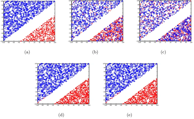
First, we use the synthetic 2D linearly separable data set shown in Figure 1(a). We observe from experiments that our methods achieve over 90% accuracy even whenρ+1 =ρ−1= 0.4.
Figure 1 shows the performance of ˜`logon the data set for different noise rates. Next, we use a
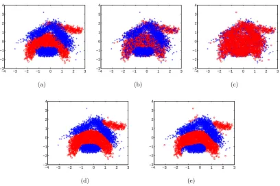
2D UCI benchmark non-separable data set (‘banana’). The data set and classification results using C-SVM (which corresponds to vanilla SVM for uniform noise rates, α∗ = 1/2) are shown in Figure 2. The results for higher noise rates are impressive as observed from Figures 2(d) and 2(e). The ‘banana’ data set has been used in previous research on classification with noisy labels. In particular, the Random Projection classifier (Stempfel and Ralaivola, 2007) that learns a kernel perceptron in the presence of noisy labels achieves about 84% accuracy atρ+1=ρ−1 = 0.3 as observed from our experiments (as well as shown by Stempfel
and Ralaivola, 2007), and the random hyperplane sampling method (Stempfel et al., 2007) gets about the same accuracy at (ρ+1, ρ−1) = (0.2,0.4) (as reported by Stempfel et al.,
2007). Contrast these with C-SVM that achieves about 90% accuracy at ρ+1 =ρ−1 = 0.2
and over 88% accuracy atρ+1=ρ−1= 0.4.
6.2 Comparison with state-of-the-art methods on UCI benchmark data
−100 −80 −60 −40 −20 0 20 40 60 80 100 −100 −80 −60 −40 −20 0 20 40 60 80 100 (a)
−100 −80 −60 −40 −20 0 20 40 60 80 100 −100 −80 −60 −40 −20 0 20 40 60 80 100 (b)
−100 −80 −60 −40 −20 0 20 40 60 80 100 −100 −80 −60 −40 −20 0 20 40 60 80 100 (c)
−100 −80 −60 −40 −20 0 20 40 60 80 100 −100 −80 −60 −40 −20 0 20 40 60 80 100 (d)
−100 −80 −60 −40 −20 0 20 40 60 80 100 −100 −80 −60 −40 −20 0 20 40 60 80 100 (e)
Figure 1: Classification of linearly separable synthetic data set using ˜`log. The noise-free
data is shown in the leftmost panel. Plots (b) and (c) show training data corrupted with noise rates (ρ+1=ρ−1=ρ) 0.2 and 0.4 respectively. Plots (d) and (e) show
the corresponding classification results. The algorithm achieves 98.5% accuracy even at 0.4 noise rate per class. (Best viewed in color).
best performing variants from among the NHERD family of methods proposed by Crammer et al. 2006, 2009; Dredze et al. 2008), and perceptron algorithm with margin (PAM) which was shown to be robust to label noise by Khardon and Wachman (2007). We use seven standard UCI classification data sets listed in Table 1; here, data sets 1 through 6 are preprocessed and made available by Gunnar R¨atsch.1
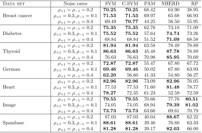
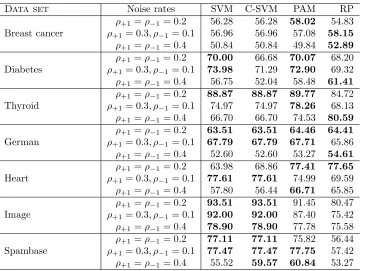
Using linear kernel. Results for the accuracy measure, for different settings of noise rates,
using linear kernel in the compared methods, are shown in Table 2. C-SVM is competitive in 5 out of 7 data sets (Breast cancer, Thyroid, German, Image and Spambase), while relatively poorer in the other two. Note that in many cases, especially whenρ+1=ρ−1, the
standard SVM (i.e. where positive and negative examples are weighted equally) as well as C-SVM (where α parameter that controls the relative weighting is tuned) yield the same accuracy, indicating that the cross-validation effectively selects equal weights; recall that the theory indeed suggests when the noise rates are equal, the optimal choice of weights are equal, i.e. α= 1/2 (see Section 5). The corresponding results for the AM measure, for different settings of noise rates, are shown in Table 5. We find that C-SVM is competitive in three data sets, and NHERD is competitive in most of the data sets. Also observe that
−4 −3 −2 −1 0 1 2 3 −3
−2 −1 0 1 2 3 4
(a)
−4 −3 −2 −1 0 1 2 3
−3 −2 −1 0 1 2 3 4
(b)
−4 −3 −2 −1 0 1 2 3
−3 −2 −1 0 1 2 3 4
(c)
−4 −3 −2 −1 0 1 2 3
−3 −2 −1 0 1 2 3 4
(d)
−4 −3 −2 −1 0 1 2 3
−3 −2 −1 0 1 2 3 4
(e)
Figure 2: Classification of ‘banana’ data set using C-SVM. The noise-free data is shown in (a). Plots (b) and (c) show training data corrupted with noise rates (ρ+1 = ρ−1 =ρ) 0.2 and 0.4 respectively. Note that forρ+1=ρ−1,α∗ = 1/2 (i.e. C-SVM
reduces to regular SVM). Plots (d) and (e) show the corresponding classification results (Accuracies are 90.6% and 88.5% respectively). Even when 40% of the labels are corrupted (ρ+1=ρ−1= 0.4), the algorithm recovers the class structures
as observed from plot (e). Note that the accuracy of the method atρ= 0 is 90.8%.
at high noise rates AM is a more reliable measure of performance — in case of the four data sets Breast cancer, Diabetes, Thyroid and German which have class imbalance, the classifier optimized for the accuracy measure (Table 2) tends to bias its predictions towards the majority class (suggested by accuracy values matching the class imbalance ratio) but the achieved AM values are low.
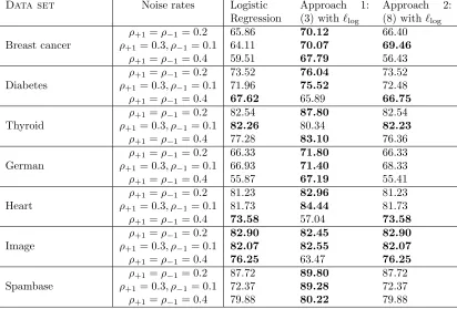
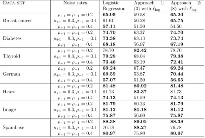
We present the results for logistic loss based methods, using linear kernel, in Tables 3 and 6. As in the case of SVM based methods, we find, when ρ+1 = ρ−1, the standard
logistic regression (i.e. where positive and negative examples are weighted equally) as well as weighted logistic regression in the third column (where α parameter that controls the relative weighting is tuned) yield the same accuracy, indicating that the cross-validation effectively selects equal weights. In terms of accuracy, we find that ˜`log (in the second
Data set Dim Num. Positives Num. Negatives
Breast cancer 9 77 186
Diabetes 8 268 500
Thyroid 5 65 150
German 20 300 700
Heart 13 120 150
Image 18 1188 898
Spambase 57 1813 2788
Table 1: UCI data sets used in experiments.
Data set Noise rates SVM C-SVM PAM NHERD RP
ρ+1=ρ−1= 0.2 70.25 70.25 68.42 64.90 38.95
Breast cancer ρ+1= 0.3, ρ−1= 0.1 71.53 71.53 69.97 65.68 66.93
ρ+1=ρ−1= 0.4 69.49 70.77 44.25 56.50 55.95
ρ+1=ρ−1= 0.2 75.35 75.35 62.76 73.18 71.09
Diabetes ρ+1= 0.3, ρ−1= 0.1 75.52 75.52 57.64 74.74 73.26
ρ+1=ρ−1= 0.4 68.84 68.84 51.52 71.09 68.58
ρ+1=ρ−1= 0.2 81.94 81.94 63.58 78.49 78.89
Thyroid ρ+1= 0.3, ρ−1= 0.1 86.63 86.63 45.48 87.78 78.89
ρ+1=ρ−1= 0.4 76.63 76.63 70.98 85.95 70.69
ρ+1=ρ−1= 0.2 72.87 72.87 55.47 67.80 67.72
German ρ+1= 0.3, ρ−1= 0.1 69.46 69.46 50.02 67.80 63.93
ρ+1=ρ−1= 0.4 62.20 56.60 41.33 54.80 56.27
ρ+1=ρ−1= 0.2 82.96 82.96 73.09 82.96 76.05
Heart ρ+1= 0.3, ρ−1= 0.1 77.53 77.53 71.60 81.48 78.77
ρ+1=ρ−1= 0.4 78.27 72.35 61.23 52.59 72.59
ρ+1=ρ−1= 0.2 79.55 79.55 70.66 77.76 80.51
Image ρ+1= 0.3, ρ−1= 0.1 74.05 74.05 68.94 79.39 81.02
ρ+1=ρ−1= 0.4 73.73 73.73 63.66 69.61 70.79
ρ+1=ρ−1= 0.2 87.03 87.03 40.04 88.67 62.22
Spambase ρ+1= 0.3, ρ−1= 0.1 88.61 88.61 39.46 76.80 63.33
ρ+1=ρ−1= 0.4 81.28 81.28 39.17 82.03 66.00
Table 2: UAcc measure of classification (linear) algorithms on UCI benchmark data sets. Entries
within 1% from the best in each row are in bold. All the methods use linear kernel. All method-specific parameters are estimated through cross-validation. We show the best performing NHERD variant (‘project’ and ‘exact’) in each case.
Using Gaussian kernel. For kernelized algorithms, we set the Gaussian kernel width
parameterγ to 1/dwheredis the dimensionality of data (the default parameter setting in
libsvm). The results comparing SVM based methods are presented in Tables 4 and 7 for accuracy and AM measure respectively. We see a similar trend in performances as in the case of linear kernel. Note that the NHERD method is not kernelizable, so the results are omitted.
Data set Noise rates Logistic Regression
Approach 1: (3) with`log
Approach 2: (8) with`log
ρ+1=ρ−1= 0.2 65.86 70.12 66.40
Breast cancer ρ+1= 0.3, ρ−1= 0.1 64.11 70.07 69.46
ρ+1=ρ−1= 0.4 59.51 67.79 56.43
ρ+1=ρ−1= 0.2 73.52 76.04 73.52
Diabetes ρ+1= 0.3, ρ−1= 0.1 71.96 75.52 72.48
ρ+1=ρ−1= 0.4 67.62 65.89 66.75
ρ+1=ρ−1= 0.2 82.54 87.80 82.54
Thyroid ρ+1= 0.3, ρ−1= 0.1 82.26 80.34 82.23
ρ+1=ρ−1= 0.4 77.28 83.10 76.36
ρ+1=ρ−1= 0.2 66.33 71.80 66.33
German ρ+1= 0.3, ρ−1= 0.1 66.93 71.40 68.33
ρ+1=ρ−1= 0.4 55.87 67.19 55.41
ρ+1=ρ−1= 0.2 81.23 82.96 81.23
Heart ρ+1= 0.3, ρ−1= 0.1 81.73 84.44 81.73
ρ+1=ρ−1= 0.4 73.58 57.04 73.58
ρ+1=ρ−1= 0.2 82.90 82.45 82.90
Image ρ+1= 0.3, ρ−1= 0.1 82.07 82.55 82.07
ρ+1=ρ−1= 0.4 76.25 63.47 76.25
ρ+1=ρ−1= 0.2 87.72 89.80 87.72
Spambase ρ+1= 0.3, ρ−1= 0.1 72.37 89.28 72.37
ρ+1=ρ−1= 0.4 79.88 80.22 79.88
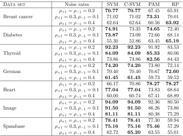
Table 3: UAccmeasure of logistic loss based classification algorithms on UCI benchmark data sets.
Data set Noise rates SVM C-SVM PAM RP ρ+1 =ρ−1= 0.2 70.77 70.77 67.45 65.91
Breast cancer ρ+1= 0.3, ρ−1= 0.1 71.02 71.02 73.31 70.01
ρ+1 =ρ−1= 0.4 62.64 62.64 60.56 63.92
ρ+1 =ρ−1= 0.2 74.91 73.35 74.65 72.40
Diabetes ρ+1= 0.3, ρ−1= 0.1 73.87 73.09 72.66 68.14
ρ+1 =ρ−1= 0.4 55.30 52.86 63.45 65.19
ρ+1 =ρ−1= 0.2 92.23 92.23 91.92 83.53
Thyroid ρ+1= 0.3, ρ−1= 0.1 84.09 84.09 85.33 80.06
ρ+1 =ρ−1= 0.4 73.86 73.86 82.56 84.43
ρ+1 =ρ−1= 0.2 74.20 74.20 73.80 72.14
German ρ+1= 0.3, ρ−1= 0.1 70.40 70.40 70.67 72.60
ρ+1 =ρ−1= 0.4 61.45 61.45 59.73 59.52
ρ+1 =ρ−1= 0.2 66.17 70.86 78.27 78.27
Heart ρ+1= 0.3, ρ−1= 0.1 77.04 77.04 73.83 68.64
ρ+1 =ρ−1= 0.4 60.00 60.74 67.41 68.89
ρ+1 =ρ−1= 0.2 94.09 94.09 92.36 80.50
Image ρ+1= 0.3, ρ−1= 0.1 91.50 91.50 86.26 73.86
ρ+1 =ρ−1= 0.4 81.11 81.11 80.38 75.29
ρ+1 =ρ−1= 0.2 78.41 78.41 77.30 59.94
Spambase ρ+1= 0.3, ρ−1= 0.1 75.16 75.16 75.46 57.29
ρ+1 =ρ−1= 0.4 62.72 65.20 63.55 55.01
Table 4: UAccmeasure of classification (kernelized) algorithms on UCI benchmark data sets. Entries
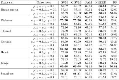
Data set Noise rates SVM C-SVM PAM NHERD RP ρ+1=ρ−1= 0.2 50.82 50.82 62.94 66.14 37.58
Breast cancer ρ+1= 0.3, ρ−1= 0.1 57.48 57.48 59.94 64.28 62.69
ρ+1=ρ−1= 0.4 52.59 50.83 56.52 56.21 56.02
ρ+1=ρ−1= 0.2 70.85 70.85 69.90 74.48 72.17
Diabetes ρ+1= 0.3, ρ−1= 0.1 75.26 75.26 66.19 76.66 73.80
ρ+1=ρ−1= 0.4 63.15 63.15 60.16 71.88 69.00
ρ+1=ρ−1= 0.2 72.16 72.16 67.25 77.67 74.16
Thyroid ρ+1= 0.3, ρ−1= 0.1 79.69 79.69 55.05 83.99 74.05
ρ+1=ρ−1= 0.4 64.23 64.23 55.45 82.97 66.62
ρ+1=ρ−1= 0.2 62.15 62.15 64.68 70.64 67.72
German ρ+1= 0.3, ρ−1= 0.1 69.59 69.59 63.09 70.45 65.23
ρ+1=ρ−1= 0.4 54.13 53.51 54.62 54.70 56.00
ρ+1=ρ−1= 0.2 81.82 81.82 75.05 82.97 75.99
Heart ρ+1= 0.3, ρ−1= 0.1 77.98 77.98 73.10 82.19 78.46
ρ+1=ρ−1= 0.4 76.42 67.81 66.16 52.07 72.85
ρ+1=ρ−1= 0.2 76.43 76.43 67.29 76.75 79.23
Image ρ+1= 0.3, ρ−1= 0.1 75.70 75.70 67.13 80.21 76.87
ρ+1=ρ−1= 0.4 69.68 69.68 58.03 70.64 70.68
ρ+1=ρ−1= 0.2 85.88 85.88 50.00 88.62 61.19
Spambase ρ+1= 0.3, ρ−1= 0.1 88.27 88.27 52.07 80.06 67.67
ρ+1=ρ−1= 0.4 78.81 78.81 50.00 81.51 63.26
Table 5: UAM measure of classification (linear) algorithms on UCI benchmark data sets. Entries
Data set Noise rates Logistic Regression
Approach 1: (3) with`log
Approach 2: (8) with`log
ρ+1=ρ−1= 0.2 65.95 59.58 65.20
Breast cancer ρ+1= 0.3, ρ−1= 0.1 61.61 56.28 65.75
ρ+1=ρ−1= 0.4 57.11 51.50 54.50
ρ+1=ρ−1= 0.2 74.70 63.37 74.70
Diabetes ρ+1= 0.3, ρ−1= 0.1 73.38 63.13 73.74
ρ+1=ρ−1= 0.4 68.18 56.07 67.19
ρ+1=ρ−1= 0.2 78.70 82.42 78.70
Thyroid ρ+1= 0.3, ρ−1= 0.1 79.28 68.04 79.38
ρ+1=ρ−1= 0.4 73.46 53.19 72.41
ρ+1=ρ−1= 0.2 69.24 67.47 69.24
German ρ+1= 0.3, ρ−1= 0.1 69.59 53.87 70.44
ρ+1=ρ−1= 0.4 57.07 51.50 56.65
ρ+1=ρ−1= 0.2 81.48 80.92 81.48
Heart ρ+1= 0.3, ρ−1= 0.1 81.73 83.37 81.73
ρ+1=ρ−1= 0.4 74.13 51.59 74.13
ρ+1=ρ−1= 0.2 81.79 80.23 81.79
Image ρ+1= 0.3, ρ−1= 0.1 81.12 81.18 81.12
ρ+1=ρ−1= 0.4 75.87 56.60 75.87
ρ+1=ρ−1= 0.2 88.38 89.05 88.38
Spambase ρ+1= 0.3, ρ−1= 0.1 76.78 88.27 76.78
ρ+1=ρ−1= 0.4 80.97 75.80 80.97
Table 6: UAM measure of logistic loss based classification algorithms on UCI benchmark data sets.
Data set Noise rates SVM C-SVM PAM RP ρ+1 =ρ−1= 0.2 56.28 56.28 58.02 54.83
Breast cancer ρ+1= 0.3, ρ−1= 0.1 56.96 56.96 57.08 58.15
ρ+1 =ρ−1= 0.4 50.84 50.84 49.84 52.89
ρ+1 =ρ−1= 0.2 70.00 66.68 70.07 68.20
Diabetes ρ+1= 0.3, ρ−1= 0.1 73.98 71.29 72.90 69.32
ρ+1 =ρ−1= 0.4 56.75 52.04 58.48 61.41
ρ+1 =ρ−1= 0.2 88.87 88.87 89.77 84.72
Thyroid ρ+1= 0.3, ρ−1= 0.1 74.97 74.97 78.26 68.13
ρ+1 =ρ−1= 0.4 66.70 66.70 74.53 80.59
ρ+1 =ρ−1= 0.2 63.51 63.51 64.46 64.41
German ρ+1= 0.3, ρ−1= 0.1 67.79 67.79 67.71 65.86
ρ+1 =ρ−1= 0.4 52.60 52.60 53.27 54.61
ρ+1 =ρ−1= 0.2 63.98 68.86 77.41 77.65
Heart ρ+1= 0.3, ρ−1= 0.1 77.61 77.61 74.99 69.59
ρ+1 =ρ−1= 0.4 57.80 56.44 66.71 65.85
ρ+1 =ρ−1= 0.2 93.51 93.51 91.45 80.47
Image ρ+1= 0.3, ρ−1= 0.1 92.00 92.00 87.40 75.42
ρ+1 =ρ−1= 0.4 78.90 78.90 77.78 75.58
ρ+1 =ρ−1= 0.2 77.11 77.11 75.82 56.44
Spambase ρ+1= 0.3, ρ−1= 0.1 77.47 77.47 77.75 57.42
ρ+1 =ρ−1= 0.4 55.52 59.57 60.84 53.27
Table 7: UAM measure of classification (kernelized) algorithms on UCI benchmark data sets.
6.3 Knowledge of noise rates
The proposed algorithms require the knowledge of noise rates ρ+1 and ρ−1. However, in
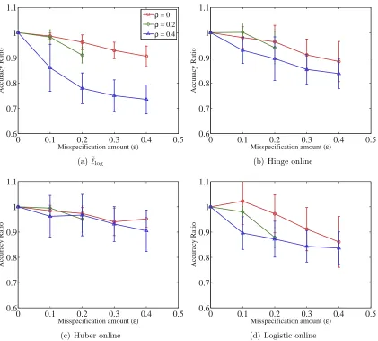
practice, we do not know the true value of noise rates, and therefore we resort to cross-validating the values in our experiments. In some cases (and domains), we may be able to approximately specify noise rates. This motivates our study presented in Figure 3. True noise ratesρ+1=ρ−1 =ρare misspecified as (ρ+1±, ρ−1±) for∈ {0.1,0.2,0.3,0.4}. The
ratio between the average accuracy for a given and the accuracy at= 0, i.e. when true noise rates are specified, is a measure of sensitivity of the algorithms to-misspecification of noise rates. We would want the ratio to be close to 1 for a given, which would suggest that the method is fairly robust with respect to the -misspecification. The results in Figure 3 show that the proposed methods are robust to -misspecification of noise rates, which in turn suggests that our methods can find better use in applications where labels can be noisy and noise rates are approximately known, without resorting to ad-hoc cross-validation procedures on the noisy data. We emphasize here that in case the true noise rates are known, our methods can benefit from that knowledge as observed from our experiments, whereas the competitive methods cannot as they do not involve noise rates.
7. Conclusions and Future Work
We addressed learning in the presence of asymmetric random label noise with respect to gen-eral cost-sensitive utilities. We have obtained gengen-eral theoretical results as well as efficient algorithms for this setting using the methods of unbiased estimators and weighted loss func-tions. The proposed algorithms are easy to implement and the classification performance is encouraging even at high noise rates and in particular is competitive with state-of-the-art methods on benchmark data. Our developments provide a new family of methods that can be applied to the positive-unlabeled learning problem (Elkan and Noto, 2008), but the implications of our methods for this setting should be carefully analyzed. We could consider harder noise models such as label noise depending on the example, and nastier variants of label noise where labels to flip are chosen adversarially.
Our analysis in this paper covers cost-sensitive classification losses, but there are other measures used in practice such as Fβ, that are not covered by our family. Consistent
learning for such general performance measures is beginning to be understood in the noise-free setting (Koyejo et al., 2014; Narasimhan et al., 2014). It would be interesting to see if we can extend some of the ideas in this paper to more general utility measures. It will also be of interest to extend our methods to deal with label noise in more general learning problems such as classification with a reject option, multiclass classification, learning with partial labels, learning to rank, and multilabel classification. Some of these extensions have begun to occur (van Rooyen and Williamson, 2015) but others are yet to be explored.
Acknowledgments
0 0.1 0.2 0.3 0.4 0.5 0.6
0.7 0.8 0.9 1 1.1
Misspecification amount (ε)
Accuracy Ratio
ρ = 0
ρ = 0.2
ρ = 0.4
(a) ˜`log
0 0.1 0.2 0.3 0.4 0.5 0.6
0.7 0.8 0.9 1 1.1
Misspecification amount (ε)
Accuracy Ratio
(b) Hinge online
0 0.1 0.2 0.3 0.4 0.5 0.6
0.7 0.8 0.9 1 1.1
Misspecification amount (ε)
Accuracy Ratio
(c) Huber online
0 0.1 0.2 0.3 0.4 0.5 0.6
0.7 0.8 0.9 1 1.1
Misspecification amount (ε)
Accuracy Ratio
(d) Logistic online
Figure 3: Study of sensitivity of batch (˜`log) and online (Hinge, Huber and Logistic)
meth-ods (Algorithm 1) to specification of noise ratesρ+1 and ρ−1. True noise rates ρ+1 = ρ−1 = ρ are misspecified as (ρ+1±, ρ−1±) for ∈ {0.1,0.2,0.3,0.4}.
The ratio between the average accuracy for a givenand the accuracy at= 0, i.e. when true noise rates are specified, is plotted for different values of noise rates ρ. The ratio is computed for each of the 6 UCI data sets in Table 1 and the mean and the standard deviation of the ratios are shown. Ratio being equal to 1 for a given means that the performance of the algorithm, on average, is unaltered by misspecification of noise rates up to . As expected, the ratio de-creases, i.e. the algorithms perform worse asincreases. Most of the ratios being close to 1 suggests that the proposed methods are fairly robust with respect to
References
D. Angluin and P. Laird. Learning from noisy examples. Mach. Learn., 2(4):343–370, 1988.
Javed A. Aslam and Scott E. Decatur. On the sample complexity of noise-tolerant learning.
Inf. Process. Lett., 57(4):189–195, 1996.
Peter L. Bartlett, Michael I. Jordan, and Jon D. McAuliffe. Convexity, classification, and risk bounds. Journal of the American Statistical Association, 101(473):138–156, 2006.
Shai Ben-David, D´avid P´al, and Shai Shalev-Shwartz. Agnostic online learning. In
Confer-ence on Learning Theory (COLT), 2009.
Battista Biggio, Blaine Nelson, and Pavel Laskov. Support vector machines under adver-sarial label noise. J. Mach. Learn. Res. (JMLR), 20:97–112, 2011.
Gilles Blanchard and Clayton Scott. Decontamination of mutually contaminated models.
In International Conference on Artificial Intelligence and Statistics (AISTATS), pages
1–9, 2014.
A. Blum and T. Mitchell. Combining labeled and unlabeled data with co-training. In
Computational Learning Theory (COLT), pages 92–100. ACM, 1998.
Tom Bylander. Learning linear threshold functions in the presence of classification noise.
In Conference on Learning Theory (COLT), pages 340–347, NY, USA, 1994. ACM.
Tom Bylander. Learning noisy linear threshold functions. Technical Report, 1998.
Nicol`o Cesa-Bianchi, Eli Dichterman, Paul Fischer, Eli Shamir, and Hans Ulrich Simon. Sample-efficient strategies for learning in the presence of noise. J. ACM, 46(5):684–719, 1999.
Nicol`o Cesa-Bianchi, Shai Shalev-Shwartz, and Ohad Shamir. Online learning of noisy data.
IEEE Transactions on Information Theory, 57(12):7907–7931, 2011.
Edith Cohen. Learning noisy perceptrons by a perceptron in polynomial time. In
Founda-tions of Computer Science, pages 514–523. IEEE, 1997.
K. Crammer and D. Lee. Learning via Gaussian Herding. InNeural Information Processing
Systems (NIPS), pages 451–459, 2010.
Koby Crammer, Ofer Dekel, Joseph Keshet, Shai Shalev-Shwartz, and Yoram Singer. Online passive-aggressive algorithms. J. Mach. Learn. Res. (JMLR), 7:551–585, 2006.
Koby Crammer, Alex Kulesza, and Mark Dredze. Adaptive regularization of weight vectors.
In Neural Information Processing Systems (NIPS), pages 414–422, 2009.
Mark Dredze, Koby Crammer, and Fernando Pereira. Confidence-weighted linear classifi-cation. In International Conference on Machine Learning (ICML), pages 264–271, 2008.
C. Elkan and K. Noto. Learning classifiers from only positive and unlabeled data. In Intl.