Performance Comparison of A New Non-RSSI Based Wireless Transmission Power Control Protocol with RSSI Based Methods:Experimentation with Real World Data

(1)

Performance Comparison of A New Non-RSSI Based Wireless

Transmission Power Control Protocol with RSSI Based Methods:

Experimentation with Real World Data

Debraj Basu

*

, Gourab Sen Gupta, Giovanni Moretti, Xiang Gui

School of Engineering and Advanced Technology, Massey University, New Zealand

Received 13 August 2015; received in revised form 03 November 2015; accepted 11 December 2015

Abstract

In this paper, simulations with MATLAB are used to compare the performance of a RSSI-based output power control with non-RSSI based adaptive power in terms of saving energy and extending the lifetime of battery powered wireless sensor nodes. This non-RSSI (received signal strength indicator) based adaptive power control algorithm does not use RSSI side information to estimate the link quality. The non-RSSI based approach has a unique methodology to choose the appropriate power level. It has drop-off algorithm that enables it to come back from a higher to a lower power level when deemed necessary. The performance parameters are compared with the RSSI-based adaptive power control algorithm and fixed power transmission. In order to evaluate the protocols in the real world scenarios, RSSI data from different indoor radio environments are collected. In simulation, these RSSI values are used as an input to the RSSI based power control algorithm to calculate the packet success rates and the energy expenditures. In this paper we present extensive analysis of the simulation results to find out the advantages and limitations of the non-RSSI based adaptive power control algorithm under different channel conditions.

Keywords: wireless sensor network, energy consumption optimization, adaptive power control

1. Introduction

The proliferation of low power wireless sensor networks and their discreet presence have introduced a new paradigm in data collection and analysis of target parameters in both indoor and outdoor environments. This has been differently named in the literature and the industry, like ‘invisible”, “pervasive” or “ubiquitous” [1] computing. Others prefer to refer to it as “ambient intelligence” [2]. The broad idea is that there will be sensors that are able to exchange information with a certain base station or hub and perform an assigned task. The sensors, the computational and the communication units, along with the hub, form the ubiquitous sensor network (USN). The term ubiquitous is applied to the collection and utilization of information in real time, at any-time and any-where. The technology has enormous potential and a wide range of applications such as, environmental monitoring, health monitoring for assisted living (smart home environments) and industrial and plant monitoring (Industrial automation).

1.1 Related work in transmission power control for energy efficiency

Power saving approaches can be broadly classified into media access control (MAC) layer solutions and network layer

(2)

solutions [3]. Network layer solution means that the different transmission parameters can be modified to achieve the set goal. This paper discusses the use of received link quality information (RSSI/LQI) to adjust output transmission power.

1.2 RSSI/LQI based power control algorithms for energy efficiency

The RSSI-based power control approaches is guided by closed loop control between the transmitting node and the receiving base station mechanism. RSSI is a measurement of signal power and which is averaged over 8 symbols of each incoming packet [4]. On the other hand, LQI is usually vendor specific and is measured based on the first eight symbols of the received packet as a score between 50 and 100 [5].The general steps are described below as

• The transmitter sends packet at an updated power level to the receiver

• Receiver measures the RSSI

• If the RSSI is below the threshold that is required for faithful packet delivery, then the receiver sends the control packet with the new transmission power level.

• At the transmitter, the control packet is received and the current power level is updated for packet delivery

During initialization phase, the transmitter needs to know the power level at which it should transmit to successfully deliver the packet. In this phase, the transmitter sends several packets at all its available power levels. In return, it receives RSSI values for each power levels. Based on the mapping of the RSSI and the output power level, the transmitter selects the required power level.

In paper [4], Shan Lin et al. have introduced adaptive transmission power control (ATPC) that maintains a neighbor table at each node and a feedback loop for transmission power control between each pair of nodes. ATPC provided the first dynamic transmission power algorithm for WSN that uses all the available power output levels of CC2420 [6].

Practical-TPC [7] is a receiver oriented protocol that is considered robust in dynamic wireless environments and uses packet reception rate (PRR) values to compute the transmission power that should be used by the sender in the next attempt. While ATPC uses all 32 power levels, there are some algorithms that divide these 32 power levels into 8 levels, as in [3]. The work described is this paper aims to avoid the need for such probe packets and their associated energy cost. ART (Adaptive and Robust Topology control) protocol [8] has been designed for complex and dynamic radio environments. It adapts the transmission power in response to variation in link quality or degree of contention. Analysis of the paper has suggested that RSSI and LQI (Link Quality Indicator) may not be good or the most reliable indicators of link quality, especially in robust indoor radio environment.

Paper [3] also has an initialization phase and a maintenance phase while adjusting transmission power. In the initialization phase, each of the sensor nodes uses the 8 power levels of CC2420 to send 100 probe packets in each of the power levels. It sets the packet delivery ratio (PDR) threshold to 80% instead of the RSSI threshold to determine the minimum power level with which the nodes must communicate with each other. In the maintenance phase, the aim is to adjust the transmission power level with the changing environment.

(3)

The data recovery actions have three options to choose from. They are

• Use of error correction code to recover the original data packet at the receiver

• Retransmit when the error correction mechanism has failed due to severe distortion

• Drop some packets to save energy for transmission of higher priority packets

In [10], the approach is similar to ATPC where the power-distance table is maintained at each node. The distance is the minimum power of one node with the neighboring node. In multi-hop wireless sensor network, optimization of the transmission power is, therefore, the shortest path problem based on the power-distance relationship. In [11], the authors have proposed a power control algorithm in which each sensor node also uses beacon messages to determine its neighbors and the corresponding minimum transmission power. After the neighbors are discovered, the adaptive algorithm finds the optimal power so that it is able to meet its target of communicating with a given number of neighboring nodes. Authors have combined dynamic transmission power control of the link layer protocol with the reduction of duty cycle of MAC layer to save energy.

Paper [12] has introduced the term “link inefficiency” while characterizing the link quality metrics of energy constrained wireless sensor nodes. Link inefficiency is defined as the inverse of the packet success probability as it represents the mean number of transmissions for a successful transmission at a given time. The expected energy consumption is, therefore, proportional to the link inefficiency. This paper proposes the time average energy consumption as the cost metrics.

The application of an adaptive power control algorithm for IEEE 802.11 in the technical report of [13] aims to modulate the transmit power based on the distance between the communicating nodes to the minimum level such that the destination node still achieves correct reception of a packet despite intervening path loss and fading. It used a radio module with configurable output power level (0 to 25 dBm). The receiver only sends the control packet containing the optimal transmission power level when there are significant changes in the RSSI values.

RSSI/LQI based adaptive power control algorithms are an attractive alternative to save energy. It is to be noted that these algorithms are mainly designed for multi-hop network where each sensor node broadcast beacon packets and discover its neighbor to which it can transmit at minimum power. However, there are two factors that are worth considering. They are

• There is an initial overhead cost for building up the RSSI vs. Power level table.

• In case the sensor is mobile, the refreshing frequency of the table becomes crucial and that also adds up to the cost.

• Even when the sensors are stationary, there is no clear indication in any of the papers ([3-4], [6-13]) as to what would be the ideal channel sampling frequency that would optimise energy efficiency.

(4)

Table 1 Operational modes and current consumptions of NRF24L01+ Operational mode Current consumed mA Transmission @ 0 dBm output power (MIN) 11.3

Transmission @ -6 dBm output power (LOW) 9 Transmission @ -12 dBm output power (HIGH) 7.5 Transmission @ -18 dBm output power (MAX) 7

The transceiver can transmit at four power levels: -18 dBm, -12 dBm, -6 dBm and 0 dBm. In general, a wireless transceiver has different modes of operation.

Among other methods of energy aware data transmission in WSN or mobile application, the work of Zhang et.al has been noteworthy. In [15], the authors have proposed a novel topology control approach for wireless sensor networks (WSNs) where the edge weight and vertex strength take sensor energy, transmission distance, and flow into consideration. Zhang and Liang have proposed a novel method of service aware computing for uncertain mobile applications to ensure QoS for these devices supporting various applications [16]. In industrial applications of WSNs, an energy-balanced routing method based on forward-aware factor (FAF-EBRM) has been proposed by the authors in [17]. In this multi-hop routing algorithm, the next node is selected based on information about the link weight and forward energy density. In [18], authors have designed and implemented a solution of embedded un-interruptible power supply (UPS) system forward for long-distance monitoring and controlling of UPS based on Web. Zhang et.al, have proposed a novel multicast routing method with minimum transmission for WSN of cloud computing service [19].

In [20], Zhang has proposed a fusion decision method to support an attentive mobile learning paradigm. The learning method tracks the users’ movement without any active devices. The objective is to achieve seamless mobility for mobile services, especially mobile web-based learning. In the RFID (radio-frequency identification) domain, one of the key issues is the packet losses due to collision when the RFID tags transmit within the collision window (time). In [21], a novel anti-collision approach has been proposed by Zhang et.al. In this method, a mapped correlation of the IDs of the RFID tags is used to increase the association between the tags. In [22], the authors have proposed agent-based proactive migrating method with service discovery and key frames selection strategy. The designed system is convenient to work and use during mobility, and which is useful for mobile user in the big data environments (BDE).

2. Adaptive transmission power control methods: Non-RSSI based and RSSI-based

This section discusses about the novel transmission power control protocol that does not use RSSI data for channel estimation and the RSSI-based power control method.

2.1 Non- RSSI/LQI based channel estimation and power control algorithms for energy efficiency

(5)

drop-off. Fig. 1 shows the state transition diagram of the adaptive power control algorithm. State transition occurs depending on the power level at which the transmission is successful or has failed.

Fig. 1 State transition diagram of the adaptive algorithm

The objective of the adaptive power control algorithm is to respond to the packet error rate and move to a new state with different retry limits. The adaptive algorithm is designed in such a way that it takes into account the performance in each state. Each state has a different retry limit. Increasing state number indicates poorer channel quality. The proposed adaptive algorithm does not allow retransmission in the same power level except when it is in state 4 and transmitting at 0 dBm. When the system is in state 4, it is considered the worst channel condition and three retries are allowed. The retry limit of state 1 is three. However, the retry limit of states 2 and 3 have been set at 2 and 1. The asymmetry is because the increase in the retry limit in states 2 and 3 can increase the current consumption while only marginally improving the packet success rate.

Table 2 shows the available power levels based on the states. Transmission starts at the lowest available power level of that particular state. The transmitter can be in any one of the states during the start of transmission of a packet. There are two separate algorithms that determine the state transitions, one from a lower state to higher state and the other from a higher to lower states. The logic to transit to lower states also includes situations when it remains in the same state or transit to a lower state.

Table 2 States, power levels, and retry limits

State 1 2 3 4

Av

ailab

le

p

o

wer

lev

els Minimum (M)

Low (L) Low (L)

High (H) High (H) High (H)

Maximum (X) Maximum (X) Maximum (X) Maximum (X)

Number of retries 3 2 1 3

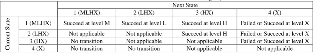
Table 3 describes the state transition matrix when state level goes up. All the state transition decisions depend on the success or failure of the packet being transmitted to the destination hub.

Table 3 State transition matrix when state levels go up Next State

1 (MLHX) 2 (LHX) 3 (HX) 4 (X)

C

u

rr

en

t State

1 (MLHX) Succeed at level M Succeed at level L Succeed at level H Failed or Succeed at level X 2 (LHX) Not applicable Not applicable Succeed at level H Failed or Succeed at level X 3 (HX) No transition Not applicable Not applicable Failed or Succeed at level X

(6)

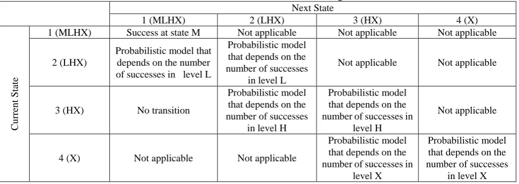
Table 4 State transition matrix when state levels go down Next State

1 (MLHX) 2 (LHX) 3 (HX) 4 (X)

C

u

rr

en

t State

1 (MLHX) Success at state M Not applicable Not applicable Not applicable

2 (LHX)

Probabilistic model that depends on the number of successes in level L

Probabilistic model that depends on the number of successes

in level L

Not applicable Not applicable

3 (HX) No transition

in level H

Probabilistic model that depends on the number of successes in

level H

Not applicable

4 (X) Not applicable Not applicable

Probabilistic model that depends on the number of successes in

level X

in level X Table 4 describes the state transition logic when state level goes down. The primary objective of the adaptive algorithm is to save energy by transmitting at a power level that is enough to send the packet successfully through the channel. For example, when the system is in state 4, it is transmitting at the maximum power. With time, the channel condition can improve and packet can be successfully transmitted at a lower power level. If the system drops down to state 3, the transmission starts at a lower power level. This drop-off from a higher state to a lower state is determined by a drop-off algorithm which is probabilistic in nature.

In the proposed adaptive algorithm, the drop-off or the back-off process is dependent on the number of successes (S) in the higher power level and a drop-off factor (R). By default, the drop-off factor is 1. The probability of the system to drop-off to a lower power level is represented by Equation (1).

P(drop-off)=1- e(-RS) (1)

Here, Pdrop-off = probability of drop-off

S = the number of successes in that power level of the higher state R = drop-off factor

(7)

The plots in Fig. 2 show the state transition probability based on different values of R. When there is a state change, the value of S is reset to 0. Overall, the value of R indicates as to how fast the system will fall from a higher state to a lower state. When there is no success, the probability of state transition is 0, meaning that there will be no state transition. At the same time, when the number of successes is too high, it converges to 0.

Back-off algorithms are extensively used in data communication (both wired and wireless) by MAC protocols to resolve contention among transmitting nodes to acquire channel access. In a MAC protocol, the back-off algorithm chooses a random value from the range [0, CW], where CW is the contention window size. The contention window is usually represented in terms of time slots.

The number of time slots to delay before the nth retransmission attempt is chosen as a uniformly distributed random integer r in the range 0 < r < 2k.

where k = min(n, 10), 10 is the maximum number of retries allowed.

The nth retransmission attempt also means that there have been n collisions. For example, after the first collision, it has to retransmit. Based on the back-off algorithm, the sender will choose between 0 and one time slot for the retransmission. After the second collision, the sender will wait anywhere from 0 to three time slots (inclusive). After the third collision, the senders will wait anywhere from 0 to seven time slots (inclusive), and so forth. As the number of retransmission attempts increases, the number of possibilities for delay increases exponentially [25-26].

Similarly, an exponential operator is used in this novel adaptive algorithm to decide to switch from a higher state to a lower state. The drop-off algorithm is dynamic as it re-evaluates at every successful transmission. It gets reset to 0 when it leaves the state and jumps to a lower state and starts a new packet transmission at a lower power level.

In this paper, this protocol is compared with the standard RSSI-based channel estimation and power control algorithm (ATPC) using real world RSSI data when sensors are stationary. The next section explains the ATPC protocol in details.

2.2 ATPC: Adaptive Transmission Power Control for wireless sensor networks

The first adaptive power control protocol for wireless sensor network was proposed in [4]. Results show that the ATPC only consumes 53% of the transmission energy of the maximum transmission power solutions and 78.8 % of that of network level transmission power solutions [3]. In ATPC, the sensor nodes build a model for each of its neighboring nodes that describe the correlation between the transmission power and the link quality. The radio link quality varies over time and with environment. The objective of the ATPC protocol is to find out the minimum transmission power level to maintain a good quality link (~PSR > 98%) and dynamically change the transmission power level over time to address the time varying nature of the wireless channel. Each node sends beacon packets at different transmission power level to the neighboring node and makes note of the RSSI value that it receives on the feedback path. Based on this information, the node builds a predictive model and uses least square approximation method to calculate the desired transmission power level.

(8)

number of sample packets in the setup phase. Based on the empirical findings regarding the temporal variation of the link quality, the paper suggested that one packet per hour would maintain the freshness of the predictive model.

3. Simulation parameters

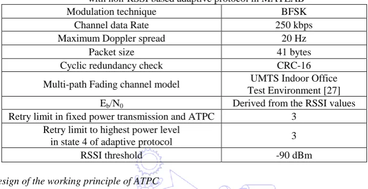
The general simulation parameters are presented in Table 5.

Table 5 General simulation parameters for comparison of ATPC with non-RSSI based adaptive protocol in MATLAB

Modulation technique BFSK

Channel data Rate 250 kbps

Maximum Doppler spread 20 Hz

Packet size 41 bytes

Cyclic redundancy check CRC-16

Multi-path Fading channel model UMTS Indoor Office Test Environment [27]

Eb/N0 Derived from the RSSI values

Retry limit in fixed power transmission and ATPC 3 Retry limit to highest power level

in state 4 of adaptive protocol 3

RSSI threshold -90 dBm

3.1 Simulation design of the working principle of ATPC

The ATPC protocol changes its output power based on the RSSI value of the most recent transmitted packet. It has the four power levels to choose from and uses the decision matrix as explained in Table 6. It is known that the minimum RSSI level to maintain high PSR (> 95%) is approximately -90 dBm [28] [5]. Therefore, it is set as the minimum threshold. Here RSSI_TH is the RSSI threshold and RSSI is the received signal strength indicator of the transmitter packet. In this simulation, the performances of the ATPC are observed at channel sampling/scanning interval of 1, 5, 10, 50 and 100 transmissions.

Table 6 Decision matrix table of ATPC on run time New transmission power level

-18 dBm -12 dBm -6 dBm 0 dBm

C u rr en t Po wer lev

el -18 dBm _{RSSI_TH}RSSI >= RSSI_TH - RSSI <= 6 dB 6 dB < RSSI_TH - RSSI _{< 12 dB} RSSI_TH - RSSI _{> 18dB}

-12 dBm RSSI - RSSI_TH

>= 6 RSSI - RSSI_TH ~ 0 RSSI_TH - RSSI <=6

RSSI_TH - RSSI > 6 -6 dBm RSSI- RSSI_TH

>= 12 dB RSSI- RSSI_TH <=6 dB RSSI - RSSI_TH ~ 0

RSSI-TH- RSSI > = 6 dB 0 dBm RSSI- RSSI_TH

>= 18 dB

6 dB < RSSI – RSSI_TH <= 12 dB

RSSI – RSSI_TH <= 6 dB

RSSI - RSSI_TH ~ 0 During each cycle of power control, the ATPC compares the present RSSI with the RSSI_TH. If the difference between the current RSSI and RSSI_TH is negligible or equal to 0, then the new power level is same as the old power level. These conditions are highlighted in bold brown. Only when the current power level is -18 dBm and RSSI is greater than the RSSI_TH, it sticks to -18 dBm.

3.2 Conditions when to ramp up output power:

 When RSSI_TH > RSSI, it is required to ramp up power for subsequent packets.

(9)

 When 6 dB < RSSI_TH - RSSI < 12 dB, then the output power level is incremented by 12 dB. For example, if the current output power is -18 dBm, then new power level will be -6 dBm. These conditions are highlighted in bold black.

 When RSSI_TH - RSSI ≥ 12 dB and the current power level is -18 dBm, then the new power level will be 0 dBm.  When RSSI_TH - RSSI ≥ 6 dB and the current power level is -12 dBm, then the new power level will be 0 dBm.

3.3 Conditions when to ramp down output power:

 When RSSI - RSSI_TH ≥ 18 dB and output power is 0 dBm, then power level can be decremented by 18 dB to -18 dBm as that will satisfy RSSI ≥ RSSI_TH.

 But when 6 dB < RSSI – RSSI_TH ≤ 12 dB, the output power level decrements to -12 dBm. When RSSI – RSSI_TH ≤ 6 dB, the output power level decrements by 6 dB.

 When RSSI - RSSI_TH ≥ 6 dB and current power level is -12 dBm, then the current power level can be decremented by 6 dB to -18 dBm.

 Finally, when the current power level is -6 dBm and RSSI- RSSI_TH ≤ 6 dB, the power level decrements to -12 dBm, while if RSSI- RSSI_TH ≥ 12 dB, it decrements by 12 dB.

It is known that the minimum RSSI level to maintain high PSR (> 95%) is -90 dBm. Therefore, -90 dBm is set as the minimum threshold. Here RSSI_TH is the RSSI threshold and RSSI is the received signal strength indicator of the transmitter packet. In this simulation, the performances of the ATPC are observed at channel sampling/scanning interval of 1, 5, 10, 50 and 100 transmissions.

4. Performance parameters

The performance parameters are:

• Average cost per successful transmission

• Expected success rate or protocol efficiency [15]

One of the parameters for the optimization is the energy consumed per useful bit transmitted over a wireless link [3, 29]. Similarly in this paper, the cost per successful transmission has been considered.

_

T s avg

S L

C C

P P



 (1)

where

Cs_avg = average energy cost per successful transmission

CT = total cost of transmission

PL = number of lost packets

PS = Number of packets to send

All cost values are measured in mJoules. The total cost of transmission includes the expenditure for the first transmission attempt of a packet and the subsequent retries if the first attempt fails. The total packet to send count does not include the retry packets. Therefore, the denominator in equation 3 is only the count of successfully transmitted packets.

The expected success rate or efficiency is defined as the expected number of successes and takes into account the average number of retries [3]. It can also be defined as the expected number of successes per 100 transmissions. Mathematically,

S L rat e

S T

P P

Succ

P Ret

 

(10)

where

Succrate = expected success rate

RetT = total number of retries

Here PS – PL = total number of successes (Psucc). If both the numerator and denominator are divided by Ps, then in

percentage term, (%) 1 rate avg PSR Succ Ret   (3) where

Retavg = average number of retries per packet and is defined as

T avg S Ret Ret P  ₍₄₎ Here,

1 0 0 succ

S P PSR

P

  ₍₅₎

This parameter indicates the total number of transmissions (on average) to achieve a given packet success rate (PSR).

5. Collection of the RSSI values

In this paper, we have considered a star topology where all the sensors connect to one base station via a single hop. These sensors are responsible for transmitting, for example, temperature, humidity and occupancy data as well as health related vital information in a smart home environment with assisted living. In industrial set up, these sensors transmit key monitoring parameters like humidity and temperature, valve control position among others. These kind of indoor radio environments pose challenge in terms of reliable data delivery and energy efficiency of the sensor node. This is because the radio signal in indoor environment suffers from fading because of multipath propagation where the radio signal from the transmitter arrives at the receiver through multiple paths.

During the busy hour, there are lots of movement of people in between the hub and the transmitting sensor. These movements induce a time varying Doppler shift on multipath components. Fading effect due to frequency shift of the radio signal cannot be ignored when the sensor is stationary. Besides, there can be temporary signal attenuation if people have gathered around. All these affect the radio link quality over time. During the non-busy hours of the University, fading effect due to movement is minimal while the multipath effect still exists. In order to study the variation of the signal level in these kind of indoor radio environment, the RSSI values from the access points of wireless LAN setup in office environment, commercial setup ( shopping center) and social setup (University dining hall) are collected.

The primary source of noise or interference to the signal that is considered in this paper is the signal attenuation because of distance, the partitions in between the transmitter and the base station and the momentary signal fluctuation due to multipath fading as well as movements of people in between the sensor and the base station.

(11)

several APs that were transmitting the radio beacon signal. For the simulation purpose, the RSSI data of that AP was used that was providing the strongest signal. The access point emulates the transmitting sensor while the data collection device (the laptop in this case) acts as the base station.

In simulation, these RSSI values correspond to the minimum output power level (-18 dBm). Hence, it indicates the base channel condition over which power ramping may be required to meet the link quality requirement. This link quality change can be transient or have an effect over a longer period of time. Therefore, the RSSI values can be used to adapt or manipulate the output power. This setup emulates the real world approach of ATPC protocol where the RSSI values from the neighboring node in response to the beacon signal are used to setup the output power level in the initialization phase or during run time. In the single hop topology, it is the hub that piggybacks the RSSI information to the sensor. A 5 second interval between fresh RSSI values indicates that the sensor is transmitting at a rate of 1 packet every 5 seconds and therefore has received the RSSI value as the feedback from the hub.

5.1 Data collection scenarios and calculation of the Eb/N0

There are two types of RSSI variation scenarios that are investigated. They are collected from three different environments after an interval of 5 seconds. They are

 Three sets of long term data over a period of approximately 10 hours from within University campus building. The distance between the transmitter and receiver is approximately 24 meters.

 Three sets of short term data over the busy period of the day (approximately between 90 minutes and 120 minutes) from town shopping centre. The distance between the transmitter and receiver is approximately 30 meters.

 Three set of short term data over the busy period of the day (approximately between 90 minutes and 120 minutes) from University dining hall. The distance between the transmitter and receiver is approximately 25 meters.

5.2 Images of the mentioned scenarios are added in appendix

RSSI is a measurement of signal power and which is averaged over 8 symbols of each incoming packet [4]. The value of RSSI is dependent on the received power, the channel data rate and the noise spectral density (N¬0). If the received average bit energy is denoted by Eb and channel data rate as R, then by definition, in dBm,

0

b E

RSSI Noi s e Power N

  (6)

If the noise floor is assumed to be constant, the RSSI value will depend on the average bit energy and channel data rate. In dBm scale, the relationship between the RSSI and Eb/N0 is linear with intercept of -119.9978 dBm at x-axis. Different data rate

will have different intercept values when the noise floor level is kept constant. The value of -119.9978 is derived from the value of N0 and channel data rate set at 250 kbps for simulation.

Noise PowerKTR (7)

where

K = Boltzmann’s constant (1.28 x10-23 Joules/Kelvin)

(12)

Therefore, the linear relationship between RSSI and Eb/N0 takes the following form in equation (9) which is derived from

equation (7).

0

119.9978 b

E RSSI

N

  (8)

6. Comparison of the optimal cost values of ATPC, adaptive power control and fixed power

transmission using RSSIdata from three different locations

In section 6, performance parameters of ATPC, fixed power and non-RSSI based adaptive power control algorithms are compared.

6.1 Long term RSSI data collected over a period of approximately 10 hours inside University building

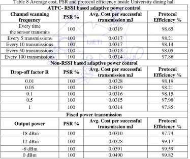
Two sets of data are collected during the period of approximately 10 hours. The busy hour RSSI variation was captured by logging the data between 8:30 a.m. till 5 p.m. The variation of Eb/N0 over time for one of the data sets is presented in Fig. 3. The

RSSI data are collected using a laptop. Using equation (4), the RSSI values are converted to corresponding Eb/N0 values. The

occasional drop to 20 dB is due to fading. Overall, this indicates that the channel link quality is very good.

Fig. 3 The variation of the average Eb/N0 over time. Along x-axis, the numbers of transmissions are noted. The average

Eb/N0 is quite high (>60 dB) and occasionally dropped to 20 dB. Since the distance between the access point and

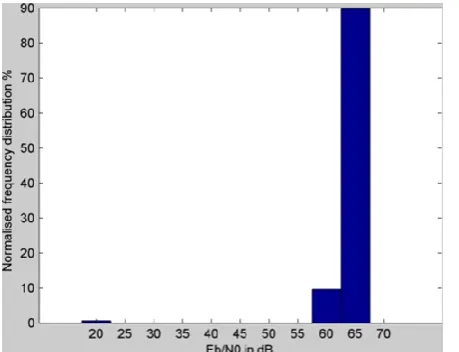
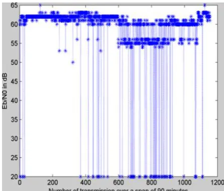
the laptop is constant, the drop in the value is attributed to human movements in between and multipath effects The normalized frequency distribution plots of the Eb/N0 of one of the data sets are shown in Fig. 4.

Fig. 4 The frequency distribution plot of the received Eb/N0 from data set 1 shows that occasionally the signal level

(13)

The normalized frequency distributions of the other two data sets are also similar to the one shown in Fig. 4. The frequency distribution plots also signify the amount of time (%) the channel link quality has remained above a certain value. In both these figures, a high % of time (>85%) the Eb/N0 is more than or equal to 60 dB. The PSR and the efficiency values of all the

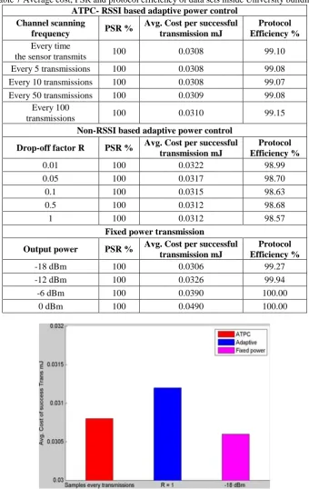
transmission strategies are 100 and higher that 98% respectively and their differences are negligible. Therefore, they are not plotted. Table 7 shows the average values of the performance parameters of the different transmission strategies that are compared in this paper.

Table 7 Average cost, PSR and protocol efficiency of data sets inside University building ATPC- RSSI based adaptive power control

Channel scanning

frequency PSR %

Avg. Cost per successful transmission mJ

Protocol Efficiency % Every time

the sensor transmits 100 0.0308 99.10

Every 5 transmissions 100 0.0308 99.08

Every 100

transmissions 100 0.0310 99.15

Non-RSSI based adaptive power control

Drop-off factor R PSR % Avg. Cost per successful transmission mJ

Protocol Efficiency %

0.01 100 0.0322 98.99

0.05 100 0.0317 98.70

0.1 100 0.0315 98.63

0.5 100 0.0312 98.68

1 100 0.0312 98.57

Fixed power transmission

Output power PSR % Avg. Cost per successful transmission mJ

-18 dBm 100 0.0306 99.27

-12 dBm 100 0.0326 99.94

-6 dBm 100 0.0390 100.00

0 dBm 100 0.0490 100.00

Fig. 5 University building- Comparison of the minimum cost due to different transmission strategy shows that there is hardly any difference in the average cost per successful transmission

(14)

The optimal cost values of each transmission strategy are plotted. The average Eb/N0 values due to transmission at lowest

power level (-18 dBm) is high. That explains the facts from Fig. 5 that fixed power transmission at -18 dBm provides the most energy efficient solution. Any ramping-up in power level will always be wastage of power. The energy consumption values of the adaptive algorithm matches closely when the value of drop-off rate is 0.5. It signifies that the state-based system can perform most energy efficiently under very good link quality when it drops-off the fastest. Section 6.2 compares the energy cost due to ATPC, adaptive power control and fixed power transmission when the RSSI data are collected over a short and busy period of the day.

6.2 Short term busy hour RSSI data collected from University dining hall during busy hours

The variation of the Eb/N0 and their normalized cumulative distribution are plotted in Fig. 6 and Fig. 7. The channel link

quality is still good, with occasional drop to 20 dB due to multi-path fading effect. Since the over-all link quality is still very good (average Eb/N0 > 55 dB), the PSR and the efficiency values in all these cases are 100 and higher than 98% respectively and

their differences are negligible. Therefore, they are not plotted. The tabulated data of the performance parameters averaged over the three sets of observations are presented in table 8. Fig. 8 compares the minimum cost per successful transmission when University dining hall data are used. The difference in the cost is negligible. This is due to the very good quality of link quality (average Eb/N0 >55 dB) for most of the time (> 93%).

Table 8 Average cost, PSR and protocol efficiency inside University dining hall ATPC- RSSI based adaptive power control

the sensor transmits 100 0.0319 98.65

0.01 100 0.0328 98.19

0.05 100 0.0319 98.21

0.1 100 0.0316 98.15

0.5 100 0.0315 97.98

1 100 0.0314 97.85

Output power PSR % Avg. Cost per successful

transmission mJ

-18 dBm 100 0.0310 97.74

-12 dBm 100 0.0328 99.17

-6 dBm 100 0.0391 99.59

(15)

Fig. 6 The variation of the average Eb/N0 from University dining hall during busy hour between 11:30 a.m. and 1:00

p.m. The average Eb/N0 is quite high (>55 dB) and occasionally dropped to 20 dB. The busy hour period shows

that the average Eb/N0 can widely fluctuate between high Eb/N0 (> 55 dB) and low Eb/N0 (~20 dB)

Fig. 7 The frequency distribution plot of the received Eb/N0 from University dining hall during busy hour shows the

rapid fluctuation in the signal level caused by movements of people in between the transmitting sensor and receiver

(16)

6.3 Short term RSSI data collected from town shopping center during busy hours of weekends

Three sets of short time data during busy hours of the town shopping center have been collected. The nature and the distribution of the variation of the Eb/N0 values of the two data sets are almost similar. Therefore, the results of one of the sets are

only presented. The variation of the Eb/N0 is plotted in Fig. 9. It shows the significant variation of link quality during busy hours,

primarily due to multipath fading effect as people move around in the shopping center.

Fig. 9 It shows the variation of the average Eb/N0 from town shopping center during busy hours

between 11:30 a.m. and 1:30 p.m.

The distributions of the Eb/N0 of the three sets of data are similar in nature. Fig. 1 shows the normalized distribution plot.

It is expected that in a town shopping center during busy hours, the signal level will drop more frequently.

Fig. 10 The distribution plot of the received Eb/N0 from town shopping centre during busy

hours between 11:30 a.m. and 1:30 p.m. shows that Eb/N0 at 20 dB is significantly

(17)

Table 9 presents the average values the performance parameters based on the three sets of collected data.

Table 9 Average cost, PSR and protocol efficiency inside shopping centre ATPC- RSSI based adaptive power control

Channel scanning frequency

Avg. Cost per successful

transmission mJ PSR %

the sensor transmits 0.0315 100 98.44

Every 5 transmissions 0.0314 100 98.03

Every 100

transmissions 0.0311 100 97.88

Drop-off factor R Avg. Cost per successful

0.01 0.0328 100 98.19

0.05 0.0319 100 98.11

0.1 0.0316 100 98.12

0.5 0.0300 100 97.90

1 0.0301 100 97.74

Output power Avg. Cost per successful

-18 dBm 0.0310 100 97.91

-12 dBm 0.0327 100 99.24

-6 dBm 0.0391 100 99.67

0 dBm 0.0490 100 99.82

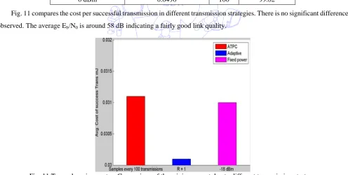
Fig. 11 compares the cost per successful transmission in different transmission strategies. There is no significant difference observed. The average Eb/N0 is around 58 dB indicating a fairly good link quality.

Fig. 11 Town shopping center- Comparison of the minimum cost due to different transmission strategy shows that there is no significant difference in the cost per successful transmission

It can be seen that when the average Eb/N0 is high (> 55 dB), then even momentary fluctuations in the order of 35-40 dB

(18)

the lowest power level provides the minimal solution. In section 7, the mean Eb/N0 is decremented by 20 dB in order to compare

the costs and efficiencies in different transmission strategies.

7. Comparison of PSRs, costs and efficiencies when mean E

b

/N

0

is reduced by 20 dB

This section has studied the performance of the transmission strategies when the average or mean Eb/N0 is reduced by 20

dB. It signifies the scenario when the distance between the sensor and the base station is further increases so that the net path loss is increased. With respect to each of the cases discussed in the previous section, the fluctuation of the Eb/N0 is now roughly

between 0 dB and 40 dB. The adaptive power control protocol (both RSSI and non-RSSI based) are now in a position to modulate the output power level when the signal level has dropped. Results in the next subsection shows that the optimal energy level in fixed power mode is no longer -18 dBm. This higher power level has also pushed the average cost of successful transmission high.

7.1 University building (set 1 and set 2) with average Eb/N0 reduced by 20 dB

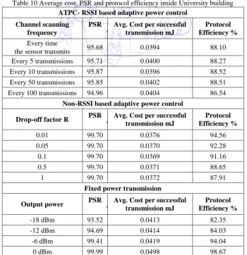
Table 10 shows the average of the performance parameters of the data that were collected. Fig. 12 compares the minimum or the optimal cost of each of the transmission strategies when University building data sets 1, 2 and 3 are used, along with their corresponding PSR and protocol efficiency values. It shows that the non-RSSI based adaptive protocol has proven to be more energy efficient than the fixed power transmission and ATPC. Fig. 12 suggests that the adaptive protocol can save approximately 7% energy as compared to ATPC and can consume 12% less energy than fixed power transmission. The PSR and the protocol efficiency of the non-RSSI based protocol are higher than that of the other two transmission strategies.

Table 10 Average cost, PSR and protocol efficiency inside University building ATPC- RSSI based adaptive power control

Channel scanning frequency

PSR %

Every time

the sensor transmits 95.68 0.0394 88.10

Every 5 transmissions 95.71 0.0400 88.27

Drop-off factor R PSR %

0.01 99.70 0.0376 94.56

0.05 99.70 0.0370 92.28

0.1 99.70 0.0369 91.16

0.5 99.70 0.0371 88.65

1 99.70 0.0372 87.91

Output power PSR

%

-18 dBm 93.52 0.0413 82.35

-12 dBm 94.69 0.0414 84.03

-6 dBm 99.41 0.0419 94.04

(19)

Fig. 12 University building - Comparison of the minimum cost and the corresponding PSR and protocol efficiencies due to different transmission strategy shows that the adaptive protocol can save 7% and 12% energy as compared to ATPC and fixed

power transmission and outperforming the others in terms of PSR and efficiency

7.2 University dining hall with average Eb/N0 reduced by 20 dB

Table 11 has tabulated all the performance parameter values of the data that were collected from University dining hall during busy hours.

Table 11 Average cost, PSR and protocol efficiency inside University dining hall during busy hour ATPC- RSSI based adaptive power control

frequency PSR%

Drop-off factor R PSR% Avg. Cost per successful transmission mJ

0.01 99.53 0.0448 92.20

0.05 99.37 0.0431 89.03

0.1 99.16 0.0431 87.22

0.5 98.98 0.0420 84.25

1 98.97 0.0422 83.04

Output power PSR% Avg. Cost per successful

transmission mJ

-18 dBm 83.84 0.0568 60.59

-12 dBm 86.98 0.0556 63.56

-6 dBm 98.46 0.0462 85.42

(20)

Fig. 13 University dining hall- Comparison of the minimum cost and their corresponding PSR and protocol efficiencies due to different transmission strategy shows that the adaptive protocol consumes 10% less energy than ATPC protocol and fixed power transmission, with comparable PSR and efficiency.

Results of the simulation are shown in Fig. 13. It suggests that the adaptive protocol has emerged out to be the best performer in terms of saving energy. It consumes approximately 10% less energy per successful transmission than ATPC and fixed power transmission.

7.3 Town shopping center with average Eb/N0 reduced by 20 dB

Table 12 has tabulated all the performance parameter values of the data that were collected from University dining hall during busy hours.

Table 12 Average cost, PSR and protocol efficiency inside shopping centre during busy hour ATPC- RSSI based adaptive power control

0.01 99.83 0.0438 92.20

0.05 99.83 0.0419 89.03

0.1 99.8 0.0417 87.22

0.5 99.85 0.0409 84.25

1 99.83 0.0410 83.04

Output power PSR % Avg. Cost per successful

transmission mJ

-18 dBm 83.84 0.0568 60.59

-12 dBm 86.98 0.0556 63.56

-6 dBm 98.46 0.0462 85.42

(21)

Fig. 14 shows that the adaptive protocol has outperformed the ATPC protocol in terms of PSR, protocol efficiency and cost. Referring to Fig. 10, there was enough scope of output power modulation. The occupancy of the link quality around 20 dB (in terms of Eb/N0) is high (more than 20%). The adaptive protocol makes full use of its adaptive power capability to save energy

while maintain a high PSR and protocol efficiency. It is able to save more than 17% energy than ATPC and fixed power transmission.

8. Comparison of PSRs, costs and efficiencies when mean E

b

/N

0

is further reduced by 20 dB

If the mean Eb/N0 is further reduced by 20 dB, then the behavior of the channel is such that it oscillates between a good

channel state (Eb/N0 > 20 dB) and a bad channel state (Eb/N0 ~ 0 dB). The sample normalized frequency distributions of the

Eb/N0 are shown in Fig.15.

Fig. 15 University building- The normalized frequency distribution of the Eb/N0 values

suggests that channel is in bad condition for ~20% of time.

(22)

Fig. 16 University dining hall - The frequency distribution of the Eb/N0 values in during busy

hour shows that the channel quality has oscillated between good and bad. In good state most of the packets will be successfully transmitted, while in bad state almost no packet transmission will be successful

Fig. 17 Town shopping center- The frequency distribution of the Eb/N0 values during busy

hour shows that the channel quality has oscillated between good and bad. In good state most of the packets will be successfully transmitted, while in bad state almost

In such link conditions, the PSR will depend on the occupancy rate of the channel state at or below Eb/N0 of -20 dB. This

is because when the Eb/N0 is -20 dB, power ramping up to 18 dB is not sufficient to make successful packet transmission

possible. All the transmission strategies have approximately similar PSR and protocol efficiency. The fixed power transmission provides the optimal solution in terms of energy required per successful transmission in most of the scenarios that are discussed.

9. Conclusions

The results in this paper demonstrate the advantages and limitations of using power control under different channel conditions to achieve energy efficiency. When the link quality is good (mean Eb/N0 > 55 dB for the lowest power level) with

occasional drop by 20-30 dB due to fading, all the transmission strategies have comparable performances. This is because there was no scope of output power maneuvering to achieve energy efficiency. When the mean Eb/N0 is dropped by 20 dB, the

adaptive power control approach has proved to be energy-saving as compared to fixed power and ATPC when. Under this new channel condition, the mean Eb/N0 is now approximately 30-35 dB and occasional signal drop to 0 dB has resulted in

manipulation of power level. When the mean Eb/N0 is further dropped by 20 dB, it represented a pure two state channel. The

(23)

and most of the packets were successfully transmitted. In the bad state, the average Eb/N0 is -20 dB and all the packets were

dropped. In this type of channel condition, the energy saving solution is provided by the fixed power transmission strategy because any ramping up of output power in bad state will not be sufficient to send a packet successfully. While in good state, it is not required to ramp up power for successful transmission. The non-RSSI approach can be a cost effective solution as compared to a RSSI based channel estimation method (ATPC) when the sensor and the hub are within the communicable distance.

References

[1] M. Weiser, "Ubiquitous computing", http://www.ubiq.com/weiser/UbiHome.html," March 17, 1996. [2] Philips Research - Technologies, "What is ambient intelligence,"

http://www.research.philips.com/technologies/projects/ami/, 2015.

[3] J. P. Sheu, K. Y. Hsieh and Y. K. Cheng, "Distributed transmission power control algorithm for wireless sensor networks," Journal Of Information Science And Engineering, vol. 25, no. 5, pp. 1447-1463, 2009.

[4] S. Lin, J. Zhang, G. Zhou, T. H. Lin Gu and J. A. Stankovic, "ATPC: adaptive transmission power control for wireless sensor networks," in Proc. IEEE SenSys, Oct. 2006, pp. 223-236.

[5] N. Baccour, A. Koubaa, L. Mottola, M. A. Zuniga, H. Youssef, C. A. Boana and M. Alves, "Radio link quality estimation in wireless sensor networks: A Survey," ACM Transactions on Sensor Networks, vol. 8, no. 4, pp. 1-35, 2012.

[6] Chipcon products from Texas Instruments, "2.4 GHz IEEE 802.15.4 / ZigBee-ready RF Transceiver,” http://www.ti.com/lit/ds/symlink/cc2420.pdf, Oct. 2014.

[7] Y. Fu, M. Sha, G. Hackmann and C. Lu, "Practical control of transmission power for wireless sensor networks," Proc. 20th IEEE International Conference on Network Protocols (ICNP ‘12), IEEE press, Oct. 2012, pp. 1-10.

[8] G. Hackmann, O. Chipara and C. Lu, "Robust topology control for indoor wireless sensor networks," Proc. ACM conference on Embedded network sensor systems, 2008, pp. 57-70.

[9] S. Soltani, M. U. Ilyas and H. Radha, "An energy efficient link layer protocol for power-constrained wireless networks," Proc. International Conference on Computer Communications and Networks (ICCCN ‘11), July. 2011, pp. 1-6.

[10] L. Zheng, W. Wang, A. Mathewson, B. O’Flynn and M. Hayes, "An adaptive transmission power control method for wireless sensor networks," in Proc. ISSC, June. 2010, pp. 261-265.

[11] J. Jeong, D. Culler and J. H. Oh, "Empirical analysis of transmission power control algorithms for wireless sensor networks," International Conference on Networked Sensing Systems, 2007, pp. 27-34.

[12] D. Lal, A. Manjeshwar, F. Herrmann, E. Uysal-Biyikoglu and A. Keshavarzian, "Measurement and characterization of link quality metrics in energy constrained wireless sensor networks," Proc. IEEE Global Telecommunications Conference (GLOBECOM ‘03), IEEE press, Dec. 2003, vol. 1, pp. 446-452.

[13] A. Sheth and R. Han, "An implementation of transmit power control in 802.11b Wireless Networks," University of Colorado at Boulder, 2002.

[14] "nRF24L01+ Single Chip 2.4GHz Transceiver Product Specification v1.0," http://www.nordicsemi.com/eng/Products/2.4GHz-RF/nRF24L01P.

[15] D. G. Zhang, Y. N. Zhu, C. P. Zhao, and W. B. Dai, "A new constructing approach for a weighted topology of wireless sensor networks based on local-world theory for the Internet of Things (IOT) ," Computers and Mathematics with Applications, Elsevier, 2012, pp. 1044-1055.

[16] D. G. Zhang and Y. P. Liang, "A kind of novel method of service-aware computing for uncertain mobile applications," Mathematical and Computer Modelling, Elsevier, Jun. 2012, pp. 344-356.

[17] D. G. Zhang, G. Li, K. Zheng, X. C. Min, and Z. H. Pan, "An energy-balanced routing method based on forward-aware factor for wireless sensor networks," IEEE Transactions On Industrial Informatics, vol. 10, no. 1, Feb. 2014, pp. 766-773. [18] D. G. Zhang and X. D. Zhang, "Design and implementation of embedded uninterruptible power supply system (EUPSS) for

web-based mobile application," Enterprise Information Systems, vol. 6, no. 4, pp. 473-489, DOI: 10.1080/17517575.2011.626872.

[19] D. G. Zhang, K. Zheng, T. Zhang, and X. Wang, "A novel multicast routing method with minimum transmission for WSN of cloud computing service," Soft Comput, Springer-Verlag Berlin Heidelberg, pp. 1817–1827, 2014.

(24)

[21] D. G. Zhang, X. Wang, and X. D. Song, “A novel approach to mapped correlation of ID for RFID anti-collision”, IEEE Transactions on Services Computing,” vol. 7, no. 4, pp. 741-748, 2014.

[22] D. G. Zhang, X. D. Song, and X. Wang, “New agent-based proactive migration method and system for big data environment (BDE),” Engineering Computations, vol. 32, no. 8, pp. 2443- 2466, 2015.

[23] D. Basu, G. Sen Gupta, G. Moretti, and X. Gui, "Protocol for improved energy efficiency in wireless sensor networks to support mobile robots," Proc. International Conference on Automation, Robotics and Applications (ICARA), Feb. 2015, pp. 230-237.

[24] D. Basu, G. Sen Gupta, G. Moretti, and X. Gui, “Performance comparison of a novel adaptive protocol with the fixed power transmission in wireless sensor networks,” Journal of Sensor and Actuator Networks, Multidisciplinary Digital Publishing Institute (MDPI AG), pp. 274-292, Sep. 2015.

[25] A. S. Tanenbaum and Computer Networks, Chapter 4, 4th ed., Prentice Hall PTR, 2002. [26] IEEE Standard for Information technology, IEEE Computer Society, 2002.

[27] "Universal Mobile Telecommunications System (UMTS); Selection procedures for the choice of radio transmission technologies of the UMTS (UMTS 30.03 version 3.1.0)," UMTS, 2011.

[28] K. Srinivasan and P. Levis, "RSSI is under appreciated," in Workshop on Embedded Networked Sensors (EmNets), 2006. [29] D. Schmidt, M. Berning, and N. Wehn, "Error correction in single-hop wireless sensor networks - A case study,"

Conference & Exhibition of Design, Automation & Test in Europe, 2009, pp. 1530-1591.

[30] "NetSurveyor — 802.11 Network Discovery / WiFi Scanner," http://nutsaboutnets.com/netsurveyor-wifi-scanner/. [31] "Beacon Frame," http://en.wikipedia.org/wiki/Beacon_frame.

[32] J. Geier, "802.11 Beacons Revealed," http://www.wi-fiplanet.com/tutorials/print.php/1492071, Oct. 2002.