A Study on Different Music Genre Classification Methods

(1)

Impact Factor: 5.515

A Study on Different Music

Genre Classification Methods

Alif Noushad

1

, Albin Paul

2

, Anjana Mukesh

3

, Ebin B Plackal

4

, Mohan T D

5

, Anjali S

6

U.G. Student, Department of Computer Engineering, Model Engineering College, Thrikkakara, Cochin, India1,2,,3,4,5 Assistant Professor, Department of Computer Engineering, Model Engineering College, Thrikkakara, Cochin, India 6

ABSTRACT: Classification of music has acquired much importance and interest in the last decades. Identifying and categorising music by analysing the spectrogram through various methodologies should be a point of research when high accuracy matters in classification. This stage of music analysis plays a major role in recommendation of music in music players. Better understanding of the music gives better results. This paper presents a survey on various music genre classification methods proposed.

Keywords: Genre Classification, Algorithms, Music recommendation

1. Introduction

The rapid development of Internet together with the growth of the bandwidth availability have resulted in the widespread of large amounts of digital multimedia contents in Internet. One of the most important types of multimedia content distributed over the Internet is a high volume of digital music in MP3 format. This has motivated researchers to develop music information retrieval (MIR) techniques that would be helpful for Internet music search engines, musicologist and listeners to find music from numerous options. Among these techniques, automatic classification of music pieces into categories such as mood, artist or genre is widely studied topic in MIR as it is an efficient method to structure and organize the large numbers of music files available on the Internet. A music genre describes a style of music that has similar characteristics shared by its members and can be distinguished from other types of music. These characteristics are usually related to the instrumentation, rhythm, harmony, and melody of the music. Generally, the genre classification process of music has two main steps: feature extraction and classification. The first step obtains audio signal information, while the second one classifies the music into various genres according to extracted features. Chord recognition methods are used for feature extraction from an audio signal. The chord recognition task constructs a chord label from a specific music -related feature. On the other hand, different data-mining algorithms, including supervised, unsupervised and semi-supervised classification, are proposed to classifying music genres. In this paper we present our study on the different techniques that are used for identification of genre of music and classifying them. There are various pure mathematical methods like FFT that are analysed in this paper. There are other methods like Linear predictive coding, MFCC, Perceptual Linear Prediction, RASTA are also elaborated here. Some usual techniques like Support Vector Machine, Decision tree, Nearest Neighbour and RNN are also discussed in this paper.

2. Related Work

A. Linear Predictive Coding

LPC is one of the most powerful speech analysis techniques and is a useful method for encoding quality speech at a low bit rate. The basic idea behind linear predictive analysis is that a specific speech sample at the current time can be approximated as a linear combination of past speech samples.

Methodology

(2)

speech signal and the estimated speech signal over a finite duration. This could be used to give a unique set of predictor coefficients. These predictor coefficients are estimated every frame, which is normally 20 ms long. The predictor coefficients are represented by ak. Another important parameter is the gain (G). The transfer function of the time varying digital filter is given by

H(z) = G/(1-Σakz-k)

Where k=1 to p, which will be 10 for the LPC-10 algorithm and 18 for the improved algorithm that is utilized. Levinson-Durbin recursion will be utilized to compute the required parameters for the autocorrelation method.

The LPC analysis of each frame also involves the decision-making process of voiced or unvoiced. A pitch-detection algorithm is employed to determine to correct pitch period / frequency. It is important to re-emphasise that the pitch, gain and coefficient parameters will be varying with time from one frame to another. In reality the actual predictor coefficients are never used in recognition, since they typical show high variance. The predictor coefficient is transformed to a more robust set of parameters known as cepstral coefficients.

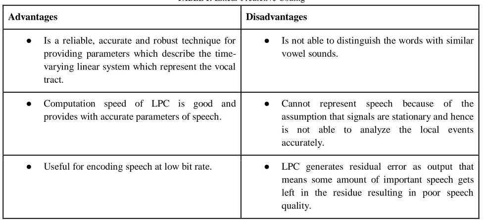
TABLE 1: Linear Predictive Coding

Advantages Disadvantages

● Is a reliable, accurate and robust technique for providing parameters which describe the time-varying linear system which represent the vocal tract.

● Is not able to distinguish the words with similar vowel sounds.

● Computation speed of LPC is good and provides with accurate parameters of speech.

● Cannot represent speech because of the assumption that signals are stationary and hence is not able to analyze the local events accurately.

● Useful for encoding speech at low bit rate. ● LPC generates residual error as output that means some amount of important speech gets left in the residue resulting in poor speech quality.

B. Mel Frequency Cepstral Coefficient (MFCC)

The use of Mel Frequency Cepstral Coefficients can be considered as one of the standard method for feature extraction.[1] The use of about 20 MFCC coefficients is common in automatic speech recognition, although 10-12 coefficients are often considered to be sufficient for coding speech. The most notable downside of using MFCC is its sensitivity to noise due to its dependence on the spectral form. Methods that utilize information in the periodicity of speech signals could be used to overcome this problem, although speech also contains aperiodic content.

Methodology

(3)

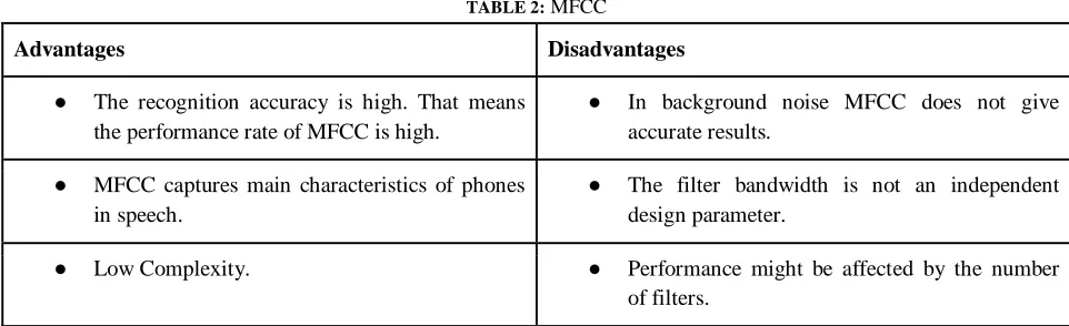
TABLE 2: MFCC

● The recognition accuracy is high. That means the performance rate of MFCC is high.

● In background noise MFCC does not give accurate results.

● MFCC captures main characteristics of phones in speech.

● The filter bandwidth is not an independent design parameter.

● Low Complexity. ● Performance might be affected by the number of filters.

C. LFCC Speech Features

The LFCC is computed as the MFCC-FB40 with the only difference that the Mel frequency warping step is skipped[2]. Thus, the desired frequency range is implemented by a filter-bank of 40 equal-width and equal height linearly spaced filters. The bandwidth of each filter is 164 Hz, and the whole filterbank covers the frequency range [133, 6857] Hz. Obviously, the equal bandwidth of all filters renders unnecessary the effort for normalization of the area under each filter.

Computation of the LFCC

1. The N - point DFT is applied on the discrete time domain input signal x(n). 2. The filter bank is applied on the magnitude spectrum [absolute value of x (k)]. 3. The logarithmically compressed filterbank outputs are computed.

4. Finally, the DCT is applied on the filterbank outputs to obtain the LFCC FB-40 parameters. 5. Analogically to the MFCC FB-40 we compute only the first J = 13 parameters.

TABLE 3: LFCC

● LFCC outperform MFCC for error and recognition rates such as in women‟s voices.

● MFCC is slightly better with interference from white noise compared to LFCC.

● LFCC is slightly better with interference from mumbling noise compared to MFCC.

● LFCC inherits the disadvantages from the LPC technique.

D. Pure FFT

Despite the popularity of MFCCs and LPC, direct use of vectors containing coefficients of FFT power-spectrum are also possible for feature extraction. As compared to methods exploiting knowledge about the human auditory system, the pure FFT spectrum carries comparatively more information about the speech signal. However, much of the extra information is located at the relatively higher frequency bands when using high sampling rates (e.g., 44.1 kHz etc.), which are not usually considered to be salient in speech recognition. The logarithm of the FFT spectrum is also often used to model loudness perception.

TABLE 4: Pure FFT

● The FFT is significantly faster that a DFT in practical power applications.

(4)

● The speed which it gets by decreasing the number of calculations needed to analyze a waveform is higher.

● The restricted range of waveform data that can be transformed and the need to apply a window weighting function (to be defined) to the waveform to compensate for spectral leakage (also to be defined).

E. Power Spectral Analysis(FFT)

One of the more common techniques of studying a speech signal is via the power spectrum. The power spectrum of a speech signal describes the frequency content of the signal over time. The first step towards computing the power spectrum of the speech signal is to perform a Discrete Fourier Transform (DFT). A DFT computes the frequency information of the equivalent time domain signal. Since a speech signal contains only real point values, we can use a real-point Fast Fourier Transform (FFT) for increased efficiency. The resulting output contains both the magnitude and phase information of the original time domain signal.

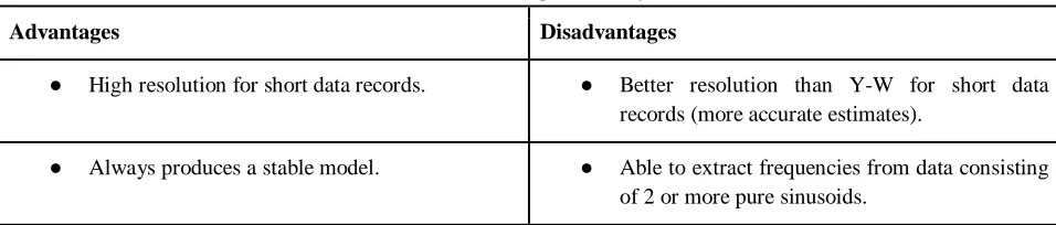
TABLE 5: Power Spectral Analysis

● High resolution for short data records. ● Better resolution than Y-W for short data records (more accurate estimates).

● Always produces a stable model. ● Able to extract frequencies from data consisting of 2 or more pure sinusoids.

F. Perceptual Linear Prediction (PLP)

The Perceptual Linear Prediction PLP model developed by Hermansky 1990. The goal of the original PLP model is to describe the psychophysics of human hearing more accurately in the feature extraction process. PLP is similar to LPC analysis, is based on the short-term spectrum of speech. In contrast to pure linear predictive analysis of speech, perceptual linear prediction (PLP) modifies the short-term spectrum of the speech by several psychophysically based transformations.

PLP Speech Features

The PLP parameters rely on Bark-spaced filterbank of 18 filters for covering the frequency range Hz. Specifically, the PLP coefficients are computed as follows:

● The discrete time domain input signal x(n) is subject to the N - point DFT.

● The critical-band power spectrum is computed through discrete convolution of the power spectrum with the piecewise approximation of the critical-band curve, where B is the Bark warped frequency obtained through the Hertz to Bark conversion.

● Equal loudness pre-emphasis is applied on the down-sampled. ● Intensity-loudness compression is performed.

● The result obtained so far an inverse DFT is performed to obtain the equivalent autocorrelation function. ● Finally, the PLP coefficients are computed after autoregressive modeling and conversion of the autoregressive

coefficients to cepstral coefficients.

TABLE 6: PLP

● PLP coefficients are often used because they approximate well the high-energy regions of the speech spectrum while simultaneously smoothing out the fine harmonic structure, which is often characteristic of the individual but not of the underlying linguistic unit.

● In standard PLP analysis power root constant is 0.33. Its increase towards square root (0.5)

(5)

● PLP incorporates critical-band spectral resolution into its spectrum estimate by remapping the frequency axis to the Bark scale and integrating the energy in the critical bands to produce a critical-band spectrum approximation.

● The spectral sensitivity of PLP-reflection coefficients perform poorly when linearly quantized, especially as the magnitude of reflection coefficients approach unity.

G. Relative Spectral Filtering(RASTA)

To compensate for linear channel distortions the analysis library provides the ability to perform RASTA filtering. The RASTA filter can be used either in the log spectral or cepstral domains. In effect the RASTA filter band passes each feature coefficient. Linear channel distortions appear as an additive constant in both the log spectral and the cepstral domains. The high-pass portion of the equivalent band pass filter alleviates the effect of convolutional noise introduced in the channel. The low-pass filtering helps in smoothing frame to frame spectral changes.

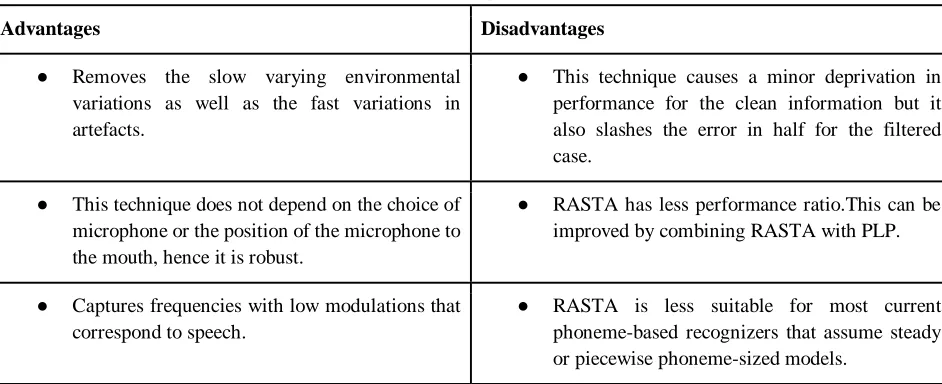
TABLE 7: Relative Spectral Filtering

● Removes the slow varying environmental variations as well as the fast variations in artefacts.

● This technique causes a minor deprivation in performance for the clean information but it also slashes the error in half for the filtered case.

● This technique does not depend on the choice of microphone or the position of the microphone to the mouth, hence it is robust.

● RASTA has less performance ratio.This can be improved by combining RASTA with PLP.

● Captures frequencies with low modulations that correspond to speech.

● RASTA is less suitable for most current phoneme-based recognizers that assume steady or piecewise phoneme-sized models.

H. Logistic Regression

In problems where we need to predict the probability of an outcome that only has two values, we use logistic regression[8]. The prediction is based on the usage of numerical or categorical predictors. A logistic curve is produced whose values are between 0 and 1. The natural log of odds of the target variable is used to plot the logistic curve. The predictors in each group need not be normally distributed or have equal variance. This problem is a multi-classification problem. So we use the one vs all model for logistic regression during implementation. The logistic regression equation is written in terms of an odds ratio by using a simple transformation as:

p/(1-p)=exp(b0+b1x)

In the equation b0 is the regression constant and b1 is the slope of the logistic curve. b1 defines the steepness of the curve. By taking the natural log on both sides, a linear equation of the predictors is derived which can be written in terms of log-odds (logit):

ln(p/(1-p))=b0+b1x

TABLE 8: Logistic Regression

● If the signal to noise ratio is low (it is a „hard‟ problem) logistic regression is likely to perform best. In technical terms, if the AUC of the best model is below 0.8, logistic very clearly outperformed tree induction.

(6)

● You have have low signal to noise for a number of reasons - the problem is just inherently unpredictable (think stock market) dataset or it is too small to „find the signal‟. The latter is an interesting case - we observe that the performance order of the two algorithms can cross - meaning, logistic performs better on a small version of the dataset but eventually is beaten by the tree when the dataset gets large enough.

● Logistic regression requires that each data point be independent of all other data points. If observations are related to one another, then the model will tend to overweight the significance of those observations.

● Trees generally have a harder time coming up with calibrated probabilities. This can be helped somewhat with bagging and Laplace correction.

● Logistic regression attempts to predict outcomes based on a set of independent variables, but logit models are vulnerable to overconfidence. That is, the models can appear to have more predictive power than they actually do as a result of sampling bias.

I. Support Vector Machine

Support Vector Machine (SVM) classifies by finding the hyperplane which maximizes the margin between the two classes.[5] The hyperplane is defined using vectors called support vectors. Optimal hyperplane is started at the beginning of a SVM, it may have a penalty term for misclassifications. The data is mapped to a high dimensional space at the end.

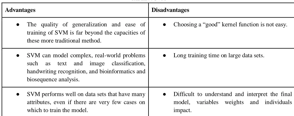
TABLE 9: SVM

● The quality of generalization and ease of training of SVM is far beyond the capacities of these more traditional method.

● Choosing a “good” kernel function is not easy.

● SVM can model complex, real-world problems such as text and image classification, handwriting recognition, and bioinformatics and biosequence analysis.

● Long training time on large data sets.

● SVM performs well on data sets that have many attributes, even if there are very few cases on which to train the model.

● Difficult to understand and interpret the final model, variables weights and individuals impact.

J. Decision Tree

Regression or classification models are constructed as tree structure using decision tree. Dataset is divided into smaller subsets and simultaneously a decision tree is incrementally developed. A decision node has two or more branches. The leaf node in the tree represents a decision or classification. The topmost decision node is called as the root node and corresponds to the predictor. Building decision trees is done by the algorithm called ID3. It makes use of a top-down, greedy search through the space of possible branches with no backtracking. Entropy and information gain is used by ID3 to build a decision tree.A decision tree is constructed top-down from a root node and entails partitioning of data into subsets containing instances with similar values.Samples homogeneity is calculated by ID3 algorithm using entropy. If the sample is totally homogeneous then entropy will be 0 and entropy will be 1 if it‟s equally divided. Entropy for a single variable using frequency table can be calculated by the following equations

E(S)=Σc j=1|xi -yi| Entropy for two variables using frequency table

(7)

TABLE 10: Decision Tree

● Implicitly perform variable screening or feature selection.

● While decision trees are generally robust to outliers, due to their tendency to overfit, they are prone to sampling errors.

● Require relatively little effort from users for data preparation.

● Tree splitting is locally greedy.

● Nonlinear relationships between parameters do not affect tree performance.

● Optimal decision tree is NP-complete problem.

K. K - Nearest Neighbour

K - Nearest Neighbors (K - NN) is one of the basic yet essential classification algorithm in machine learning useful in pattern recognition, data mining and intrusion detection.[8] This algorithm is non-parametric method which doesn‟t make any underlying assumptions about the distribution of data. K - NN is a type of instance based learning (memory-based learning),is a set of algorithms which compares new problem instances with instances seen in training. It is the simplest machine learning algorithms in which the function is only approximated locally and all computation is deferred until classification. To determine which of the K instances in the training dataset are most similar to a new input, a distance measure is used. For real-valued input variables, the most popular distance measure is Euclidean distance.

Euclidean distance is calculated as the square root of the sum of the squared differences between a new point (x) and an existing point (xi) across all input attributes j.

EuclideanDistance(x, xi) = sqrt( sum( (xj – xij)^2 ) )

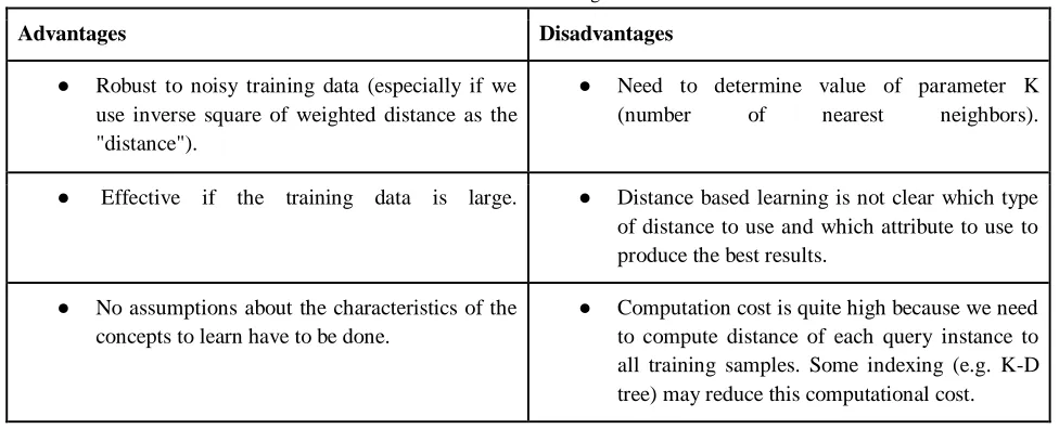
TABLE 11:Nearest Neighbour

● Robust to noisy training data (especially if we use inverse square of weighted distance as the "distance").

● Need to determine value of parameter K (number of nearest neighbors).

● Effective if the training data is large. ● Distance based learning is not clear which type of distance to use and which attribute to use to produce the best results.

● No assumptions about the characteristics of the concepts to learn have to be done.

● Computation cost is quite high because we need to compute distance of each query instance to all training samples. Some indexing (e.g. K-D tree) may reduce this computational cost.

L. Recurrent Neural Network

(8)

The most commonly used type of RNNs are LSTM Networks (Long short-term memory). It is used to revolutionize speech recognition, improve vocabulary and text-to-speech synthesis, which was used In google android.

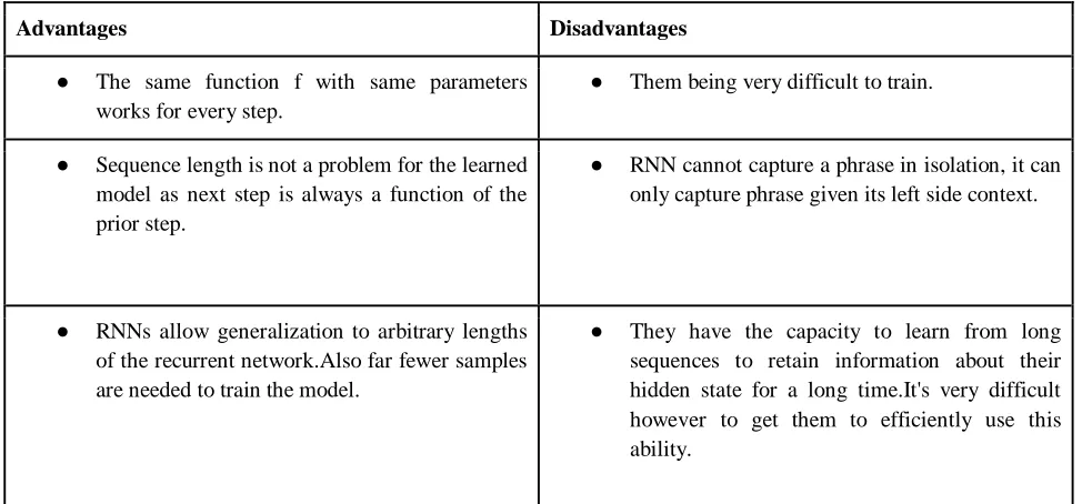
TABLE 12: Recurrent Neural Network

● The same function f with same parameters works for every step.

● Them being very difficult to train.

● Sequence length is not a problem for the learned model as next step is always a function of the prior step.

● RNN cannot capture a phrase in isolation, it can only capture phrase given its left side context.

● RNNs allow generalization to arbitrary lengths of the recurrent network.Also far fewer samples are needed to train the model.

● They have the capacity to learn from long sequences to retain information about their hidden state for a long time.It's very difficult however to get them to efficiently use this ability.

3. Conclusion

In this paper, we presented an extensive survey on various Music Genre Classification techniques. From the above study we can infer that using MFCC data values gives better results overall than using FFT values. PLP and MFCC are derived on the concept of logarithmically spaced filterbank, clubbed with the concept of human auditory system hence has better performance. The Simpler algorithms such as Logistic Regression and K Nearest Neighbors did fairly well compared to superior algorithms such as Recurrent Neural Networks and Support Vector Machines. Pattern matching is efficiently done using Recurrent Neural Networks. All others techniques discussed above fails to produce pattern matching as efficient as Recurrent Neural Networks. Performance of technique like RASTA is increased by combining RASTA with PLP hence ensuring better performance ratio.

References

[1] Convolutional Recurrent Neural Network for Music Classification , Keunwoo Choi, Gyorgy Fazekas, Mark Sandler, Kyunghyun Cho, 2017

[2] Ranking-based Music Recommendation in Online Music Radios, Yao Lu,Zhi Qiao,Peng Zhang,Li Guo,2016 [3] Music Recommendation via Heterogeneous Information Graph Embedding ,Neural Networks (IJCNN), 2017

International Joint Conference on

[4] Music emotion recognition using PSO-based fuzzy hyper-rectangular composite neural networks, Yu-Hao Chin, Yi-Zeng Hsieh, Mu-Chun Su, Shu-Fang Lee, Miao-theyn Chen, Jia-Ching Wang, 2017

[5] A Music Identification System Based on Audio Fingerprint, Consumer Electronics (ICCE), 2015 IEEE International Conference

[6] Personalized Music Recommendation Algorithm Based on Tag Information, Applied Computing and Information Technology, 2016 4th Intl Conf

[7] Learning Content Similarity for Music Recommendation, 2016 7th IEEE International Conference on Software Engineering and Service Science (ICSESS)

[8] A comparative study of classifiers for music genre classification based on feature extractors, IEEE Transactions on Audio, Speech, and Language Processing ( Volume: 20, Issue: 8, Oct. 2012 )