A Direct Estimation of High Dimensional Stationary Vector Autoregressions

A Direct Estimation of High Dimensional Stationary Vector

Autoregressions

Fang Han [email protected]

Department of Biostatistics Johns Hopkins University Baltimore, MD 21205, USA

Huanran Lu [email protected]

Han Liu [email protected]

Department of Operations Research and Financial Engineering Princeton University

Princeton, NJ 08544, USA

Editor:Xiaotong Shen

Abstract

The vector autoregressive (VAR) model is a powerful tool in learning complex time series and has been exploited in many fields. The VAR model poses some unique challenges to researchers: On one hand, the dimensionality, introduced by incorporating multiple numbers of time series and adding the order of the vector autoregression, is usually much higher than the time series length; On the other hand, the temporal dependence structure naturally present in the VAR model gives rise to extra difficulties in data analysis. The regular way in cracking the VAR model is via “least squares” and usually involves adding different penalty terms (e.g., ridge or lasso penalty) in handling high dimensionality. In this manuscript, we propose an alternative way in estimating the VAR model. The main idea is, via exploiting the temporal dependence structure, formulating the estimating problem to a linear program. There is instant advantage of the proposed approach over the lasso-type estimators: The estimation equation can be decomposed to multiple sub-equations and accordingly can be solved efficiently using parallel computing. Besides that, we also bring new theoretical insights into the VAR model analysis. So far the theoretical results developed in high dimensions (e.g., Song and Bickel, 2011 and Kock and Callot, 2015) are based on stringent assumptions that are not transparent. Our results, on the other hand, show that the spectral norms of the transition matrices play an important role in estima-tion accuracy and build estimaestima-tion and predicestima-tion consistency accordingly. Moreover, we provide some experiments on both synthetic and real-world equity data. We show that there are empirical advantages of our method over the lasso-type estimators in parameter estimation and forecasting.

Keywords: transition matrix, multivariate time series, vector autoregressive model, double asymptotic framework, linear program

1. Introduction

analysis (Vald´es-Sosa et al., 2005). For example, in understanding the brain connectivity network, multiple resting-state functional magnetic resonance imaging (rs-fMRI) data are obtained by consecutively scanning the same subject for approximately a hundred times or more. This naturally produces a high dimensional dependent data and a common strategy in handling such data is via building a vector autoregressive model (see Qiu et al., and the references therein).

This manuscript considers estimating the VAR model. Our focus is on the stationary vector autoregression with the order (or called lag)pand Gaussian noises. More specifically, let random vectors X1, . . . , XT be from a stochastic process (Xt)∞t=−∞. Each Xt is a d

-dimensional random vector and satisfies that

Xt= p

X

k=1

AT

kXt−k+Zt, Zt∼Nd(0,Ψ),

where A1, . . . , Ap are called the transition matrices and (Zt)∞t=−∞ are independent multi-variate Gaussian noises. Via assuming det(Id−Pp_k=1ATkzk)6= 0 for allz∈ C with modulus

not greater than one, we then have the process is stationary (check, for example, Section 2.1 in L¨utkepohl, 2005) and Xt ∼ Nd(0,Σ) for some covariance matrix Σ depending on

{Ak, k= 1, . . . , p} and Ψ.

There are in general three main targets in analyzing an VAR model. One is to es-timate the transition matrices A1, . . . , Ap. These transition matrices reveal the temporal

dependence in the data sequence and estimating them builds a fundamental first step in forecasting. Moreover, the zero and nonzero entries in the transition matrices directly in-corporate the Granger non-causalities and causalities with regard to the stochastic sequence (see, for example, Corollary 2.2.1 in L¨utkepohl, 2005). Another one of interest is the error covariance Ψ, which reveals the contemporaneous interactions amongdtime series. Finally, by merely treating the temporal dependence as another measure of the data dependence (in parallel to the mixing conditions, Bradley, 2005), it is also of interest to estimate the covariance matrix Σ.

This manuscript focuses on estimating the transition matrices A1, . . . , Ap, while noting

that the techniques developed here can also be exploited to estimate the covariance matrix Σ and the noise covariance Ψ. We first review the methods developed so far in transition matrix estimation. Let A = (AT

1, . . . , A T

p)T ∈ Rdp×d be the combination of the transition

matrices. Given X1, . . . , XT, the perhaps most classic method in estimating A is least

squares minimization (Hamilton, 1994)

b

ALSE= argmin

M∈_Rdp×d

kYe −MTXek2_F, (1)

where k · k_F is the matrix Frobenius norm, Ye = (X_p+1, . . . , X_T) ∈ Rd×(T−p), and Xe = {(XT

p, . . . , X1T)T, . . . ,(XTT−1, . . . , XTT−p)T} ∈R(dp)×(T−p). However, a fatal problem in (1) is

the estimator: From the ridge-penalty to the lasso-penalty and more non-concave penalty terms. In the following we list the major efforts. Hamilton (1994) discussed the use of the ridge-penalty kMk2

F in estimating the transition matrices. Hsu et al. (2008) proposed to add the L1-penalty in estimating the transition matrices, inducing a sparse output. Several extensions to transition matrix estimation in the VAR model include: Wang et al. (2007) exploited theL1-penalty in simultaneously estimating the regression coefficients and determining the number of lags in a linear regression model with autoregressive errors. In detecting causality, Haufe et al. (2008) transferred the problem to estimating transition matrices in an VAR model and advocated using a group-lasso penalty for inducing joint sparsity among a whole block of coefficients. In studying the graphical Granger causality problem, Shojaie and Michailidis (2010) exploited the VAR model and proposed to estimate the coefficients using a truncated weighted L1-penalty. Song and Bickel (2011) exploited the L1 penalty in a complicated VAR model and aimed to select the variables and lags simultaneously.

The theoretical properties of the L1-regularized estimator have been analyzed in Bento et al. (2010), Nardi and Rinaldo (2011), Song and Bickel (2011), and Kock and Callot (2015) under the assumption that the matrix A is sparse, i.e., the number of nonzero entries in Ais much less than the dimension of parameters pd2. Nardi and Rinaldo (2011) provided both subset and parameter estimation consistency results under a relatively low dimensional settings withd=o(n1/2). Bento et al. (2010) studied the problem of estimating supports sets of the transition matrices in the high dimensional settings and proposed an “irrepresentable condition” similar as what is proposed in the linear regression model (Zou, 2006; Zhao and Yu, 2006; Meinshausen and B¨uhlmann, 2006; Wainwright, 2009). It is for the L1 regularized estimator to attain the support set selection consistency. In parallel, Song and Bickel (2011) and Kock and Callot (2015) studied the parameter estimation and support set selection consistency of the L1-regularized estimator in high dimensions.

In this paper, we propose a new approach to estimate the transition matrixA. Different from the line of lasso-based estimation procedures, which are built on penalizing the least square term, we exploit the linear programming technique and the proposed method is very fast to solve via parallel computing. Moreover, we do not need A to be exactly sparse and allow it to be only “weakly sparse”. The main idea is to estimate A using the relationship between A and the marginal and lag 1 autocovariance matrices (such a relationship is referred to as the Yule-Walker equation). We thus formulate the estimation procedure to a linear program, while adding the k · kmax (element-wise supremum norm) for model identifiability. Here we note that the proposed procedure can be considered as a generalization of the Dantzig selector (Candes and Tao, 2007) to the linear regression model with multivariate response. Indeed, our proposed method can also be exploited in conducting multivariate regression (Breiman and Friedman, 1997).

matrix for example, which are not transparent and do not explicitly reveal the role of temporal dependence in it. In contrast, we provide explicit nonasymptotic analysis, and our analysis highlights the spectral normkAk₂ in estimation accuracy, which is inspired by some recent developments (Loh and Wainwright, 2012). Moreover, for exact sign recovery, our analysis does not need the “irrepresentable condition” which is usually required in the analysis of lasso-type estimators (Bento et al., 2010).

The major theoretical results are briefly stated as follows. We adopt a double asymptotic framework where d is allowed to increase with T. We call a matrix s-sparse if there are at most s nonzero elements on each of its column. Under mild conditions, we provide the explicit rates of convergence of our estimatorAbbased on the assumption thatAiss-sparse (Cai et al., 2011). In particular, for lag 1 time series, we show that

kAb−Ak₁ =O_P (

skAk1 1− kAk2

logd

T

1/2)

, kAb−Ak_max=O_P (

kAk1 1− kAk2

logd

T

1/2)

,

where k · kmax and k · kq represent the matrix elementwise absolute maximum norm (Lmax norm) and induced Lq norm (detailed definitions will be provided in §2). Using theLmax norm consistency result, we further provide the sign recovery consistency of the proposed method. This result is of self interest and sheds light to detecting Granger causality. We also provide the prediction consistency results based on theL1 consistency result and show that element-wise error in prediction can be controlled. Here for simplicity we only provide the results when A is exactly sparse and defer the presentation of the results for weakly sparse matrix to Section 4.

The rest of the paper is organized as follows. In Section 2, we briefly review the vector autoregressive model. In Section 3, we introduce the proposed method for estimating the transition matrices of the vector autoregressive model. In Section 4, we provide the main theoretical results. In Section 5, we apply the new method to both synthetic and real equity data for illustrating its effectiveness. More discussions are provided in the last section. Detailed technical proofs are provided in the appendix1.

2. Background

In this section, we briefly review the vector autoregressive model. Let M = (Mjk) ∈Rd×d

and v = (v1, ..., vd)T ∈ Rd be a matrix and an vector of interest. We denote vI to be the

subvector ofvwhose entries are indexed by a setI ⊂ {1, . . . , d}. We also denoteMI,J to be

the submatrix ofM whose rows are indexed byI and columns are indexed byJ. We denote

MI,∗ to be the submatrix ofM whose rows are indexed byI, M∗,J to be the submatrix of

M whose columns are indexed byJ. For 0< q <∞, we define the L0,Lq, andL∞ vector (pseudo-)norms to be

kvk₀:=

d

X

j=1

I(vj 6= 0), kvkq :=

Xd

j=1

|vj|q

1/q

, and kvk∞:= max 1≤j≤d|vj|,

whereI(·) is the indicator function. LettingM be a matrix, we denote the matrixLq,Lmax, and Frobenius norms to be

kMkq:= max kvkq=1

kM vkq, kMkmax:= max

jk |Mjk|, and kMkF :=

X

j,k

|Mjk|2

1/2

.

We denote 1d= (1, . . . ,1)T∈Rd. Letσ1(M)≥ · · · ≥σd(M) be the singular values ofM.

Let p ≥ 1 be an integer. A lag p vector autoregressive process can be elaborated as follows: Let (Xt)∞t=−∞ be a stationary sequence of random vectors in Rdwith mean 0 and covariance matrix Σ. We say that (Xt)∞t=−∞ follow a lag p vector autoregressive model if and only if they satisfy

Xt= p

X

k=1

AT

kXt−k+Zt (t∈Z). (2)

Here A1, . . . , Ap are called transition matrices. We denote A = (AT1, . . . , ATp)T to be the

combination of the transition matrices. We assume thatZtare independently and identically

generated from a Gaussian distributionNd(0,Ψ). Moreover,Ztand (Xs)s<tare independent

for any t ∈ Z. We pose an additional assumption that det(Id−P_kp₌₁AT_kzk) 6= 0 for all

z∈ C with modulus not greater than one. This guarantees that the sequence is stationary and we have, for anyt∈_Z,Xtfollows a Gaussian distribution Nd(0,Σ),

We denote Σi(·) to be an operator on the process (Xt)∞t=−∞. In particular, we define Σi{(Xt)} = Cov(X0, Xi). It is easy to see that Σ0{(Xt)} = Σ. If the lag of the vector

autoregressive model is 1 (i.e.,Xt=AT1Xt−1+Zt, for any t∈Z), by simple calculation we

have the so called “Yule-Walker Equation”

Σi{(Xt)}= Σ0{(Xt)}(A1)i, (3) which further implies that

A1= [Σ0{(Xt)}]−1·Σ1{(Xt)}.

The results for lag 1 vector autoregressive model can be extended to the lag p vector autoregressive model by appropriately redefining the random vectors. In detail, the autore-gressive model with lagpshown in (2) can be reformulated as an autoregressive model with lag 1

e

Xt=AeTXe_t−1+Ze_t, (4) where

e

Xt=



   

Xt+p−1

Xt+p−2 .. . Xt     

, Ae= 

   

A1 Id 0 . . . 0

..

. . .. · · · ...

Ap−1 0 0 . . . Id

Ap 0 0 . . . 0



   

, Ze_t= 

   

Zt+p−1 0 .. . 0      . (5)

Here Id∈Rd×dis the identity matrix,Xe_t∼N_dp(0,Σ) fore t= 1, . . . , T, and Ze_t∼N_dp(0,Ψ)e withΣ = Cov(e Xe_t) andΨ = Cov(e Ze_t). Therefore, we also have

e

3. Methods and Algorithms

We provide a new formulation to estimate A1, . . . , Ap for the vector autoregressive model.

Let X1, . . . , XT be from a lag p vector autoregressive process (Xt)∞t=−∞ and we denote e

Xt= (XtT+p−1, . . . , XtT)T fort= 1, . . . , T −p+ 1. We denote S and S1 to be the marginal and lag 1 sample covariance matrices of (Xe_t)T

−p+1 t=1

S := 1

T −p+ 1 T−p+1

X

t=1 e

XtXe_tT, S₁ := 1

T −p

T−p

X

t=1 e

XtXe_tT₊₁. (7)

Using the connection between Ae and Σ₀{(Xe_t)},Σ₁{(Xe_t)} shown in (6), we know that a good estimator ˇΩ of Aeshall satisfy that

kΣ0{(Xe_t)}Ωˇ −Σ₁{(Xe_t)}k (8) is small enough with regard to a certain matrix norm k · k. Moreover, using the fact that

A= (AT

1, . . . , ATp)T=Ae_∗,J, whereJ ={1, . . . , d}, by (8) we have that a good estimate ˇA of

A shall satisfy

kΣ0{(Xet)}Aˇ−[Σ1{(Xet)}]∗,Jk (9)

is small enough.

Motivated by (9), we estimateA1, . . . , Ap via replacing Σ0{(Xe_t) and [Σ₁{(Xe_t)}]∗,J with

their empirical versions. For formulating the estimation equation to a linear program, we use theLmax norm. Accordingly, we end in solving the following convex optimization program

b

Ω = argmin

M∈Rdp×d

X

jk

|Mjk|, subject to kSM−(S1)∗,Jkmax≤λ0, (10)

where λ0 >0 is a tuning parameter. In (10), the constraint part aims to find an estimate that approximates the true parameter well, and combined with the minimization part, aims to induce certain sparsity. Let Ωb_∗,j =βb_j, it is easy to see that (10) can be decomposed to many subproblems and each βb_j can be solved by

b

βj = argmin v∈_Rdp

kvk₁, subject to kSv−(S1)∗,jk∞≤λ0. (11)

Accordingly, compared to the lasso-type procedures, the proposed method can be solved in parallel and therefore is computationally more efficient.

Once Ω is obtained, the estimator of the transition matrixb A_k can then be written as

b

Ak=Ωb_J

k,∗, (12)

where we denoteJk={j:d(k−1) + 1≤j≤dk}.

We now show that the optimization in (11) can be formulated into a linear program. Recall that any real numberatakes the decompositiona=a+−a−, wherea+=a·I(a≥0) and a−=−a·I(a <0). For any vectorv= (v1, . . . , vd)T∈Rd, let v+= (v+1, . . . , vd+)

T _and

v−= (v₁−, . . . , v−_d)T_{. We denote v≥0 if v}

ifv1−v2≥0, andv1< v2 ifv1−v2 <0. Lettingv= (v1, . . . , vd)T, the problem in (11) can

be further relaxed to the following problem

b

βj = argmin v+_,v−

1T

d(v++v−),

subject to kSv+−Sv−−(S1)∗,jk∞≤λ0, v+ ≥0, v−≥0. (13) To minimize 1T

d(v++v

−_{), v}+ _{or v}− _{can not be both nonzero. Therefore, the solution to} (13) is exactly the solution to (11). The optimization in (13) can be written as

b

βj = argmin v+_,v−

1T

d(v++v−),

subject to Sv+−Sv−−(S1)∗,j ≤λ01d,

−Sv++Sv−+ (S1)∗,j ≤λ01d,

v+ ≥0, v−≥0.

This is equivalent to

b

βj = argmin ω

1T

2dω, subject to θ+W ω≥0, ω ≥0, (14)

where

ω =

v+ v−

, θ=

(S1)∗,j+λ01d

−(S1)∗,j+λ01d

, W =

−S S

S −S

.

The optimization (14) is a linear program. We can solve it using the simplex algorithm (Murty, 1983).

4. Theoretical Properties

In this section, under the double asymptotic framework, we provide the nonasymptotic rates of convergence in parameter estimation under the matrixL1 and Lmax norms.

We first present the rates of convergence of the estimator Ω in (10) under the vectorb autoregressive model with lag 1. This result allows us to sharply characterize the impact of the temporal dependence of the time series on the obtained rate of convergence. In particular, we show that the rate of convergence is closely related to the L1 and L2 norms of the transition matrix A1, where kA1k2 is the key part in characterizing the impact of temporal dependence on estimation accuracy. Secondly, we present the sign recovery consistency result of our estimator. Compared to the lasso-type estimators, our result does not require the irrepresentable condition. These results are combined together to show that we have the prediction consistency, i.e., the termkA1XT −Ab₁X_Tkgoes to zero with regard to certain norms k · k. The application to lagp >1 case is left for future studies.

We start with some additional notation. Let Md ∈ R be a quantity which may scale

with the time series length and dimension (T, d). We define the set of square matrices in

Rd×d, denoted byM(q, s, Md), as

M(q, s, Md) :=

n

M ∈Rd×d: max 1≤j≤d

d

X

i=1

|Mij|q ≤s,kMk1 ≤Md

o

Forq= 0, the classM(0, s, Md) contains all thes-sparse matrices with boundedL1 norms. There are two general remarks about the model M(q, s, Md): (i) M(q, s, Md) can be

considered as the matrix version of the vector “weakly sparse set” explored in Raskutti et al. (2011) and Vu and Lei (2012). Such a way to define the weakly sparse set of matrices is also investigated in Cai et al. (2011). (ii) For the exactly sparse matrix set, M(0, s, Md),

the sparsity level s here represents the largest number of nonzero entries in each column of the matrix. In contrast, the sparsity level s0 exploited in Kock and Callot (2015) is the total number of nonzero entries in the matrix. We must have s0 ≥s and regularlys0 s

(meanss/s0 →0).

The next theorem presents theL1andLmaxrates of convergence of our estimator under the vector autoregressive model with lag 1.

Theorem 1 Suppose that(Xt)Tt=1 are from a lag 1 vector autoregressive process (Xt)∞t=−∞ as described in (2). We assume the transition matrixA1 ∈ M(q, s, Md)for some0≤q <1. Let Ab₁ be the optimum to (10) with the tuning parameter

λ0=

32kΣk₂maxj(Σjj)

minj(Σjj)(1− kAk2)

(2Md+ 3)

logd

T

1/2

.

For T ≥6 logd+1 and d≥8, we have, with probability no smaller than 1−14d−1,

kAb₁−A₁k₁ ≤4s (

32kΣ−1k1maxj(Σjj)kΣk2 minj(Σjj)(1− kA1k2)

(2Md+ 3)

logd

T

1/2)1−q

. (15)

Moreover, with probability no smaller than 1−14d−1,

kAb₁−A₁k_max≤

64kΣ−1k1maxj(Σjj)kΣk2 minj(Σjj)(1− kA1k2)

(2Md+ 3)

logd

T

1/2

. (16)

In the above results, Σ is the marginal covariance matrix of Xt.

It can be observed that, similar to the lasso and Dantzig selector (Candes and Tao, 2007; Bickel et al., 2009), the tuning parameter λ0 here depends on the variance term Σ. In practice, same as most preceded developments (see, for example, Song and Bickel, 2011), we can use a data-driven way to select the tuning parameter. In this manuscript we explore using cross-validation to choose λ0 with the best prediction accuracy. In Section 5 we will show that the procedure of selecting the tuning parameter via cross-validation gives reasonable results.

HereA1 is assumed to be at least weakly sparse and belong to the setM(q, s, Md). This

is merely for the purpose of model identifiability. Otherwise, we will have multiple global optima in the optimization problem.

The obtained rates of convergence in Theorem 1 depend on both Σ andA1 withkA1k2 characterizing the temporal dependence. In particular, the estimation error is related to the spectral norm of the transition matrix A1. Intuitively, this is because kA1k2 characterizes the data dependence of X1, . . . , XT, and accordingly intrinsically characterizes how much

exploit in estimating A1. Technically, kA1k2 determines the rate of convergence ofS and

S1 to their population counterparts. We refer to the proofs of Lemmas 1 and 2 for details. In the following, we list two examples to provide more insights about the results in Theorem 1.

Example 1 We consider the case where Σ is a strictly diagonal dominant (SDD) matrix (Horn and Johnson, 1990) with the property

δi :=|Σii| −

X

j6=i

|Σij| ≥0, (i= 1, . . . , d).

This corresponds to the cases where the dentries in any Xt with t∈ {1, . . . , T} are weakly dependent. In this setting, Ahlberg and Nilson (1963) showed that

kΣ−1k1=kΣ−1k∞≤ n

min

i

|Σii| −

X

j6=i

|Σij|

o−1

= max

i (δ −1

i ). (17)

Moreover, by algebra, we have

kΣk2 ≤ kΣk1= max i

|Σii|+

X

j6=i

|Σij|

≤2 max

i (|Σii|). (18)

Equations (17)and (18) suggest that, whenmaxi(Σii)is upper bounded, and both mini(Σii) and δi are lower bounded by a fixed constant, we have both kΣ−1k1 and kΣk2 are upper bounded, and the obtained rates of convergence in (15) and (16) can be simplified as

kAb₁−A₁k₁ =O_P 

s (

Md

1− kA1k2

logd T

1/2)1−q 

,

kAb₁−A₁k_max=O_P (

Md

1− kA1k2

logd T

1/2)

.

Example 2 We can generalize the “entry-wise weakly dependent” structure in Example 1 to a “block-wise weakly dependent” structure. More specifically, we consider the case where Σ = (Σb_jk) with blocks Σb_jk ∈ _Rdj×dk _{(1 ≤ j ≤ K) is a strictly block diagonal dominant}

(SBDD) matrix with the property

δb_i =k(Σb_ii)−1k−1_∞ −X

j6=i

kΣb_ijk∞>0 (i= 1, . . . , K).

In this case, Varah (1975) showed that

kΣ−1k1 =kΣ−1k∞≤ n

min

i

k(Σb_ii)−1k−1_∞ −X

j6=i

kΣb_ijk∞ o−1

= max{(δ_ib)−1}.

Moreover, we have

kΣk2≤ kΣk1≤max i (k(Σ

b

Accordingly, generally (k(Σb_ii)−1k−1

∞ +kΣbiik∞) is in the scale of maxi(di)d, and when δib are lower bounded and the condition number of Σ is upper bounded, we have the obtained rates of convergence can be simplified as

kAb₁−A₁k₁ =O_P 

s (

Md·maxi(di)

1− kA1k2

logd T

1/2)1−q 

,

kAb₁−A₁k_max=O_P (

Md·maxi(di)

1− kA1k2

logd T

1/2)

.

We then continue to the results of feature selection. If we have A1 ∈ M(0, s, Md), from

the element-wise Lmaxnorm convergence, a sign recovery result can be obtained. In detail, let ˘A1 be a truncated version of Ab₁ with level γ

( ˘A1)ij = (Ab₁)_ijI{|(Ab₁)_ij| ≥γ}. (19) The following corollary shows that ˘A1recovers the sign ofA1with overwhelming probability. Corollary 1 Suppose that the conditions in Theorem 1 hold and A1 ∈ M(0, s, Md). If we choose the truncation level

γ = 64kΣ −1_k

1maxj(Σjj)kΣk2 minj(Σjj)(1− kA1k2)

(2Md+ 3)

logd

T

1/2

in (19) and with the assumption that

min {(j,k):(A1)jk6=0}

|(A1)jk| ≥2γ,

we have, with probability no smaller than 1−14d−1, sign(A1) = sign( ˘A1). Here for any matrixM,sign(M)is a matrix with each element representing the sign of the corresponding entry in M.

Here we note that Corollary 1 sheds lights to detecting Granger causality. For any two processes {yt} and {zt}, Granger (1969) defined the causal relationship in principle as

follows: Provided that we know everything in the universe, {yt} is said to cause {zt} in

Granger’s sense if removing the information about {ys}s≤tfrom the whole knowledge base

built by timetwill increase the prediction error aboutzt. It is known that the noncausalities

are determined by the transition matrices in the stable VAR process (L¨utkepohl, 2005). Therefore, detecting the nonzero entries ofA1 consistently means that we can estimate the Granger-causality network consistently.

We then turn to evaluate the prediction performance of the proposed method. Given a new data pointXT+1in the time pointT+1, based on (Xt)Tt=1, the next corollary quantifies the distance betweenXT+1 and Ab₁X_T in terms of L_∞ norm.

Corollary 2 Suppose that the conditions in Theorem 1 hold and let

Ψmax:= max

Then for the new data point XT+1 at time point T + 1 and any constant α > 0, with probability greater than

1−2(dα/2−1pπ/2·αlogd})−1−14d−1,

we have

kXT+1−AbT₁X_Tk_∞≤(Ψ_max·αlogd)1/2+ 4s

(

32kΣ−1k₁maxj(Σjj)kΣk2 minj(Σjj)(1− kA1k2)

(2Md+ 3)

logd

T

1/2)1−q

·(Σmax·αlogd)1/2, (20)

where Ab₁ is calculated based on (X_t)T_t=1.

Here we note that the first term in the right-hand side of Equation (20), (Ψmax·αlogd)1/2, is present due to the diverges of the new data point from its mean caused by an unpredictable noise perturb term ZT+1 ∼ Nd(0,Ψ). This term is unable to be canceled out even if we

have almost infinite data points. The second term in the right-hand side of Equation (20) depends on the estimation accuracy of Ab₁ to A₁ and will converge to zero under certain conditions. In other words, the term

kAT

1XT −AbT₁X_Tk∞→0, converges to zero in probability as n, d→ ∞.

AlthoughA1is in general asymmetric, there exist cases such that a symmetric transition matrix is more of interest. It is known that the off-diagonal entries in the transition matrix represent the influence of one state on the others and such influence might be symmetric or not. Weiner et al. (2012) provided several examples where a symmetric transition matrix is more appropriate for modeling the data.

If we can further suppose that the transition matrix A1 is symmetric, we can use this information and obtain a new estimator ¯A1 as

( ¯A1)jk = ( ¯A1)kj := (Ab₁)_jkI(|(Ab₁)_jk| ≤ |(Ab₁)_kj|) + (Ab₁)_kjI(|(Ab₁)_kj| ≤ |(Ab₁)_jk|). In other word, we always pick the entry with smaller magnitudes. Then using Theorem 1, we havekA¯1−A1k1 andkA¯1−A1k∞can be upper bounded by the same number presented in the right-hand side of (15). In this case, because both A1 and ¯A1 are symmetric, we havekA¯1−A1k2≤ kA¯1−A1k1=kA¯1−A1k∞. We then proceed to quantify the prediction accuracy underL2 norm in the next corollary.

Corollary 3 Suppose that the conditions in Theorem 1 hold andA1 is a symmetric matrix. Then for the new data pointXT+1at time pointT+1, with probability greater than1−18d−1, we have

kXT+1−A¯T1XTk2 ≤ p

2kΨk2logd+ p

tr(Ψ) +

4s

(

32kΣ−1k₁maxj(Σjj)kΣk2 minj(Σjj)(1− kA1k2)

(2Md+3)

logd

T

1/2)1−q

· {p2kΣk2logd+ p

tr(Σ)}. (21)

Based on Corollary 3, we have, similar as what is discussed in Corollary 2, the term kAT

5. Experiments

We conduct numerical experiments on both synthetic and real data to illustrate the effec-tiveness of our proposed method compared to the competing ones, as well as obtain more insights on the performance of the proposed method. In the following we consider the three competing methods:

• (i) The least square estimation using a ridge-penalty (The method in Hamilton, 1994, by adding a ridge-penalty kMk2

F to the least squares loss function in Equation 1).

• (ii) The least square estimation using anL1 penalty (The method in Hsu et al., 2008, by adding anL1 penalty

P

ij|Mij|to Equation 1).

• (iii) Our method (The estimator described in Equation 10).

Here we consider including the procedure discussed in Hamilton (1994) because it is a commonly explored baseline and shows how bad the classic procedure can be when the dimension is high. We only consider the competing procedure proposed in Hsu et al. (2008) because this is the only method that is specifically designed for the same simple VAR as what we study. We do not consider other aforementioned procedures (e.g., Haufe et al., 2008; Shojaie and Michailidis, 2010) because they are designed for more specific models with more assumptions. We use the R package “glmnet” (Friedman et al., 2010) for implementing the lasso method in Hsu et al. (2008), and the simplex algorithm for implementing ours.

5.1 Cross-Validation Procedure

We start with an introduction to how to conduct cross-validation for choosing the lagpand the tuning parameterλin the algorithm outlined in Section 3.

For the time series (Xt)Tt=−∞and a specific time pointt0 of interest, if bothpand λare assumed to be unknown, the proposed cross-validation procedure is as follows.

1. We set all possible choices of (p, λ) to be a grid. We setn1 and n2 to be two numbers (representing the length of training data and the number of replicates).

2. For each Xt among Xt0−1, . . . , Xt0−n2, the estimates Abt₁(p, λ), . . . ,Abt_p(p, λ) are cal-culated based on the training data Xt−1, . . . , Xt−n1 and any choice of (p, λ). We set the prediction error at time t, denoted as Errt(p, λ), to be Errt(p, λ) := kXt−

Pp

k=1Abt_k(p, λ)TX_t−kk2.

3. We take an average over the prediction errors and denote

Err(p, λ) := 1

n2 t0−1 X

t=t0−n2

Errt(p, λ)

.

4. We choose the (p, λ) over the grid such that Err(p, λ) is minimized.

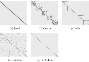
(a) band (b) cluster (c) hub

(d) random (e) scale-free

Figure 1: Five different transition matrix patterns used in the experiments. Here gray points represent the zero entries and black points represent nonzero entries.

5.2 Synthetic Data Analysis

In this subsection, we compare the performance of our method with the ridge and lasso methods using synthetic data under multiple settings. We also study the impact of transi-tion matrices’ spectral norms on estimatransi-tion accuracy, and how the computatransi-tion time and memory usage of all methods scale with the number of lags.

5.2.1 Performance Comparison: Lag p= 1

This section focuses on vector autoregressive model described in (2) with lag one. We compare our method to the competing ones on several synthetic data sets. We consider the settings where the time series length T varies from 50 to 100 and the dimension d varies from 50 to 200.

We create the transition matrix A1 according to five different patterns: band, cluster, hub, random, and scale-free. Typical realizations of these patterns are illustrated in Figure 1 and are generated using the “flare” package in R (Li et al., 2015). In those plots, the gray points represent the zero entries and the black points represent the nonzero entries. We then rescaleA1 such that we have kA1k2 = 0.5. OnceA1 is obtained, we generate Σ using two models. First is the simple setting with Σ to be diagonal

ridge method lasso method our method

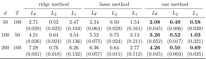
d T LF L2 L1 LF L2 L1 LF L2 L1

50 100 2.71 0.52 2.47 2.34 0.50 1.54 2.08 0.49 0.58 (0.028) (0.023) (0.103) (0.064) (0.029) (0.161) (0.045) (0.006) (0.039) 100 50 4.21 0.64 3.54 5.52 0.75 3.13 3.26 0.52 1.03

(0.026) (0.024) (0.136) (0.075) (0.024) (0.211) (0.052) (0.017) (0.321) 200 100 7.28 0.76 6.26 6.36 0.64 2.77 4.26 0.50 0.69

(0.031) (0.018) (0.132) (0.057) (0.015) (0.112) (0.045) (0.003) (0.035)

Table 1: Comparison of estimation performance of three methods with diagonal covariance matrix over 1,000 replications. The standard deviations are presented in the paren-theses. Here LF, L2, and L1 represent the Frobenius, L2, and L1 matrix norms respectively. The pattern of the transition matrix is “band”.

The second is the complex setting where Σ is of Toeplitz form

Σi,i= 1, Σi,j =ρ|i−j| for someρ∈(0,1) and i, j= 1, . . . , d.

We then calculate the covariance matrix Ψ of the Gaussian noise vector Zt as Ψ = Σ−

AT

1ΣA1. WithA1,Σ, and Ψ, we simulate a time series (X1, . . . , XT)T∈RT×d according to

the model described in (2).

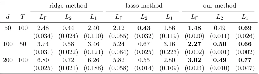
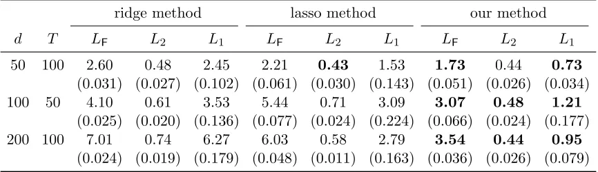
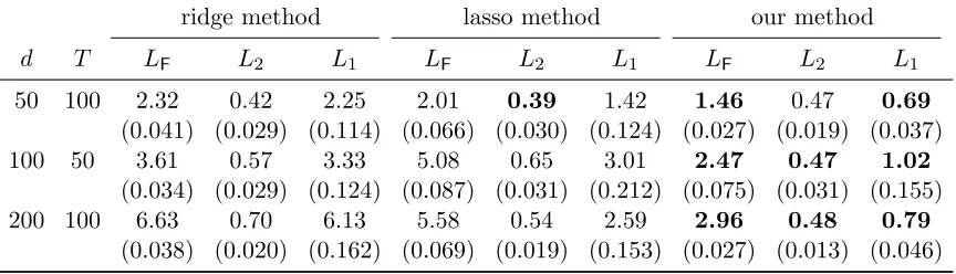
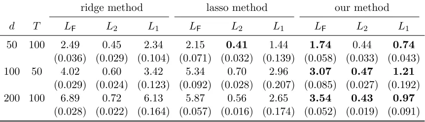
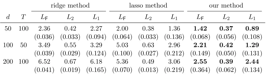
We construct 1,000 replicates and compare the three methods described above. The averaged estimation errors under different matrix norms are illustrated in Tables 1 to 10. The standard deviations of the estimation errors are provided in the parentheses. The tuning parameters for the three methods are selected using the cross-validation procedure outlined in Section 5.1 with n1 =T /2,n2 =T /2, and the lag p predetermined to be 1.

Tables 1 to 10 show that our method nearly uniformly outperforms the methods in Hsu et al. (2008) and Hamilton (1994) under different norms (Frobenius, L2, and L1 norms). In particular, the improvement over the method in Hsu et al. (2008) tends to be more significant when the dimension d is larger. Our method also has averagely slightly less standard deviations compared to the method in Hsu et al. (2008), but overall the difference is not significant. The method in Hamilton (1994) has worse performance than the other two methods. This verifies that it is not appropriate to handle very high dimensional data.

5.2.2 Synthetic Data: Lag p≥1

In this section, we further compare the performance of the three competing methods under the settings of possibly multiple lags, with the number of lags known.

In detail, we choosepto be from 1 to 9, the time series lengthT = 100, and the dimension

d= 50. The transition matricesA1, . . . , Ap are created according to “hub” or “scale-free”

ridge method lasso method our method

d T LF L2 L1 LF L2 L1 LF L2 L1

50 100 2.48 0.44 2.40 2.12 0.43 1.56 1.48 0.49 0.69 (0.034) (0.024) (0.110) (0.055) (0.032) (0.119) (0.020) (0.011) (0.026) 100 50 3.74 0.58 3.46 5.24 0.67 3.16 2.27 0.50 0.66

(0.031) (0.022) (0.121) (0.084) (0.025) (0.223) (0.002) (0.001) (0.002) 200 100 6.80 0.72 6.26 5.82 0.55 2.80 3.02 0.49 0.77

(0.025) (0.021) (0.188) (0.058) (0.014) (0.109) (0.024) (0.010) (0.047)

Table 2: Comparison of estimation performance of three methods with diagonal covariance matrix over 1,000 replications. The standard deviations are presented in the paren-theses. Here LF, L2, and L1 represent the Frobenius, L2, and L1 matrix norms respectively. The pattern of the transition matrix is “cluster”.

ridge method lasso method our method

d T LF L2 L1 LF L2 L1 LF L2 L1

50 100 2.41 0.42 2.37 1.96 0.38 1.48 1.16 0.41 1.05 (0.033) (0.027) (0.102) (0.06) (0.039) (0.141) (0.115) (0.058) (0.092) 100 50 3.49 0.55 3.44 5.06 0.63 3.11 1.86 0.50 1.40

(0.034) (0.023) (0.143) (0.088) (0.032) (0.214) (0.118) (0.016) (0.138) 200 100 6.61 0.69 6.24 5.48 0.52 2.75 2.12 0.50 1.26

(0.035) (0.017) (0.133) (0.062) (0.019) (0.147) (0.046) (0.006) (0.031)

ridge method lasso method our method

d T LF L2 L1 LF L2 L1 LF L2 L1

50 100 2.60 0.48 2.45 2.21 0.43 1.53 1.73 0.44 0.73 (0.031) (0.027) (0.102) (0.061) (0.030) (0.143) (0.051) (0.026) (0.034) 100 50 4.10 0.61 3.53 5.44 0.71 3.09 3.07 0.48 1.21

(0.025) (0.020) (0.136) (0.077) (0.024) (0.224) (0.066) (0.024) (0.177) 200 100 7.01 0.74 6.27 6.03 0.58 2.79 3.54 0.44 0.95

(0.024) (0.019) (0.179) (0.048) (0.011) (0.163) (0.036) (0.026) (0.079)

Table 4: Comparison of estimation performance of three methods with diagonal covariance matrix over 1,000 replications. The standard deviations are presented in the paren-theses. Here LF, L2, and L1 represent the Frobenius, L2, and L1 matrix norms respectively. The pattern of the transition matrix is “random”.

ridge method lasso method our method

d T LF L2 L1 LF L2 L1 LF L2 L1

50 100 2.48 0.44 2.40 2.09 0.41 1.51 1.44 0.41 0.98 (0.032) (0.025) (0.098) (0.059) (0.033) (0.154) (0.075) (0.052) (0.108) 100 50 3.60 0.56 3.43 5.14 0.64 3.11 2.16 0.46 1.36

(0.034) (0.023) (0.133) (0.085) (0.031) (0.188) (0.130) (0.043) (0.115) 200 100 6.65 0.70 6.26 5.57 0.51 3.29 2.51 0.42 2.49

(0.034) (0.017) (0.143) (0.065) (0.014) (0.274) (0.249) (0.050) (0.108)

ridge method lasso method our method

d T LF L2 L1 LF L2 L1 LF L2 L1

50 100 2.47 0.51 2.25 2.10 0.45 1.32 1.82 0.47 0.57 (0.031) (0.033) (0.101) (0.066) (0.035) (0.131) (0.084) (0.014) (0.044) 100 50 3.98 0.67 3.31 5.22 0.74 2.81 3.15 0.51 1.04

(0.029) (0.033) (0.107) (0.083) (0.032) (0.174) (0.114) (0.063) (0.529) 200 100 6.92 0.79 5.96 5.82 0.61 2.44 3.79 0.48 0.67

(0.033) (0.028) (0.142) (0.060) (0.023) (0.134) (0.078) (0.006) (0.034)

Table 6: Comparison of estimation performance of three methods on data generated with Toeplitz covariance matrix (ρ= 0.5), over 1,000 replications. The standard devi-ations are presented in the parentheses. HereLF, L2, and L1 represent the Frobe-nius,L2, and L1 matrix norms respectively. The pattern of the transition matrix is “band”.

ridge method lasso method our method

d T LF L2 L1 LF L2 L1 LF L2 L1

50 100 2.32 0.42 2.25 2.01 0.39 1.42 1.46 0.47 0.69 (0.041) (0.029) (0.114) (0.066) (0.030) (0.124) (0.027) (0.019) (0.037) 100 50 3.61 0.57 3.33 5.08 0.65 3.01 2.47 0.47 1.02

(0.034) (0.029) (0.124) (0.087) (0.031) (0.212) (0.075) (0.031) (0.155) 200 100 6.63 0.70 6.13 5.58 0.54 2.59 2.96 0.48 0.79

(0.038) (0.020) (0.162) (0.069) (0.019) (0.153) (0.027) (0.013) (0.046)

ridge method lasso method our method

d T LF L2 L1 LF L2 L1 LF L2 L1

50 100 2.27 0.40 2.22 1.85 0.36 1.34 1.16 0.39 1.01 (0.039) (0.037) (0.099) (0.067) (0.041) (0.157) (0.124) (0.062) (0.102) 100 50 3.37 0.54 3.26 4.94 0.61 2.96 1.86 0.50 1.37

(0.041) (0.034) (0.125) (0.102) (0.033) (0.222) (0.120) (0.017) (0.104) 200 100 6.46 0.67 6.19 5.24 0.50 2.54 2.13 0.49 1.24

(0.042) (0.024) (0.168) (0.071) (0.025) (0.162) (0.107) (0.023) (0.042)

Table 8: Comparison of estimation performance of three methods on data generated with Toeplitz covariance matrix (ρ= 0.5), over 1,000 replications. The standard devi-ations are presented in the parentheses. HereLF, L2, and L1 represent the Frobe-nius,L2, and L1 matrix norms respectively. The pattern of the transition matrix is “hub”.

ridge method lasso method our method

d T LF L2 L1 LF L2 L1 LF L2 L1

50 100 2.49 0.45 2.34 2.15 0.41 1.44 1.74 0.44 0.74 (0.036) (0.029) (0.104) (0.071) (0.032) (0.139) (0.058) (0.033) (0.043) 100 50 4.02 0.60 3.42 5.34 0.70 2.96 3.07 0.47 1.21

(0.029) (0.024) (0.123) (0.092) (0.028) (0.207) (0.085) (0.027) (0.192) 200 100 6.89 0.72 6.13 5.87 0.56 2.65 3.54 0.43 0.97

(0.028) (0.022) (0.164) (0.057) (0.016) (0.174) (0.052) (0.019) (0.091)

ridge method lasso method our method

d T LF L2 L1 LF L2 L1 LF L2 L1

50 100 2.36 0.42 2.27 2.00 0.38 1.36 1.42 0.37 0.89 (0.036) (0.033) (0.094) (0.064) (0.033) (0.136) (0.068) (0.056) (0.108) 100 50 3.49 0.55 3.29 5.03 0.63 2.96 2.21 0.42 1.29

(0.039) (0.029) (0.124) (0.100) (0.027) (0.212) (0.149) (0.050) (0.131) 200 100 6.52 0.67 6.18 5.36 0.49 3.06 2.55 0.39 2.44

(0.041) (0.019) (0.165) (0.070) (0.013) (0.219) (0.364) (0.062) (0.134)

Table 10: Comparison of estimation performance of three methods on data generated with Toeplitz covariance matrix (ρ = 0.5), over 1,000 replications. The standard deviations are presented in the parentheses. Here LF, L2, and L1 represent the Frobenius, L2, and L1 matrix norms respectively. The pattern of the transition matrix is “scale-free”.

equation AeTΣeAe−Σ +e Ψ = 0. This is via using the Matlab command “dlyapchol”. Withe {Ai}p_i=1,Σ, and Ψ determined, we simulate a time series (e X₁, . . . , X_T)T ∈_RT×d according to the model described in (2) (with lag p≥1).

The estimation error is calculated by measuring the difference of (AT 1, . . . , A

T p)T and

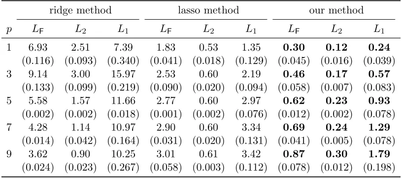
(AbT₁, . . . ,AbT_p)T with regard to different matrix norms (L_F, L₂, and L₁ norms). We conduct 1,000 simulations and compare the averaged performance of three competing methods. The calculated averaged estimation errors are illustrated in Tables 11 and 12. The standard devi-ations of the estimation errors are provided in the parentheses. Here the tuning parameters are selected in the same way as before. Tables 11 and 12 confirms that our method still outperforms the competing two methods.

5.2.3 Synthetic Data: Impact of Transition Matrices’ Spectral Norms

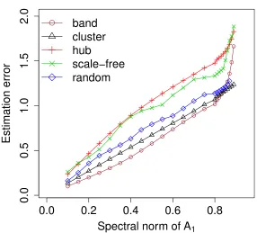
In this section we illustrate the effects of the transition matrices’ spectral norms on esti-mation accuracy. To this end, we study the settings in Section 5.2. More specifically, we set lag p = 1, the dimension d and the sample size T to be d = 50 and T = 100. The transition matrix A1 is created according to different patterns (“band”, “cluster”, “hub”, “scale-free”, and “random”), and then rescaled such thatkA1k2 =κ, whereκis from 0.05 to 0.9. Covariance matrix Σ is set to be of the form (22), and Ψ is accordingly determined by stationary condition. We select the tuning parameters using the cross-validation procedure as before. The estimation errors are then plotted againstκ and shown in Figure 2.

ridge method lasso method our method

p LF L2 L1 LF L2 L1 LF L2 L1

1 6.93 2.50 7.35 1.83 0.52 1.36 0.25 0.11 0.23 (0.012) (0.094) (0.377) (0.039) (0.017) (0.128) (0.014) (0.016) (0.002) 3 9.13 2.89 15.96 2.52 0.59 2.18 0.45 0.18 0.70

(0.129) (0.092) (0.249) (0.085) (0.016) (0.116) (0.023) (0.004) (0.003) 5 5.57 1.57 11.73 2.75 0.61 3.19 0.58 0.23 1.23

(0.000) (0.000) (0.000) (0.000) (0.000) (0.000) (0.000) (0.000) (0.000) 7 4.27 1.14 10.92 2.90 0.60 3.44 0.72 0.31 1.83

(0.010) (0.041) (0.152) (0.026) (0.025) (0.183) (0.077) (0.067) (0.222) 9 3.59 0.90 10.17 2.98 0.61 4.11 0.70 0.30 2.11

(0.026) (0.023) (0.219) (0.061) (0.004) (0.201) (0.000) (0.000) (0.000)

Table 11: Comparison of estimation performance of three methods over 1,000 replications under multiple lag settings. The standard deviations are presented in the paren-theses. Here LF, L2, and L1 represent the Frobenius, L2, and L1 matrix norms respectively. The pattern of the transition matrix is “hub”.

ridge method lasso method our method

p LF L2 L1 LF L2 L1 LF L2 L1

1 6.93 2.51 7.39 1.83 0.53 1.35 0.30 0.12 0.24 (0.116) (0.093) (0.340) (0.041) (0.018) (0.129) (0.045) (0.016) (0.039) 3 9.14 3.00 15.97 2.53 0.60 2.19 0.46 0.17 0.57

(0.133) (0.099) (0.219) (0.090) (0.020) (0.094) (0.058) (0.007) (0.083) 5 5.58 1.57 11.66 2.77 0.60 2.97 0.62 0.23 0.93

(0.002) (0.002) (0.018) (0.001) (0.002) (0.076) (0.012) (0.002) (0.078) 7 4.28 1.14 10.97 2.90 0.60 3.34 0.69 0.24 1.29

(0.014) (0.042) (0.164) (0.031) (0.020) (0.131) (0.041) (0.005) (0.078) 9 3.62 0.90 10.25 3.01 0.61 3.42 0.87 0.30 1.79

(0.024) (0.023) (0.267) (0.058) (0.003) (0.112) (0.078) (0.012) (0.198)

0.0

0.2

0.4

0.6

0.8

0.0

0.5

1.0

1.5

2.0

Estimation Error v.s Spectral Norm of

A

Spectral norm of

A

Estimation error

● ●

● ●

● ●

● ●

● ●

● ●

● ●

● ●●

●● ●

● ●

● ●

●

band

cluster

hub

scale−free

random

Figure 2: Estimation errors of A1 (inL1 norm) plotted against spectral norms ofA1. 5.2.4 Computation Time and Memory Usage

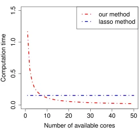
This section is devoted to show the computation time and memory usage of our method. First, we show the advantage of our method in terms of saving the computation time. A major advantage of our method over the two competing methods is that our method can be easily parallelly computed, and hence has the potential to save the computation time. We illustrate this point with a figure and two tables using the computation time as a function of the number of available cores. All experiments are conducted on a 2816-core Westmere/Ivybridge 2.67/2.5GHz Linux server with 17T memory, a cluster system with batch scheduling.

We first focus on the lag p = 1 case. In detail, we set the time series length T = 100 and the dimension d = 50. The transition matrix A1 is created according to the pattern “random”, and then rescaled such thatkA1k2= 0.5. The covariance matrix Σ is generated as in (22), and Ψ is generated by stationary condition. We then solve (11) using parallel computing based on 1 to 50 cores.

Figure 3 shows the computation time. It illustrates that, in terms of saving the com-putation time, under this specific setting, we have: (i) Our method outperforms the ridge method even if we do not parallelly compute it; (ii) When there are no less than 8 cores, our method outperforms the lasso method. Here the ridge method is very slow because it involves calculating the inverse of a large matrix.

0

10

20

30

40

50

0.0

0.5

1.0

1.5

Time Usage v.s # of Available Cores

Number of available cores

Computation time

our method

lasso method

lasso method our method (with # of available cores)

p N/A 1 5 10 20 30 40 50

1 0.260 1.277 0.261 0.132 0.067 0.048 0.033 0.029 2 0.664 2.732 0.553 0.280 0.141 0.098 0.073 0.059 3 1.034 8.945 1.792 0.897 0.455 0.299 0.230 0.181 4 1.538 18.278 3.695 1.844 0.920 0.620 0.466 0.366 5 1.946 35.609 7.130 3.890 1.781 1.189 0.870 0.719

Table 13: A comparison of computation time with increasing number of lagsp: lasso method v.s our method. The computation time for the lasso method does not change with number of available cores. The computation time here is the averaged elapsed time (in seconds) of 100 replicates of a single experiment.

set the time series length T = 100 and the dimension d = 50. The transition matrices

A1, . . . , Ap are created according to the pattern “random”, and then rescaled such that

kAik2 = 0.1 fori = 1, . . . , p. The error covariance matrix Ψ and the covariance matrix Σe are generated in the same way as in Section 5.2.2. With{Ai}p_i=1,Σ, and Ψ determined, wee simulate a time series (X1, . . . , XT)T ∈RT×d according to the model described in (2). We

then solve (11) using parallel computing based on 1 to 50 cores.

Table 13 lists the averaged elapsed time of 100 replicates of one single experiment. Here for each replication, the parameters (A1, . . . , Ap,Ψ,Σ) in the experiment are regenerated.e It illustrates that, in terms of saving the computation time, under this specific setting, we have: (i) When there is only one core, the lasso method outperforms our method. But when there are no less than 20 cores, our method outperforms the lasso method for all lags

p= 1,2,3,4,5; (ii) Asp grows, the advantage of parallel computing will be less significant (The ratio of computation time between our method at the maximum number of available cores and the lasso method tends to increase). We also observe from Table 13 that: (iii) The computation time of our method is approximately increasing quadratically with regard to the lag p, while the computation time of the lasso method is approximately increasing linearly with regard to the lag p.

Similarly, to study the advantage of parallel computing when the dimension d grows, we provide an experiment focusing on models with varying dimensions. We consider the settings where the lengthT = 100, the lagp= 1, and the dimensiondvaries from 10 to 200. The transition matrix A1 is created according to the pattern “random”, and then rescaled such thatkA1k2= 0.5. The covariance matrix Σ is generated as in (22), and Ψ is generated by stationary condition. We then solve (11) using parallel computing based on 1 to 200 cores.

lasso method our method (with # of available cores)

d N/A 1 5 10 20 50 100 200

10 0.022 0.074 0.015 0.008 N/A N/A N/A N/A 20 0.048 0.265 0.055 0.027 0.014 N/A N/A N/A 50 0.153 1.164 0.234 0.120 0.061 0.027 N/A N/A 100 0.468 6.354 1.281 0.649 0.318 0.131 0.067 N/A 200 2.320 21.503 4.304 2.157 1.111 0.448 0.219 0.108

Table 14: A comparison of computation time with increasing dimensiond: lasso method v.s our method. The computation time for the lasso method does not change with number of available cores. The computation time here is the averaged elapsed time (in seconds) of 100 replicates of a single experiment.

Asdgrows, the advantage of parallel computing will be more significant (The ratio between our method at the maximum number of available cores and the lasso method decreases).

Tables 13 and 14 illustrate that, whenpordgrows, the advantage of parallel computing becomes less or more significant respectively. Such results are reasonable because (3.4) can be decomposed to at most dsubproblems in a columnwise way, and solved in parallel. As the dimension dgrows, the maximum number of decomposed subproblems accordingly grows, and hence the gain in parallel computing will be more significant. In comparison, as

p grows (whiledis fixed), the maximum number of subproblems does not grow, and hence the advantage of parallel computing is less significant.

Secondly, we show the memory usage of our method. By converting the time series from VAR(1) to VAR(p) or increasing the dimension d, the memory usage increases. For investigating the memory usage, we conduct an empirical study. Specifically, first, we choose the lagpto be 1,2, . . . ,9, the time series lengthT = 100, and the dimensiond= 50. Transition matrices A1, . . . , Ap are created according to the “random” pattern, and then

rescaled such that kAik2 = 0.1 for i= 1, . . . , p. Ψ is set as Id for simplicity. With {Ai}p_i=1

and Ψ, we simulate a time series (X1, . . . , XT)T ∈ RT×d according to (2) with lagp ≥1.

The first two rows in Table 15 reports the averaged memory usage of 100 replicates of one single experiment in megabytes (Mb). Here for each replication, the parameters in the experiment are regenerated.

Secondly, we choose the lagp= 1, the time series lengthT = 100, the dimensiond= 50, and the transition matrix A1 to be created according to the “random” pattern, and then rescaled such that kA1k2 = 0.1. Ψ is set as Id for simplicity. WithA1 and Ψ, we simulate a time series (X1, . . . , XT)T ∈ RT×d according to (2). The second two rows in Table 15

reports the memory usage.

Lag of model (p) 1 2 3 4 5 6 7 8 9

Mem. Use (Mb) 5.566 8.724 11.862 14.999 18.135 21.272 24.406 27.540 30.673

Dimension (d) 10 20 30 40 50 75 100 150 200

Mem. Use (Mb) 1.649 2.235 3.083 4.194 5.566 10.150 16.390 33.754 57.678

Table 15: Memory usage v.s lag of model and dimension: The result shown below is the averaged memory usage (in Mb) of 100 replicates of one single experiment, with the lagpchanging from 1 to 9 or dimension changing from 10 to 200. The pattern of the transition matrices{Ai}p_i=1 is “random”.

5.3 Real Data

We further compare the three methods on the equity data collected from Yahoo! Finance. The task is to predict the stock prices. We collect the daily closing prices for 91 stocks that are consistently in the S&P 100 index between January 1, 2003 and January 1, 2008. This gives us altogether 1,258 data points, each of which corresponds to the vector of closing prices on a trading day.

We first provide comparison on averaged prediction errors for using different lag p on this data set. Let E = (Et,j) ∈R1258×91 with Et,j denoting the closing price of the stock

j on day t. We screen out all the stocks with low marginal standard deviations and only keep 50 stocks which vary the most. We center the data so that the marginal mean of each time series is zero. The resulting data matrix is denoted by ¯E ∈ _R1258×50_{. We apply the} three methods on ¯E with different lagp changing from 1 to 9. To evaluate the performance of the three methods, for t = 1248, . . . ,1257, we select the data set ¯EJt,∗, where we have

Jt = {j :t−100 ≤j ≤t−1}, as the training set. Then for each p and λ, based on the

training set ¯EJt,∗, we calculate the transition matrix estimates Ab

t

1(p, λ), . . . ,Abt_p(p, λ). We then use the obtained estimates to predict the stock price in dayt. The averaged prediction error for each specific λand pis calculated as

Err(p, λ) = 1 10

10 X

t=1

kE¯t,∗− p

X

k=1 b

At_k(p, λ)T_E¯

t−k,∗k2.

In Table 16, we present the minimized averaged prediction errors minλErr(p, λ) for the

three methods with different lag p. The standard deviations of the prediction errors are presented in the parentheses. Our method outperforms the two competing methods in terms of prediction accuracy.

Secondly, we provide the prediction error on day t= 1258 based on the selected (p, λ) using cross-validation. By observing Table 16, we select the lagp= 1 and the corresponding

lag ridge method lasso method our method

p=1 17.68 (2.49) 15.67 (2.74) 11.88 (3.34)

p=2 15.63 (3.01) 15.69 (2.84) 12.01 (3.41)

p=3 15.17 (3.53) 15.76 (2.83) 12.04 (3.42)

p=4 14.90 (3.69) 15.68 (2.76) 12.02 (3.41)

p=5 14.73 (3.66) 15.62 (2.55) 12.08 (3.29)

p=6 14.58 (3.57) 15.51 (2.58) 12.09 (3.15)

p=7 14.42 (3.49) 15.45 (2.59) 12.21 (3.16)

p=8 14.36 (3.42) 15.40 (2.57) 12.25 (3.16)

p=9 14.20(3.31) 15.28(2.46) 12.24 (3.06)

Table 16: The optimized averaged prediction errors for the three methods on the equity data, under different lags p from 1 to 9. The standard deviations are present in the parentheses. The smallest prediction error within each column is bolded.

6. Discussions

Estimation of the vector autoregressive model is an interesting problem and has been in-vestigated for a long time. This problem is intrinsically linked to the regression problem with multiple responses. Accordingly (penalized) least squares estimates, which has the maximum likelihood interpretation behind it, look like reasonable solutions. However, high dimensionality brings significantly new challenges and viewpoints to this classic problem. In parallel to the Dantzig selector proposed by Candes and Tao (2007) in cracking the or-dinary linear regression model, we advocate borrowing the strength of the linear program in estimating the VAR model. As has been repeatedly stated in the main text, this new formulation brings some advantages over the least square estimates. Moreover, our theo-retical analysis brings new insights into the problem of transition matrix estimation, and we highlight the role ofkA1k2 in evaluating the estimation accuracy of the estimator.

In the main text we do not discuss estimating the covariance matrix Σ and Ψ. Lemma 1 builds the Lmax convergence result for estimating Σ. If we further suppose that the covariance matrix Σ is sparse in some sense, then we can exploit the well developed results in covariance matrix estimation (including “banding”, Bickel and Levina, 2008b, “tapering”, Cai et al., 2010, and “thresholding”, Bickel and Levina, 2008a) to estimate the covariance matrix Σ and establish the consistency result with regard to the matrixL1 and L2 norms. With both Σ and A estimated by some constant estimatorΣ, an estimatorb Ψ of Ψ can beb obtained under the VAR model (with lag one) as

b

Ψ =Σb −AbT₁ΣbAb₁,

and a similar estimator can be built for lagpVAR model using the augmented formulation shown in Equation (4).

assumption in analysis and is adopted by most recent works, for example, Kock and Callot (2015) and Song and Bickel (2011). We notice that there are works in handling unstable VAR models, checking for example Song et al. (2014) and Kock (2012). We would like to explore this problem in the future. Another unexplored region is how to determine the order (lag) of the vector autoregression aside from using the cross-validation approach. There have been results in this area (e.g., Song and Bickel, 2011) and we are also interested in finding whether the linear program can also be exploited in determining the order of the VAR model.

Acknowledgments

We thank the associate editor and three anonymous referees for their helpful comments. Fang’s research is supported by a Google fellowship. Han Liu is grateful for the support of NSF CAREER Award DMS1454377, NSF IIS1408910, NSF IIS1332109, NIH R01MH102339, NIH R01GM083084, and NIH R01HG06841.

Appendix A. Proofs of Main Results

In this section we provide the proofs of the main results in the manuscript.

A.1 Proof of Theorem 1

Before proving the main result in Theorem 1, we first establish several lemmas. In the sequel, because we only focus on the lag 1 autoregressive model, for notation simplicity, in Σi({(Xt)}) we remove {(Xt)} and simply denote the lagicovariance matrix to be Σi.

The following lemma describes theLmax rate of convergence S to Σ. This result gener-alizes the upper bound derived when data are independently generated (see, for example, Bickel and Levina, 2008a).

Lemma 1 Letting S be the marginal sample covariance matrix defined in (7), when T ≥ max(6 logd,1), we have, with probability no smaller than 1−6d−1,

kS−Σkmax≤

16kΣk2maxj(Σjj)

minj(Σjj)(1− kA1k2) (

6 logd

T

1/2 + 2

1

T

1/2)

.

Proof [Proof] For anyj, k∈ {1,2, . . . , d}, we have

P(|Sjk−Σjk|> η) =P

1

T

T

X

t=1

Xtj Xtk−Σjk

> η

!

LettingYt={Xt1(Σ11)−1/2, . . . , Xtd(Σdd)−1/2}Tfort= 1, . . . , T andρjk = Σjk(ΣjjΣkk)−1/2,

we have

P(|Sjk−Σjk|> η) =P

( 1 T T X t=1

YtjYtk−ρjk

> η(ΣjjΣkk)−1/2

) =P ( PT

t=1(Ytj+Ytk)2−

PT

t=1(Ytj−Ytk)2

4T −ρjk

> η(ΣjjΣkk)−1/2

) ≤_P ( 1 T T X t=1

(Ytj+Ytk)2−2(1 +ρjk)

>2η(ΣjjΣkk)−1/2

) +P ( 1 T T X t=1

(Ytj−Ytk)2−2(1−ρjk)

>2η(ΣjjΣkk)−1/2

)

. (23)

Using the property of Gaussian distribution, we have (Y1j+Y1k, . . . , YT j+YT k)T ∼NT(0, Q)

for some positive definite matrixQ. In particular, we have

|Qil|=|Cov(Yij+Yik, Ylj+Ylk)|=|Cov(Yij, Ylj)+Cov(Yij, Ylk)+Cov(Yik, Ylk)+Cov(Yik, Ylj)|

≤ 1

minj(Σjj)

|Cov(Xij, Xlj) + Cov(Xij, Xlk) + Cov(Xik, Xlk) + Cov(Xik, Xlj)|

≤ 4

minj(Σjj)

kΣl−ikmax≤

8kΣk₂kA1k |l−i| 2 minj(Σjj)

,

where the last inequality follows from (3). Therefore, using the matrix norm inequality,

kQk₂ ≤ max 1≤i≤T

T

X

l=1

|Qil| ≤

8kΣk₂

minj(Σjj)(1− kA1k2)

.

Then applying Lemma 3 to (23), we have

P ( 1 T T X t=1

(Ytj+Ytk)2−2(1 +ρjk)

>2η(ΣjjΣkk)−1/2

)

≤2 exp "

−T 2

ηminj(Σjj)(1− kA1k2) 16kΣk₂(ΣjjΣkk)1/2

−2T−1/2

2#

+ 2 exp

−T 2

. (24)

Using a similar argument, we have

P ( 1 T T X t=1

(Ytj−Ytk)2−2(1−ρjk)

>2η(ΣjjΣkk)−1/2

)

≤2 exp "

−T 2

ηminj(Σjj)(1− kA1k2) 16kΣk₂(ΣjjΣkk)1/2

−2T−1/2

2#

+ 2 exp

−T 2

Combining (24) and (25), then applying the union bound, we have

P(kS−Σkmax> η)

≤3d2exp

−T 2

+3d2exp 

−

T

2 (

ηminj(Σjj)(1− kA1k2) 16kΣk2maxj(Σjj)

−2

1

T

−1/2)2 

.

The proof thus completes by choosingη as the described form.

In the next lemma we try to quantify the difference between S1 and Σ1 with respect to the matrixLmaxnorm. Remind that Σ1{(Xt)}is simplified to be Σ1.

Lemma 2 LettingS1 be the lag 1 sample covariance matrix, when T ≥max(6 logd+ 1,2), we have, with probability no smaller than 1−8d−1,

kS1−Σ1kmax≤

32kΣk₂maxj(Σjj)

minj(Σjj)(1− kA1k2) (

3 logd

T

1/2 +

2

T

1/2)

.

Proof [Proof] We have, for any j, k∈ {1,2, . . . , d},

P(|(S1)jk−(Σ1)jk|> η) =P

1

T −1

T−1 X

t=1

XtjX(t+1)k−(Σ1)jk

> η ! .

LettingYt={Xt1(Σ11)−1/2, . . . , Xtd(Σdd)−1/2}T and ρjk = (Σ1)jk(ΣjjΣkk)−1/2, we have

P(|(S1)jk−(Σ1)jk|> η) =P

( 1

T−1

T−1 X

t=1

YtjY(t+1)k−ρjk

> η(ΣjjΣkk)−1/2

) =P "

PT−1

t=1{Ytj+Y(t+1)k}2−

PT−1

t=1 {Ytj−Y(t+1)k}2

4(T−1) −ρjk

> η(ΣjjΣkk)−1/2

# ≤_P "

PT−1

t=1{Ytj+Y(t+1)k}2

T−1 −2(1 +ρjk)

>2η(ΣjjΣkk)−1/2

# +P "

PT−1

t=1 {Ytj−Y(t+1)k}2

T −1 −2(1−ρjk)

>2η(ΣjjΣkk)−1/2

#

. (26)

Using the property of Gaussian distribution, we have {Y1j +Y2k, . . . , Y(T−1)j +YT k}T ∼

NT−1(0, Q),for some positive definite matrixQ. In particular, we have

|Qil|=|Cov{Yij +Y(i+1)k, Ylj +Y(l+1)k}|

=|Cov(Yij, Ylj) + Cov{Yij, Y(l+1)k}+ Cov{Y(i+1)k, Ylj}+ Cov{Y(i+1)k, Y(l+1)k}|

≤ 1

minj(Σjj)

|Cov(Xij, Xlj)+Cov{Xij, X(l+1)k}+Cov{X(i+1)k, Xlj}+Cov{X(i+1)k, X(l+1)j}|

≤ 2kΣl−ikmax+kΣl+1−ikmax+kΣl−1−ikmax minj(Σjj)

≤ kΣk2(2kA1k

|l−i|

2 +kA1k |l+1−i|

2 +kA1k |l−1−i|

2 )

minj(Σjj)

Therefore, using the matrix norm inequality,

kQk2 ≤ max 1≤i≤(T−1)

T−1 X

l=1

|Qil| ≤

8kΣk2

minj(Σjj)(1− kA1k2)

.

Then applying Lemma 3 to (26), we have

P " 1

T −1

T−1 X

t=1

{Ytj+Y(t+1)k}2−2(1 +ρjk)

>2η(ΣjjΣkk)−1/2

# ≤

2 exp "

−(T −1) 2

ηminj(Σjj)(1− kA1k2) 16kΣk₂(ΣjjΣkk)1/2

−2(T −1)−1/2 2#

+2 exp

−T−1 2

. (27)

Using a similar technique, we have

P " 1

T −1

T−1 X

t=1

{Ytj−Y(t+1)k}2−2(1−ρjk)

>2η(ΣjjΣkk)−1/2

# ≤

2 exp "

−(T −1) 2

ηminj(Σjj)(1− kA1k2) 16kΣk2(ΣjjΣkk)1/2

−2(T −1)−1/2 2#

+2 exp

−T−1 2

. (28)

Combining (27) and (28), and applying the union bound across all pairs (j, k), we have

P(kS1−Σ1kmax> η)≤ 4d2exp

"

−(T−1) 2

ηminj(Σjj)(1− kA1k2) 16kΣk₂maxj(Σjj)

−2(T−1)−1/2 2#

+4d2exp

−T−1 2

.

Finally noting that when T ≥3, we have 1/(T−1)< 2/T. The proof thus completes by choosingη as stated.

Using the above two technical lemmas, we can then proceed to the proof of the main results in Theorem 1.

Proof [Proof of Theorem 1] With Lemmas 1 and 2, we proceed to prove Theorem 1. We first denote

ζ1 =

16kΣk₂maxj(Σjj)

minj(Σjj)(1− kA1k2) (

6 logd

T

1/2 + 2

1

T

1/2)

,

ζ2 =

32kΣk₂maxj(Σjj)

minj(Σjj)(1− kA1k)2 (

3 logd

T

1/2 +

2

T

1/2)

.

Using Lemmas 1 and 2, we have, with probability no smaller than 1−14d−1,

We firstly prove that population quantity A1 is a feasible solution to the optimization problem in (10) with probability no smaller than 1−14d−1

kSA1−S1kmax=kSΣ−1Σ1−S1kmax =kSΣ−1ΣT

1 −Σ1+ Σ1−S1kmax

≤ k(SΣ−1−Id)Σ1kmax+kΣ1−S1kmax

≤ k(S−Σ)Σ−1Σ1kmax+ζ2

≤ζ1kA1k1+ζ2

≤λ0.

The last inequality holds by using the condition that d≥8 implies that 1/T ≤logd/(2T). Therefore,A1 is feasible in the optimization equation, by checking the equivalence between (10) and (11), we havekΩbk₁ ≤ kA₁k₁ with probability no smaller than 1−14d−1. We then have

kΩb−A₁k_max=kΩb−Σ−1Σ₁k_max =kΣ−1(ΣΩb −Σ₁)k_max

=kΣ−1(ΣbΩ−S1+S1−Σ1)kmax

=kΣ−1(ΣbΩ−SΩ +b SΩb−S1) + Σ−1(S1−Σ1)kmax

≤ k(Id−Σ−1S)bΩkmax+kΣ−1(SΩb−S₁)k_max+kΣ−1(S₁−Σ₁)k_max ≤ kΣ−1k₁k(Σ−S)bΩk_max+kΣ−1k₁kSΩb−S₁k_max+kΣ−1k₁kS₁−Σ₁k_max ≤ kΣ−1k1(kA1k1ζ1+λ0+ζ2)

= 2λ0kΣ−1k1.

Letλ1 be a threshold level and we define

s1 = max 1≤j≤d

d

X

i=1

min{|(A1)ij|/λ1,1}, Tj ={i:|(A1)ij| ≥λ1}.

We have, with probability no smaller than 1−14d−1, for all j∈ {1, . . . , d}, kΩb∗,j−(A1)∗,jk1 ≤ kΩb_Tc

j,jk1+k(A1)Tjc,jk1+kΩbTj,j−(A1)Tj,jk1

=kΩb∗,jk1− kΩb_Tj,jk₁+k(A₁)_Tc

j,jk1+kΩbTj,j−(A1)Tj,jk1

≤ k(A1)∗,jk1− kΩb_Tj,jk₁+k(A₁)_Tc

j,jk1+kΩbTj,j−(A1)Tj,jk1

≤2k(A1)Tc

j,jk1+ 2kΩbTj,j−(A1)Tj,jk1

≤2k(A1)Tc

j,jk1+ 4λ0kΣ

−1_k 1|Tj|

≤(2λ1+ 4λ0kΣ−1k1)s1.

Suppose maxjPdi=1|(A1)ij|q ≤sand setting λ1 = 2λ0kΣ−1k1, we have

λ1s1= max 1≤j≤d

d

X

i=1

min{|(A1)ij|, λ1} ≤λ1 max 1≤j≤d

d

X

i=1

Therefore, we have

kΩb∗,j−(A1)∗,jk1≤4λ1s1≤4λ1−₁ qs= 4s(2λ0kΣ−1k1)1−q.

Noting that when the lag of the time series p = 1, by definition in (12), we have Ω =b Ab₁. This completes the proof.

A.2 Proof of the Rest Results

Proof [Proof of Corollary 1] Corollary 1 directly follows from Theorem 1, so its proofs is omitted.

Proof [Proof of Corollary 2] Using the generating model described in Equation (2), we have

kXT+1−AbT₁X_Tk∞=k(AT1 −AbT₁)X_T +Z_T+1k∞

≤kAT

1 −AbT₁k∞kXTk∞+kZT+1k∞ =kA1−Ab₁k₁kX_Tk∞+kZT+1k∞ Using Lemma 4 in Appendix B, we have

P(kXTk∞≤(Σmax·αlogd)1/2,kZT+1k∞≤(Ψmax·αlogd)1/2)≥1−2(dα/2−1 p

π/2·αlogd})−1.

This, combined with Theorem 1, gives Equation (20).

Proof [Proof of Corollary 3] Similar as the proof in Corollary 2, we have

kXT+1−A¯T1XTk2=k(AT1 −A¯ T

1)XT +ZT+1k2

≤kA1−A¯1k2kXTk2+kZT+1k2. For any Gaussian random vectorY ∼Nd(0, Q), we have Y =

√

QY0 whereY0 ∼Nd(0, Id).

Using the concentration inequality for Lipschitz functions of standard Gaussian random vector (see, for example, Theorem 3.4 in Massart, 2007), we have

P(|kYk2−EkYk2| ≥t) =P(|k

p

QY0k2−Ek p

QY0k2| ≥t)

≤2 exp

− t

2 2kQk2

. (29)

Here the inequality exploits the fact that for any vectors x, y∈_Rd_,

|kpQxk2− k p

Qyk2| ≤ k p

Q(x−y)k2≤ k p

Qk2kx−yk2,

and accordingly the functionx→ k√Qxk₂ has the Lipschitz norm no greater thanpkQk₂. Using Equation (29), we then have

P(kXTk2 ≤ p

2kΣk2logd+EkXTk2, kZT+1k2≤ p

Finally, we have

(EkYk2)2≤EkYk22 = tr(Q).

Combined with Theorem 1 and the fact thatkA1−A¯1k2 ≤ kA1−A¯1k1, we have the desired result.

Appendix B. Supporting Lemmas

Lemma 3 (Negahban and Wainwright, 2011) Suppose that Y ∼NT(0, Q) is a Gaus-sian random vector. We have, for η >2T−1/2,

P

n

kYk2₂−E(kYk2₂)

>4T ηkQk₂ o

≤2 exp n

−T(η−2T−1/2)2/2 o

+ 2 exp(−T /2).

Proof [Proof] This can be proved by first using the concentration inequality for the Lips-chitz functionskYk₂ of Gaussian random variables Y. Then combining with the result

kYk2

2−E(kYk22)≤(kYk2−EkYk2)·(kYk2+EkYk2), we have the desired concentration inequality.

Lemma 4 Suppose that Z = (Z1, . . . , Zd)T ∈Nd(0, Q) is a Gaussian random vector. Let-ting Qmax:= maxi(Qii), we have

P{kZk∞>(Qmax·αlogd)1/2} ≤

dα/2−1pπ/2·αlogd−1.

Proof [Proof] Simply using the Gaussian tail probability, we have

P(kZk∞> t)≤ d

X

i=1

P(|Zi| ·Q −1/2

ii > t·Q −1/2 ii )≤

d

X

i=1

2 exp(−t2/2Qii)

t·Q−1_ii /2·√2π

≤ 2dexp(−t

2_/2Q max)

t·Q−1max/2·

√ 2π

.

Taking t= (Qmax·αlogd)1/2 into the upper equation, we have the desired result.

References

J. H. Ahlberg and E. N. Nilson. Convergence properties of the spline fit. Journal of the Society for Industrial and Applied Mathematics, 11(1):95–104, 1963.

J. Bento, M. Ibrahimi, and A. Montanari. Learning networks of stochastic differential equations. In Advances in Neural Information Processing Systems (NIPS), pages 172– 180, 2010.