Consistency of the Group Lasso and Multiple Kernel Learning
Francis R. Bach [email protected]
INRIA - WILLOW Project-Team
Laboratoire d’Informatique de l’Ecole Normale Sup´erieure (CNRS/ENS/INRIA UMR 8548) 45, rue d’Ulm, 75230 Paris, France
Editor: Nicolas Vayatis
Abstract
We consider the least-square regression problem with regularization by a block`1-norm, that is, a sum of Euclidean norms over spaces of dimensions larger than one. This problem, referred to as the group Lasso, extends the usual regularization by the`1-norm where all spaces have dimension one, where it is commonly referred to as the Lasso. In this paper, we study the asymptotic group selection consistency of the group Lasso. We derive necessary and sufficient conditions for the consistency of group Lasso under practical assumptions, such as model misspecification. When the linear predictors and Euclidean norms are replaced by functions and reproducing kernel Hilbert norms, the problem is usually referred to as multiple kernel learning and is commonly used for learning from heterogeneous data sources and for non linear variable selection. Using tools from functional analysis, and in particular covariance operators, we extend the consistency results to this infinite dimensional case and also propose an adaptive scheme to obtain a consistent model estimate, even when the necessary condition required for the non adaptive scheme is not satisfied. Keywords: sparsity, regularization, consistency, convex optimization, covariance operators
1. Introduction
Regularization has emerged as a dominant theme in machine learning and statistics. It provides an intuitive and principled tool for learning from high-dimensional data. Regularization by squared Euclidean norms or squared Hilbertian norms has been thoroughly studied in various settings, from approximation theory to statistics, leading to efficient practical algorithms based on linear algebra and very general theoretical consistency results (Tikhonov and Arsenin, 1997; Wahba, 1990; Hastie et al., 2001; Steinwart, 2001; Cucker and Smale, 2002).
In recent years, regularization by non Hilbertian norms has generated considerable interest in linear supervised learning, where the goal is to predict a response as a linear function of covariates; in particular, regularization by the`1-norm (equal to the sum of absolute values), a method com-monly referred to as the Lasso (Tibshirani, 1996; Osborne et al., 2000), allows to perform variable selection. However, regularization by non Hilbertian norms cannot be solved empirically by simple linear algebra and instead leads to general convex optimization problems and much of the early effort has been dedicated to algorithms to solve the optimization problem efficiently. In particular, the Lars algorithm of Efron et al. (2004) allows to find the entire regularization path (i.e., the set of solutions for all values of the regularization parameters) at the cost of a single matrix inversion.
Lin, 2007; Zou, 2006; Wainwright, 2006) have looked precisely at the model consistency of the Lasso, that is, if we know that the data were generated from a sparse loading vector, does the Lasso actually recover it when the number of observed data points grows? In the case of a fixed number of covariates, the Lasso does recover the sparsity pattern if and only if a certain simple condition on the generating covariance matrices is verified (Yuan and Lin, 2007). In particular, in low correlation settings, the Lasso is indeed consistent. However, in presence of strong correlations between relevant variables and irrelevant variables, the Lasso cannot be consistent, shedding light on potential problems of such procedures for variable selection. Adaptive versions where data-dependent weights are added to the `1-norm then allow to keep the consistency in all situations (Zou, 2006).
A related Lasso-type procedure is the group Lasso, where the covariates are assumed to be clustered in groups, and instead of summing the absolute values of each individual loading, the sum of Euclidean norms of the loadings in each group is used. Intuitively, this should drive all the weights in one group to zero together, and thus lead to group selection (Yuan and Lin, 2006). In Section 2, we extend the consistency results of the Lasso to the group Lasso, showing that similar correlation conditions are necessary and sufficient conditions for consistency. Note that we only obtain results in terms of group consistency, with no additional information regarding variable consistency inside each group. Also, when the groups have size one, then we get back similar conditions than for the Lasso. The passage from groups of size one to groups of larger sizes leads however to a slightly weaker result as we can not get a single necessary and sufficient condition (in Section 2.6, we show that the stronger result similar to the Lasso is not true as soon as one group has dimension larger than one). Also, in our proofs, we relax the assumptions usually made for such consistency results, that is, that the model is completely well-specified (conditional expectation of the response which is linear in the covariates and constant conditional variance). In the context of misspecification, which is a common situation when applying methods such as the ones presented in this paper, we simply prove convergence to the best linear predictor (which is assumed to be sparse), both in terms of loading vectors and sparsity patterns.
The group Lasso essentially replaces groups of size one by groups of size larger than one. It is natural in this context to allow the size of each group to grow unbounded, that is, to replace the sum of Euclidean norms by a sum of appropriate Hilbertian norms. When the Hilbert spaces are reproducing kernel Hilbert spaces (RKHS), this procedure turns out to be equivalent to learn the best convex combination of a set of basis positive definite kernels, where each kernel corresponds to one Hilbertian norm used for regularization (Bach et al., 2004a). This framework, referred to as
multiple kernel learning (Bach et al., 2004a), has applications in kernel selection, data fusion from
heterogeneous data sources and non linear variable selection (Lanckriet et al., 2004a). In this latter case, multiple kernel learning can exactly be seen as variable selection in a generalized additive
model (Hastie and Tibshirani, 1990). We extend the consistency results of the group Lasso to this
nonparametric case, by using covariance operators and appropriate notions of functional analysis. These notions allow to carry out the analysis entirely in “primal/input” space, while the algorithm has to work in “dual/feature” space to avoid infinite dimensional optimization. Throughout the paper, we will always go back and forth between primal and dual formulations, primal formulation for analysis and dual formulation for algorithms.
schemes in Section 4 and illustrate our set of results with simulations on synthetic examples in Section 5.
2. Consistency of the Group Lasso
We consider the problem of predicting a response Y ∈Rfrom covariates X ∈Rp, where X has a block structure with m blocks, that is, X = (X1>, . . . ,Xm>)> with each Xj∈Rpj, j=1, . . . ,m, and
∑m
j=1pj=p. Throughout this paper, unless otherwise specified,kakwill denote the Euclidean norm
of a vector a (for all possible dimensions of a, for example, p, n or pj). The only assumptions that
we make on the joint distribution PXY of(X,Y)are the following:
(A1) X and Y have finite fourth order moments:EkXk4<∞andEY4<∞.
(A2) The joint covariance matrixΣX X =EX X>−(EX)(EX)>∈Rp×pis invertible.
(A3) We denote by(w,b)∈Rp×Rany minimizer ofE(Y−X>w−b)2. We assume thatE((Y−
w>X−b)2|X) is almost surely greater than σ2
min>0. We denote by J={j,wj 6=0} the
sparsity pattern of w.1
The assumption (A3) does not state thatE(Y|X)is an affine function of X and that the conditional variance is constant, as it is commonly done in most works dealing with consistency for linear supervised learning. We simply assume that given the best affine predictor of Y given X (defined by
w∈Rpand b∈R), there is still a strictly positive amount of variance in Y . If (A2) is satisfied, then the full loading vector w is uniquely defined and is equal to w=Σ−X X1ΣXY, whereΣXY =E(XY)−
(EX)(EY)∈Rp. Note that throughout this paper, we do include a non regularized constant term b but since we use a square loss it will optimized out in closed form by centering the data. Thus all our consistency statements will be stated only for the loading vector w; corresponding results for b then immediately follow.
We often use the notationε=Y−w>X−b. In terms of covariance matrices, our assumption
(A3) leads to: Σεε|X =E(εε|X)>σ2min and ΣεX =0 (but ε might not in general be independent from X ).
2.1 Applications of Grouped Variables
In this paper, we assume that the groupings of the univariate variables are known and fixed, that is, the group structure is given and we wish to achieve sparsity at the level of groups. This has numerous applications, for example, in speech and signal processing, where groups may represent different frequency bands (McAuley et al., 2005), or bioinformatics (Lanckriet et al., 2004a) and computer vision (Varma and Ray, 2007; Harchaoui and Bach, 2007) where each group may correspond to different data sources or data types. Note that those different data sources are sometimes referred to as views (see, e.g., Zhou and Burges, 2007).
Moreover, we always assume that the number m of groups is fixed and finite. Considering cases where m is allowed to grow with the number of observed data points, in the line of Meinshausen and Yu (2006), is outside the scope of this paper.
2.2 Notations
Throughout this paper, we consider the block covariance matrixΣX X with m2 blocksΣXiXj, i,j=
1, . . . ,m. We refer to the submatrix composed of all blocks indexed by sets I, J asΣXIXJ. Similarly,
our loadings are vectors defined following block structure, w= (w>1, . . . ,w>m)>and we denote by wI
the elements indexed by I. Moreover we denote by 1q the vector inRq with constant components
equal to one, and by Iqthe identity matrix of size q.
2.3 Group Lasso
We consider independent and identically distributed (i.i.d.) data (xi,yi)∈Rp×R, i=1, . . . ,n,
sampled from PXY and the data are given in the form of matrices ¯Y ∈Rn and ¯X ∈Rn×p and we
write ¯X= (X¯1, . . . ,X¯m)where each ¯Xj∈Rn×pj represents the data associated with group j (i.e., the i-th row of ¯Xj is the j-th group variable for xi, while ¯Yi=yi). Throughout this paper, we make the
same i.i.d. assumption; dealing with non identically distributed or dependent data and extending our results in those situations are left for future research.
We use the square loss, that is, 2n1 ∑ni=1(yi−w>xi−b)2=2n1kY¯−X w¯ −b1nk2, and thus consider
the following optimization problem:
min
w∈Rp,b∈R
1
2nkY¯−X w¯ −b1nk 2+λ
n m
∑
j=1
djkwjk,
where d= (d1, . . . ,dm)>∈Rm is a vector of strictly positive fixed weights. Note that
consider-ing weights in the block`1-norm is important in practice as those have an influence regarding the consistency of the estimator (see Section 4 for further details). Since b is not regularized, we can minimize in closed form with respect to b, by setting b= 1
n1
>
n(Y¯−X w¯ ). This leads to the following
reduced optimization problem in w:
min
w∈Rp
1
2ΣˆYY−Σˆ
>
XYw+
1 2w
>Σˆ
X Xw+λn m
∑
j=1
djkwjk, (1)
where ˆΣYY = 1nY¯>ΠnY , ˆ¯ ΣXY = 1nX¯>ΠnY and ˆ¯ ΣX X = 1nX¯>ΠnX are empirical covariance matrices¯
(with the centering matrix Πn defined as Πn=In−1n1n1>n). We denote by ˆw any minimizer of
Eq. (1). We refer to ˆw as the group Lasso estimate.2 Note that with probability tending to one, if (A2) is satisfied (i.e., ifΣX X is invertible), there is a unique minimum.
Problem (1) is a non-differentiable convex optimization problem, for which classical tools from convex optimization (Boyd and Vandenberghe, 2003) lead to the following optimality conditions (see proof by Yuan and Lin, 2006, and in Appendix A.1):
Proposition 1 A vector w∈Rpwith sparsity pattern J=J(w) ={j,wj6=0}is optimal for problem
(1) if and only if
∀j∈Jc, ΣˆXjXw−ΣˆXjY
6λndj, (2)
∀j∈J, ΣˆX
jXw−ΣˆXjY =−wj λndj
kwjk
. (3)
2.4 Algorithms
Efficient exact algorithms exist for the regular Lasso, that is, for the case where all group dimen-sions pj are equal to one. They are based on the piecewise linearity of the set of solutions as a
function of the regularization parameterλn(Efron et al., 2004). For the group Lasso, however, the
path is only piecewise differentiable, and following such a path is not as efficient as for the Lasso. Other algorithms have been designed to solve problem (1) for a single value ofλn, in the original
group Lasso setting (Yuan and Lin, 2006) and in the multiple kernel setting (Bach et al., 2004a,b; Sonnenburg et al., 2006; Rakotomamonjy et al., 2007). In this paper, we study path consistency of the group Lasso and of multiple kernel learning, and in simulations we use the publicly available code for the algorithm of Bach et al. (2004b), that computes an approximate but entire path, by following the piecewise smooth path with predictor-corrector methods.
2.5 Consistency Results
We consider the following two conditions:
max
i∈Jc
1
di
ΣXiXJΣ
−1
XJXJDiag(dj/kwjk)wJ
<1, (4)
max
i∈Jc
1
di
ΣXiXJΣ
−1
XJXJDiag(dj/kwjk)wJ
61, (5)
where Diag(dj/kwjk)denotes the block-diagonal matrix (with block sizes pj) in which each
diag-onal block is equal to dj
kwjkIpj (with Ipj the identity matrix of size pj), and wJ denotes the
concate-nation of the loading vectors indexed by J. Note that the conditions involve the covariance between all active groups Xj, j∈J and all non active groups Xi, i∈Jc.
These are conditions on both the input (through the joint covariance matrix ΣX X) and on the
weight vector w. Note that, when all blocks have size 1, this corresponds to the conditions derived for the Lasso (Zhao and Yu, 2006; Yuan and Lin, 2007; Zou, 2006). Note also the difference between the strong condition (4) and the weak condition (5). For the Lasso, with our assumptions, Yuan and Lin (2007) has shown that the strong condition (4) is necessary and sufficient for path consistency of the Lasso; that is, the path of solutions consistently contains an estimate which is both consistent for the`2-norm (regular consistency) and the`0-norm (consistency of patterns), if and only if condition (4) is satisfied.
In the case of the group Lasso, even with a finite fixed number of groups, our results are not as strong, as we can only get the strict condition as sufficient and the weak condition as necessary. In Section 2.6, we show that this cannot be improved in general. More precisely the following theorem, proved in Appendix B.1, shows that if the condition (4) is satisfied, any regularization parameter that satisfies a certain decay conditions will lead to a consistent estimator; thus the strong condition (4) is sufficient for path consistency:
Theorem 2 Assume (A1-3). If condition (4) is satisfied, then for any sequenceλnsuch thatλn→0
andλnn1/2→+∞, the group Lasso estimate ˆw defined in Eq. (1) converges in probability to w and
the group sparsity pattern J(wˆ) ={j,wˆj6=0}converges in probability to J (i.e.,P(J(wˆ) =J)→1).
Theorem 3 Assume (A1-3). If there exists a (possibly data-dependent) sequence λn such that ˆw
converges to w and J(wˆ)converges to J in probability, then condition (5) is satisfied.
On the one hand, Theorem 2 states that under the “low correlation between variables in J and variables in Jc” condition (4), the group Lasso is indeed consistent. On the other hand, the re-sult (and the similar one for the Lasso) is rather disappointing regarding the applicability of the group Lasso as a practical group selection method, as Theorem 3 states that if the weak correlation condition (5) is not satisfied, we cannot have consistency.
Moreover, this is to be contrasted with a thresholding procedure of the joint least-square esti-mator, which is also consistent with no conditions (but the invertibility ofΣX X), if the threshold is
properly chosen (smaller than the smallest normkwjkfor j∈J or with appropriate decay
condi-tions). However, the Lasso and group Lasso do not have to set such a threshold; moreover, further analysis show that the Lasso has additional advantages over regular regularized least-square pro-cedure (Meinshausen and Yu, 2006), and empirical evidence shows that in the finite sample case, they do perform better (Tibshirani, 1996), in particular in the case where the number m of groups is allowed to grow. In this paper we focus on the extension from uni-dimensional groups to multi-dimensional groups for finite number of groups m and leave the possibility of letting m grow with n for future research.
Finally, by looking carefully at condition (4) and (5), we can see that if we were to increase the weight dj for j∈Jc and decrease the weights otherwise, we could always be consistent: this
however requires the (potentially empirical) knowledge of J and this is exactly the idea behind the adaptive scheme that we present in Section 4. Before looking at these extensions, we discuss in the next Section, qualitative differences between our results and the corresponding ones for the Lasso.
2.6 Refinements of Consistency Conditions
Our current results state that the strict condition (4) is sufficient for joint consistency of the group Lasso, while the weak condition (5) is only necessary. When all groups have dimension one, then the strict condition turns out to be also necessary (Yuan and Lin, 2007).
The main technical reason for those differences is that in dimension one, the set of vectors of unit norm is finite (two possible values), and thus regular squared norm consistency leads to estimates of the signs of the loadings (i.e., their normalized versions ˆwj/kwˆjk) which are ultimately
constant. When groups have size larger than one, then ˆwj/kwˆjkwill not be ultimately constant (just
consistent) and this added dependence on data leads to the following refinement of Theorem 2 (see proof in Appendix B.3):
Theorem 4 Assume (A1-3). Assume the weak condition (5) is satisfied and that for all i∈Jcsuch that d1
i
ΣXiXJΣ
−1
XJXJDiag(dj/kwjk)wJ
=1, we have
∆>Σ
XJXiΣXiXJΣ −1
XJXJDiag
"
dj/kwjk Ipj− wjw>j
w>jwj
!#
∆>0, (6)
with∆=−Σ−1
XJXJDiag(dj/kwjk)wJ. Then for any sequenceλnsuch thatλn→0 andλnn
1/4→+∞,
This theorem is of lower practical significance than Theorem 2 and Theorem 3. It merely shows that the link between strict/weak conditions and sufficient/necessary conditions are in a sense tight (as soon as there exists j∈J such that pj>1, it is easy to exhibit examples where Eq. (6) is or is
not satisfied). The previous theorem does not contradict the fact that condition (4) is necessary for
path-consistency in the Lasso case: indeed, if wjhas dimension one (i.e., pj=1), then Ipj−
wjw>j
w>jwj is
always equal to zero, and thus Eq. (6) is never satisfied. Note that when condition (6) is an equality, we could still refine the condition by using higher orders in the asymptotic expansions presented in Appendix B.3.
We can also further refined the necessary condition results in Theorem 3: as stated in Theorem 3, the group Lasso estimator may be both consistent in terms of norm and sparsity patterns only if the condition (5) is satisfied. However, if we require only the consistent sparsity pattern estimation, then we may allow the convergence of the regularization parameterλnto a strictly positive limitλ0. In this situation, we may consider the following population problem:
min
w∈Rp
1
2(w−w)
>Σ
X X(w−w) +λ0
m
∑
j=1
djkwjk. (7)
If there existsλ0>0 such that the solution has the correct sparsity pattern, then the group Lasso estimate withλn→λ0, will have a consistent sparsity pattern. The following proposition, which
can be proved with standard M-estimation arguments, make this precise:
Proposition 5 Assume (A1-3). Ifλn tends toλ0>0, then the group Lasso estimate ˆw is
sparsity-consistent if and only if the solution of Eq. (7) has the correct sparsity pattern.
Thus, even when condition (5) is not satisfied, we may have consistent estimation of the sparsity pattern but inconsistent estimation of the loading vectors. We provide in Section 5 such examples.
2.7 Probability of Correct Pattern Selection
In this section, we focus on regularization parameters that tend to zero, at the rate n−1/2, that is,
λn=λ0n−1/2 with λ0>0. For this particular setting, we can actually compute the limit of the probability of correct pattern selection (proposition proved in Appendix B.4). Note that in order to obtain a simpler result, we assume constant conditional variance of Y given w>X :
Proposition 6 Assume (A1-3) and var(Y|w>x) =σ2almost surely. Assume moreoverλ
n=λ0n−1/2
withλ0>0. Then, the group Lasso ˆw converges in probability to w and the probability of correct
sparsity pattern selection has the following limit:
P
max
i∈Jc
1
di
σ λ0
ti−ΣXiXJΣ −1
XJXJDiag
dj
kwjk
wJ
61
, (8)
where t is normally distributed with mean zero and covariance matrix ΣXJcXJc|XJ = ΣXJcXJc− ΣXJcXJΣ
−1
XJXJΣXJXJc (which is the conditional covariance matrix of XJc given XJ).
always a positive probability of estimating the correct pattern of groups (see Bach, 2008a, for ap-plication of this result to model consistent estimation of a bootstrapped version of the Lasso, with no consistency condition).
Moreover, additional insights may be gained from Proposition 6, namely in terms of the depen-dence onσ,λ0and the tightness of the consistency conditions. First, whenλ0tends to infinity, then the limit defined in Eq. (8) tends to one if the strict consistency condition (4) is satisfied, and tends to zero if one of the conditions is strictly not met. This corroborates the results of Theorem 2 and 3. Note however, that only an extension of Proposition 6 toλn that may deviate from a n−1/2would
actually lead to a proof of Theorem 2, which is a subject of ongoing research.
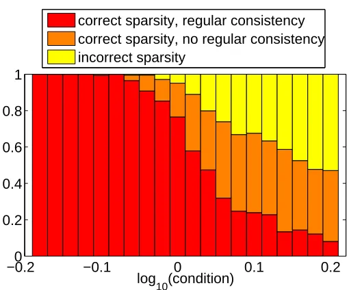
Finally, Eq. (8) shows thatσhas a smoothing effect on the probability of correct pattern selec-tion, that is, if condition (4) is satisfied, then this probability is a decreasing function ofσ(and an increasing function ofλ0). Finally, the stricter the inequality in Eq. (4), the larger the probability of correct rank selection, which is illustrated in Section 5 on synthetic examples.
2.8 Loading Independent Sufficient Condition
Condition (4) depends on the loading vector w and on the sparsity pattern J, which are both a priori unknown. In this section, we consider sufficient conditions that do not depend on the loading vector, but only on the sparsity pattern J and of course on the covariance matrices. The following condition is sufficient for consistency of the group Lasso, for all possible loading vectors w with sparsity pattern J:
C(ΣX X,d,J) =max
i∈Jc ∀j∈Jmax,ku jk=1
1 di
ΣXiXJΣ −1
XJXJDiag(dj)uJ
<1. (9)
As opposed to the Lasso case, C(ΣX X,d,J)cannot be readily computed in closed form, but we
have the following upper bound:
C(ΣX X,d,J)6max i∈Jc
1
di
∑
j∈Jdj
k
∑
∈JΣXiXk
Σ−1
XJXJ
k j ,
where for a matrix M,kMkdenotes its maximal singular value (also known as its spectral norm). This leads to the following sufficient condition for consistency of the group Lasso (which extends the condition of Yuan and Lin, 2007):
max
i∈Jc
1
di
∑
j∈Jdj
k
∑
∈JΣXiXk
Σ−1
XJXJ
k j
<1. (10)
Given a set of weights d, better sufficient conditions than Eq. (10) may be obtained by solving a semidefinite programming problem (Boyd and Vandenberghe, 2003):
Proposition 7 The quantity max
∀j∈J,kujk=1
ΣXiXJΣ
−1
XJXJDiag(dj)uJ
2
is upperbounded by
max
M<0,trMii=1
trMDiag(dj)Σ−XJ1XJΣXJXiΣXiXJΣ −1
XJXJDiag(dj)
where M is a matrix defined by blocks following the block structure ofΣXJXJ. Moreover, the bound is also equal to
min
λ∈Rm,Diag(d
j)Σ−XJXJ1 ΣXJXiΣXiXJΣXJXJ−1 Diag(dj)4Diag(λ)
m
∑
j=1
λj.
Proof We denote M=uu><0. Then if all ujfor j∈J have norm 1, then we have trMj j=1 for
all j∈J. This implies the convex relaxation. The second problem is easily obtained as the convex
dual of the first problem (Boyd and Vandenberghe, 2003).
Note that for the Lasso, the convex bound in Eq. (11) is tight and leads to the bound given above in Eq. (10) (Yuan and Lin, 2007; Wainwright, 2006). For the Lasso, Zhao and Yu (2006) consider several particular patterns of dependencies using Eq. (10). Note that this condition (and not the condition in Eq. 9) is independent from the dimension and thus does not readily lead to rules of thumbs allowing to set the weight dj as a function of the dimension pj; several rules of thumbs have
been suggested, that loosely depend on the dimension on the blocks, in the context of the linear group Lasso (Yuan and Lin, 2006) or multiple kernel learning (Bach et al., 2004b); we argue in this paper, that weights should also depend on the response as well (see Section 4).
2.9 Alternative Formulation of the Group Lasso
Following Bach et al. (2004a), we can instead consider regularization by the square of the block `1-norm:
min
w∈Rp,b∈R
1
2nkY¯−X w¯ −b1nk 2+1
2µn
m
∑
j=1
djkwjk
!2 .
This leads to the same path of solutions, but it is better behaved because each variable which is not zero is still regularized by the squared norm. The alternative version has also two advantages: (a) it has very close links to more general frameworks for learning the kernel matrix from data (Lanckriet et al., 2004b), and (b) it is essential in our proof of consistency in the functional case. We also get the equivalent formulation to Eq. (1), by minimizing in closed form with respect to b, to obtain:
min
w∈Rp
1
2ΣˆYY−ΣˆY Xw+ 1 2w
>Σˆ
X Xw+
1 2µn
m
∑
j=1
djkwjk
!2
. (12)
The following proposition gives the optimality conditions for the convex optimization problem de-fined in Eq. (12) (see proof in Appendix A.2):
Proposition 8 A vector w∈Rp with sparsity pattern J={j, wj6=0}is optimal for problem (12)
if and only if
∀j∈Jc,
ΣˆXjXw−ΣˆXjY
6µndj(∑ni=1dikwik),
∀j∈J, ΣˆXjXw−ΣˆXjY =−µn(∑
n
i=1dikwik)
djwj
kwjk
.
Note the correspondence at the optimum between optimal solutions of the two optimization prob-lems in Eq. (1) and Eq. (12) throughλn=µn(∑ni=1dikwik). As far as consistency results are
paths are the same. For Theorem 2, it does not readily apply. But since the relationship betweenλn
and µn at optimum isλn=µn(∑ni=1dikwik)and that∑ni=1dikwˆikconverges to a constant whenever
ˆ
w is consistent, it does apply as well with minor modifications (in particular, to deal with the case
where J is empty, which requires µn=∞).
3. Covariance Operators and Multiple Kernel Learning
We now extend the previous consistency results to the case of nonparametric estimation, where each group is a potentially infinite dimensional space of functions. Namely, the nonparametric group Lasso aims at estimating a sparse linear combination of functions of separate random variables, and can then be seen as a variable selection method in a generalized additive model (Hastie and Tibshirani, 1990). Moreover, as shown in Section 3.5, the nonparametric group Lasso may also be seen as equivalent to learning a convex combination of kernels, a framework referred to as multiple kernel learning (MKL). In this context it is customary to have a single input space with several kernels (and hence Hilbert spaces) defined on the same input space (Lanckriet et al., 2004b; Bach et al., 2004a).3Our framework accommodates this case as well, but our assumption (A5) regarding the invertibility of the joint correlation operator states that the kernels cannot span Hilbert spaces which intersect.
In this nonparametric context, covariance operators constitute appropriate tools for the statistical analysis and are becoming standard in the theoretical analysis of kernel methods (Fukumizu et al., 2004; Gretton et al., 2005; Fukumizu et al., 2007; Caponnetto and de Vito, 2005). The following section reviews important concepts. For more details, see Baker (1973) and Fukumizu et al. (2004).
3.1 Review of Covariance Operator Theory
In this section, we first consider a single set
X
and a positive definite kernel k :X
×X
→R, as-sociated with the reproducing kernel Hilbert space (RKHS)F
of functions fromX
toR(see, e.g., Sch¨olkopf and Smola 2001 or Berlinet and Thomas-Agnan 2003 for an introduction to RKHS the-ory). The Hilbert space and its dot producth·,·iF are such that for all x∈X
, then k(·,x)∈F
and for all f ∈F
,hk(·,x),fiF = f(x), which leads to the reproducing propertyhk(·,x),k(·,y)iF =k(x,y) for any(x,y)∈X
×X
.3.1.1 COVARIANCEOPERATOR ANDNORMS
Given a random variable X on
X
with bounded second order moment, that is, such thatEk(X,X)<∞, we can define the covariance operator as the bounded linear operatorΣX X from
F
toF
such thatfor all(f,g)∈
F
×F
,hf,ΣX XgiF =cov(f(X),g(X)) =E(f(X)g(X))−(Ef(X))(Eg(X)).
The operatorΣX X is auto-adjoint, non-negative and Hilbert-Schmidt, that is, for any orthonormal
basis(ep)p>1 of
F
, then∑∞p=1kΣX Xepk2F is finite; in this case, the value does not depend on thechosen basis and is referred to as the square of the Hilbert-Schmidt norm. The norm that we use by default in this paper is the operator normkΣX XkF =supf∈F,kfkF=1kΣX XfkF, which is dominated
by the Hilbert-Schmidt norm. Note that in the finite dimensional case where
X
=Rp, p>0 and thekernel is linear, the covariance operator is exactly the covariance matrix, and the Hilbert-Schmidt norm is the Frobenius norm, while the operator norm is the maximum singular value (also referred to as the spectral norm).
The null space of the covariance operator is the space of functions f ∈
F
such that var f(X) =0, that is, such that f is constant on the support of X .3.1.2 EMPIRICALESTIMATORS
Given data xi∈
X
,i=1, . . . ,n, sampled i.i.d. from PX, then the empirical estimate ˆΣX X ofΣX X isdefined such thathf,ΣˆX XgiF is the empirical covariance between f(X)and g(X), which leads to:
ˆ
ΣX X=
1
n
n
∑
i=1
k(·,xi)⊗k(·,xi)−
1
n
n
∑
i=1
k(·,xi)⊗
1
n
n
∑
i=1
k(·,xi),
where u⊗v is the operator defined byhf,(u⊗v)giF =hf,uiFhg,viF. If we further assume that the fourth order moment is finite, that is,Ek(X,X)2<∞, then the estimate is uniformly consistent, that is,kΣˆX X−ΣX XkF =Op(n−1/2)(see Fukumizu et al., 2007, and Appendix C.1), which generalizes
the usual result from finite dimension.4
3.1.3 CROSS-COVARIANCE ANDJOINTCOVARIANCEOPERATORS
Covariance operator theory can be extended to cases with more than one random variables (Baker, 1973). In our situation, we have m input spaces
X
1, . . . ,X
mand m random variables X= (X1, . . . ,Xm)and m RKHS
F
1, . . . ,F
massociated with m kernels k1, . . . ,km.If we assume thatEkj(Xj,Xj)<∞, for all j=1, . . . ,m, then we can naturally define the
cross-covariance operatorsΣXiXj from
F
j toF
isuch that∀(fi,fj)∈F
i×F
j,hfi,ΣXiXjfjiFi =cov(fi(Xi),fj(Xj)) =E(fi(Xi)fj(Xj))−(Efi(Xi))(Efj(Xj)).
These are also Hilbert-Schmidt operators, and if we further assume thatEkj(Xj,Xj)2<∞, for all
j=1, . . . ,m, then the natural empirical estimators converges to the population quantities in
Hilbert-Schmidt and operator norms at rate Op(n−1/2). We can now define a joint block covariance operator
on
F
=F
1× · · · ×F
mfollowing the block structure of covariance matrices in Section 2. As in thefinite dimensional case, it leads to a joint covariance operatorΣX X and we can refer to sub-blocks
asΣXIXJ for the blocks indexed by I and J.
Moreover, we can define the bounded (i.e., with finite operator norm) correlation operators throughΣXiXj =Σ
1/2
XiXiCXiXjΣ
1/2
XjXj (Baker, 1973). Throughout this paper we will make the assumption
that those operators CXiXj are compact for i6= j: compact operators can be characterized as limits
of finite rank operators or as operators that can be diagonalized on a countable basis with spectrum composed of a sequence tending to zero (see, e.g., Brezis, 1980). This implies that the joint operator
CX X, naturally defined on
F
=F
1× · · · ×F
m, is of the form “identity plus compact”. It thus hasa minimum and a maximum eigenvalue which are both between 0 and 1 (Brezis, 1980). If those eigenvalues are strictly greater than zero, then the operator is invertible, as are all the square sub-blocks. Moreover, the joint correlation operator is lower-bounded by a strictly positive constant times the identity operator.
4. A random variable Znis said to be of order Op(an)if for anyη>0, there exists M>0 such that supnP(|Zn|>
3.1.4 TRANSLATIONINVARIANTKERNELS
A particularly interesting ensemble of RKHS in the context of nonparametric estimation is the set of translation invariant kernels defined over
X
=Rp, where p>1, of the form k(x,x0) =q(x0−x) where q is a function onRpwith pointwise nonnegative integrable Fourier transform (which implies that q is continuous). In this case, the associated RKHS isF
={q1/2∗g, g∈L2(Rp)}, where q1/2 denotes the inverse Fourier transform of the square root of the Fourier transform of q and∗denotes the convolution operation, and L2(Rp)denotes the space of square integrable functions. The norm is then equal to
kfk2
F =
Z |F(ω)|2
Q(ω) dω,
where F and Q are the Fourier transforms of f and q (Wahba, 1990; Sch ¨olkopf and Smola, 2001). Functions in the RKHS are functions with appropriately integrable derivatives. In this paper, when using infinite dimensional kernels, we use the Gaussian kernel k(x,x0) =q(x−x0) =exp(−bkx− x0k2), with b>0.
3.1.5 ONE-DIMENSIONAL HILBERTSPACES
In this paper, we also consider real random variables Y andεembedded in the natural Euclidean structure of real numbers (i.e., we consider the linear kernel onR). In this setting the covariance operatorΣXjYfromRto
F
jcan be canonically identified as an element ofF
j. Throughout this paper,we always use this identification.
3.2 Problem Formulation
We assume in this section and in the remaining of the paper that for each j=1, . . . ,m, Xj∈
X
jwhereX
jis any set on which we have a reproducible kernel Hilbert spacesF
j, associated with the positivekernel kj :
X
j×X
j →R. We now make the following assumptions, that extend the assumptions(A1), (A2) and (A3). For each of them, we detail the main implications as well as common natural sufficient conditions. The first two conditions (A4) and (A5) depend solely on the input variables, while the two other ones, (A6) and (A7) consider the relationship between X and Y .
(A4) For each j=1. . . ,m,
F
j is a separable reproducing kernel Hilbert space associated withkernel kj, and the random variables kj(·,Xj) are not constant and have finite fourth-order
moments, that is,Ekj(Xj,Xj)2<∞.
This is a non restrictive assumption in many situations; for example, when (a)
X
j =Rpj andthe kernel function (such as the Gaussian kernel) is bounded, or when (b)
X
j is a compact subset of Rpj and the kernel is any continuous function such as linear or polynomial. This implies notably,as shown in Section 3.1, that we can define covariance, cross-covariance and correlation operators that are all Hilbert-Schmidt (Baker, 1973; Fukumizu et al., 2007) and can all be estimated at rate
Op(n−1/2)in operator norm.
(A5) All cross-correlation operators are compact and the joint correlation operator CX X is
invert-ible.
density pX (and marginal distributions pXi(xi) and pXiXj(xi,xj)) and that the mean square contin-gency between all pairs of variables is finite, that is,
E
p
XiXj(xi,xj) pXi(xi)pXj(xj)
−1
<∞.
The contingency is a measure of statistical dependency (Renyi, 1959), and thus this sufficient con-dition simply states that two variables Xiand Xj cannot be too dependent. In the context of multiple
kernel learning for heterogeneous data fusion, this corresponds to having sources which are hetero-geneous enough. On top of compacity we impose the invertibility of the joint correlation operator; we use this assumption to make sure that the functions f1, . . . ,fmare unique. This ensures the non
existence of any set of functions f1, . . . ,fm in the closures of
F
1, . . . ,F
m, such that var fj(Xj)>0,for all j, and a linear combination is constant on the support of the random variables. In the con-text of generalized additive models, this assumption is referred to as the empty concurvity space assumption (Hastie and Tibshirani, 1990).
(A6) There exists functions f= (f1, . . . ,fm)∈
F
=F
1× · · · ×F
m, b∈R, and a function h of X=(X1, . . . ,Xm) such thatE(Y|X) =∑mj=1fj(Xj) +b+h(X)withEh(X)2<∞,Eh(X) =0 and Eh(X)fj(Xj) =0 for all j=1, . . . ,m and fj ∈
F
j. We assume thatE((Y−f(X)−b)2|X)isalmost surely greater thanσ2min>0 and smaller thanσ2max<∞. We denote by J={j,fj6=0}
the sparsity pattern of f.
This assumption on the conditional expectation of Y given X is not the most general and follows common assumptions in approximation theory (see, e.g., Caponnetto and de Vito, 2005; Cucker and Smale, 2002, and references therein). It allows misspecification, but it essentially requires that the conditional expectation of Y given sums of measurable functions of Xjis attained at functions in the
RKHS, and not merely measurable functions. Dealing with more general assumptions in the line of Ravikumar et al. (2008) requires to consider consistency for norms weaker than the RKHS norms (Caponnetto and de Vito, 2005; Steinwart, 2001), and is left for future research. Note also, that to simplify proofs, we assume a finite upper-boundσ2maxon the residual variance.
(A7) For all j∈ {1, . . . ,m}, there exists gj∈
F
j such that fj =Σ1X/j2Xjgj, that is, each fj is in therange ofΣ1X/j2Xj.
This technical condition, already used by Caponnetto and de Vito (2005), which concerns all RKHS independently, ensures that we obtain consistency for the norm of the RKHS (and not another weaker norm) for the least-squares estimates. Note also that it implies that var fj(Xj)>0, that
is, fj is not constant on the support of Xj.
This assumption might be checked (at least) in two ways; first, if (ep)p>1 is a sequence of eigenfunctions ofΣX X, associated with strictly positive eigenvaluesλp>0, then f is in the range of
ΣX Xif and only if f is constant outside the support of the random variable X and∑p>1λ1phf,epi2is
finite (i.e., the decay of the sequencehf,epi2is strictly faster thanλp).
We also provide another sufficient condition that sheds additional light on this technical con-dition which is always true for finite dimensional Hilbert spaces. For the common situation where
X
j =Rpj, PXj (the marginal distribution of Xj) has a density pXj(xj)with respect to the Lebesguemeasure and the kernel is of the form kj(xj,x0j) =qj(xj−x0j), we have the following proposition
Proposition 9 Assume
X
=Rp and X is a random variable onX
with distribution PX that has a
strictly positive density pX(x)with respect to the Lebesgue measure. Assume k(x,x0) =q(x−x0)for
a function q∈L2(Rp)has an integrable pointwise positive Fourier transform, with associated RKHS
F
. If f can be written as f=q∗g (convolution of q and g) withRRpg(x)dx=0 and
R
Rp g(x)
2
pX(x)dx<∞, then f ∈
F
is in the range of the square rootΣ1X X/2of the covariance operator.The previous proposition gives natural conditions regarding f and pX. Indeed, the condition
R g(x)2
pX(x)dx<∞corresponds to a natural support condition, that is, f should be zero where X has
no mass, otherwise, we will not be able to estimate f ; note the similarity with the usual condition regarding the variance of importance sampling estimation (Br´emaud, 1999). Moreover, f should be even smoother than a regular function in the RKHS (convolution by q instead of the square root of q). Finally, we provide in Appendix E detailed covariance structures for Gaussian kernels with Gaussian variables.
3.2.1 NOTATIONS
Throughout this section, we refer to functions f= (f1, . . . ,fm)∈
F
=F
1× · · ·×F
mand the jointco-variance operatorΣX X. In the following, we always use the norms of the RKHS. When considering
operators, we use the operator norm. We also refer to a subset of f indexed by J through fJ. Note
that the Hilbert normkfJkFJ is equal to kfJkFJ = (∑j∈JkfjkFj)
1/2. Finally, given a nonnegative auto-adjoint operator S, we denote by S1/2its nonnegative autoadjoint square root (Baker, 1973).
3.3 Nonparametric Group Lasso
Given i.i.d data (xi j,yi), i=1, . . . ,n, j=1, . . . ,m, where each xi j ∈
X
j, our goal is to estimateconsistently the functions fj and which of them are zero. We denote by ¯Y ∈Rn the vector of
responses. We consider the following optimization problem:
min
f∈F,b∈R 1 2n
n
∑
i=1
yi− m
∑
j=1
fj(xi j)−b
!2 +µn
2
m
∑
j=1
djkfjkFj
!2 .
By minimizing with respect to b in closed form, we obtain a similar formulation to Eq. (12), where empirical covariance matrices are replaced by empirical covariance operators:
min
f∈F
1
2ΣˆYY− hf,ΣˆXYiF+ 1
2hf,ΣˆX XfiF +
µn
2
m
∑
j=1
djkfjkFj
!2
. (13)
We denote by ˆf any minimizer of Eq. (13), and we refer to it as the nonparametric group Lasso
estimate, or also the multiple kernel learning estimate. By Proposition 13, the previous problem has indeed minimizers, and by Proposition 14 this global minimum is unique with probability tending to one.
Proposition 10 A function f ∈
F
with sparsity pattern J =J(f) ={j, fj 6=0} is optimal forproblem (13) if and only if
∀j∈Jc, ΣˆXjXf−ΣˆXjY
Fj 6µndj(∑
n
i=1dikfikFi), (14)
∀j∈J, ΣˆXjXf−ΣˆXjY =−µn(∑
n
i=1dikfikFi) djfj
kfjkFj
. (15)
A consequence (and in fact the first part of the proof) is that an optimal function f must be in the range of ˆΣXY and ˆΣX X, that is, an optimal f is supported by the data; that is, each fj is a linear
combination of functions kj(·,xi j), i=1, . . . ,n. This is a rather circumvoluted way of presenting the
representer theorem (Wahba, 1990), but this is the easiest for the theoretical analysis of consistency. However, to actually compute the estimate ˆf from data, we need the usual formulation with dual
parameters (see Section 3.5).
Moreover, one important conclusion is that all our optimization problems in spaces of functions can be in fact transcribed into finite-dimensional problems. In particular, all notions from multivari-ate differentiable calculus may be used without particular care regarding the infinite dimension.
3.4 Consistency Results
We consider the following strict and weak conditions, which correspond to condition (4) and (5) in the finite dimensional case:
max
i∈Jc
1
di
Σ
1/2
XiXiCXiXJC −1
XJXJDiag(dj/kfjkFj)gJ
F
i
<1, (16)
max
i∈Jc
1
di
Σ
1/2
XiXiCXiXJC −1
XJXJDiag(dj/kfjkFj)gJ
F
i
61, (17)
where Diag(dj/kfjkFj)denotes the block-diagonal operator with operators
dj
kfjkFjIFj on the diagonal.
Note that this is well-defined because CX Xis invertible and that it reduces to Eq. (4) and Eq. (5) when
the input spaces
X
j, j=1, . . . ,m are of the formRpj and the kernels are linear. The main reasonof rewriting the conditions in terms of correlation operators rather than covariance operators is that correlation operators are invertible by assumption, while covariance operators are not as soon as the Hilbert spaces have infinite dimensions. The following theorems give necessary and sufficient conditions for the path consistency of the nonparametric group Lasso (see proofs in Appendix C.2 and Appendix C.3):
Theorem 11 Assume (A4-7) and that J is not empty. If condition (16) is satisfied, then for any sequence µn such that µn →0 and µnn1/2→+∞, any sequence of nonparametric group Lasso
estimates ˆf converges in probability to f and the sparsity pattern J(fˆ) ={j,fˆj6=0}converges in
probability to J.
Theorem 12 Assume (A4-7) and that J is not empty. If there exists a (possibly data-dependent) sequence µnsuch ˆf converges to f and ˆJ converges to J in probability, then condition (17) is satisfied.
3.5 Multiple Kernel Learning Formulation
Proposition 10 does not readily lead to an algorithm for computing the estimate ˆf . In this section,
following Bach et al. (2004a), we link the group Lasso to the multiple kernel learning framework (Lanckriet et al., 2004b). Problem (13) is an optimization problem on a potentially infinite di-mensional space of functions. However, the following proposition shows that it reduces to a finite dimensional problem that we now precise (see proof in Appendix A.4):
Proposition 13 The dual of problem (13) is
max
α∈Rn,α>1 n=0
− 1
2nkY¯−nµnαk 2− 1
2µn
max
i=1,...,m
α>K
iα
d2
i
, (18)
where (Ki)ab =ki(xa,xb) are the kernel matrices in Rn×n, for i=1, . . . ,m. Moreover, the dual
variableα∈Rnis optimal if and only ifα>1n=0 and there existsη∈Rm+such that∑mj=1ηjd2j =1
and
m
∑
j=1
ηjKj+nµnIn
!
α=Y¯, (19)
∀j∈ {1, . . . ,m}, α
>K
jα
d2j <i=max1,...,m
α>K
iα
di2 ⇒ηj=0. The optimal function may then be written as fj=ηj∑ni=1αikj(·,xi j).
Since the problem in Eq. (18) is strictly convex, there is a unique dual solutionα. Note that Eq. (19) corresponds to the optimality conditions for the least-square problem:
min
f∈F
1
2ΣˆYY− hf,ΣˆXYiF + 1
2hf,ΣˆX XfiF+ 1 2µnj,
∑
ηj>0 kfjk2Fj
ηi
,
whose dual problem is:
max
α∈Rn,α>1 n=0
(
− 1
2nkY¯−nµnαk 2− 1
2µn
α>
∑
mj=1
ηiKi
!
α
) ,
and unique solution isα=Πn(∑mj=1ηjΠnKjΠn+nµnIn)−1ΠnY . That is, the solution of the MKL¯
problem leads to dual parameters α and set of weights η>0 such thatα is the solution to the least-square problem with kernel K=∑mj=1ηjKj. Bach et al. (2004a) has shown in a similar
con-text (hinge loss instead of the square loss) that the optimal ηin Proposition 13 can be obtained as the minimizer of the optimal value of the regularized least-square problem with kernel matrix
∑m
j=1ηjKj, that is:
J(η) = max
α∈Rn,α>1 n=0
(
− 1
2nkY¯−nµnαk 2− 1
2µn
α>
∑
mj=1
ηjKj
!
α
) ,
with respect toη>0 such that∑mj=1ηjd2j =1. This formulation allows to derive probably
this formulation allowsηto be negative, as long as the matrix∑mj=1ηjKj is positive semi-definite.
However, theoretical advantages of such a possibility still remain unclear.
Finally, we state a corollary of Proposition 13 that shows that under our assumptions regarding the correlation operator, we have a unique solution to the nonparametric groups Lasso problem with probability tending to one (see proof in Appendix A.5):
Proposition 14 Assume (A4-5). The problem (13) has a unique solution with probability tending to one.
3.6 Estimation of Correlation Condition (16)
Condition (4) is simple to compute while the nonparametric condition (16) might be hard to check even if all densities are known (we provide however in Section 5 a specific example where we can compute in closed form all covariance operators). The following proposition shows that we can con-sistently estimate the quantities
Σ
1/2
XiXiCXiXJC −1
XJXJDiag(dj/kfjkFj)gJ
F
i
given an i.i.d. sample (see
proof in Appendix C.4):
Proposition 15 Assume (A4-7), andκn→0 andκnn1/2→∞. Let
α=Πn
∑
j∈JΠnKjΠn+nκnIn
!−1
ΠnY¯
and ˆηj = d1j(α>Kjα)1/2. Then, for all i∈Jc, the norm
Σ
1/2
XiXiCXiXJC −1
XJXJDiag(dj/kfjk)gJ
F
i is
consistently estimated by:
(ΠnKiΠn)1/2
∑
j∈JΠnKjΠn+nκnIn
!−1
∑
j∈J 1 ˆ
ηj
ΠnKjΠn
!
α
. (20)
4. Adaptive Group Lasso and Multiple Kernel Learning
In previous sections, we have shown that specific necessary and sufficient conditions are needed for path consistency of the group Lasso and multiple kernel learning. The following procedures, adapted from the adaptive Lasso of Zou (2006), lead to two-step procedures that always achieve both consistency, with no condition such as Eq. (4) or Eq. (16). As before, results are a bit different when groups have finite sizes and groups may have infinite sizes.
4.1 Adaptive Group Lasso
The following theorem extends the similar theorem of Zou (2006), and shows that we can get both
Op(n−1/2)consistency and correct pattern estimation:
Theorem 16 Assume (A1-3) and γ>0. We denote by ˆwLS=Σˆ−1
X XΣˆXY the (unregularized)
least-square estimate. We denote by ˆwAany minimizer of
1
2ΣˆYY−ΣˆY Xw+ 1 2w
>Σˆ
X Xw+
µn
2
m
∑
j=1
kwˆLSj k−γkwjk
If n−1/2µnn−1/2−γ/2, then ˆwAconverges in probability to w, J(wˆA)converges in probability to
J, and n1/2(wˆAJ−wJ)tends in distribution to a normal distribution with mean zero and covariance matrixΣ−X1
JXJ.
This theorem, proved in Appendix D.1, shows that the adaptive group Lasso exhibit all important asymptotic properties, both in terms of errors and selected models. In the nonparametric case, we obtain a weaker result.
4.2 Adaptive Multiple Kernel Learning
We first begin with the consistency of the least-square estimate (see proof in Appendix D.2):
Proposition 17 Assume (A4-7). The unique minimizer ˆfκLSn of
1
2ΣˆYY− hΣˆXY,fiF + 1
2hf,ΣˆX XfiF +
κn
2
m
∑
j=1
kfjk2Fj,
converges in probability to f ifκn→0 andκnn1/2→0. Moreover, we havekfˆκLSn −fkF =Op(κ
1/2
n +
κ−1
n n−1/2).
Since the least-square estimate is consistent and we have an upper bound on its convergence rate, we follow Zou (2006) and use it to defined adaptive weights djfor which we get both sparsity
and regular consistency without any conditions on the value of the correlation operators.
Theorem 18 Assume (A4-7) andγ>1. Let ˆfnLS−1/3 be the least-square estimate with regularization
parameter proportional to n−1/3, as defined in Proposition 17. We denote by ˆfAany minimizer of
1
2ΣˆYY− hΣˆXY,fiF+ 1
2hf,ΣˆX XfiF +
µ0n−1/3 2
m
∑
j=1
k(fˆκLSn)jk−γFjkfjkFj
!2 .
Then ˆfAconverges to f and J(fˆA)converges to J in probability.
Theorem 18 allows to set up a specific vector of weights d. This provides a principled way to define data adaptive weights, that allows to solve (at least theoretically) the potential consistency problems of the usual MKL framework (see Section 5 for illustration on synthetic examples). Note that we have no result concerning the Op(n−1/2) consistency of our procedure (as we have for the
finite dimensional case) and obtaining precise convergence rates is the subject of ongoing research. The following proposition gives the expression for the solution of the least-square problem, necessary for the computation of adaptive weights in Theorem 18.
Proposition 19 The solution of the least-square problem in Proposition 17 is given by
∀j∈ {1, . . . ,m}, fLSj =
n
∑
i=1
αikj(·,xi j)withα=Πn m
∑
j=1
ΠnKjΠn+nκnIn
!−1
ΠnY¯,
with normskFˆLS
j kFj= α
>K
jα
1/2
Other weighting schemes have been suggested, based on various heuristics. A notable one (which we use in simulations) is the normalization of kernel matrices by their trace (Lanckriet et al., 2004b), which leads to dj= (tr ˆΣXjXj)
1/2= (1
ntrΠnKjΠn)
1/2. Bach et al. (2004b) have observed empirically that such normalization might lead to suboptimal solutions and consider weights djthat grow with
the empirical ranks of the kernel matrices. In this paper, we give theoretical arguments that indicate that weights which do depend on the data are more appropriate and work better (see Section 5 for examples).
5. Simulations
In this section, we illustrate the consistency results obtained in this paper with a few simple simula-tions on synthetic examples.
5.1 Groups of Finite Sizes
In the finite dimensional group case, we sampled X∈Rpfrom a normal distribution with zero mean vector and a covariance matrix of size p=8 for m=4 groups of size pj=2, j=1, . . . ,m, generated
as follows: (a) sample an p×p matrix G with independent standard normal distributions, (b) form ΣX X=GG>, (c) for each j∈ {1, . . . ,m}, rescale Xj∈R2so that trΣXjXj =1. We selected Card(J) =
2 groups at random and sampled non zero loading vectors as follows: (a) sample each loading from from independent standard normal distributions, (b) rescale those to unit norm, (c) rescale those by a scaling which is uniform at random between 13 and 1. Finally, we chose a constant noise level of standard deviationσequal to 0.2 times(E(w>X)2)1/2 and sampled Y from a conditional normal distribution with constant variance. The joint distribution on(X,Y)thus defined satisfies with probability one assumptions (A1-3).
For cases when the correlation conditions (4) and (5) were or were not satisfied, we consider two different weighting schemes, that is, different ways of setting the weights djof the block`1-norm:
unit weights (which correspond to the unit trace weighting scheme) and adaptive weights as defined in Section 4.
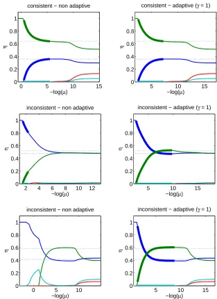
In Figure 1, we plot the regularization paths corresponding to 200 i.i.d. samples, computed by the algorithm of Bach et al. (2004b). We only plot the values of the estimated variables ˆηj,j=
1, . . . ,m for the alternative formulation in Section 3.5, which are proportional tokwˆjkand
normal-ized so that∑mj=1ηˆj=1. We compare them to the population values ηj: both in terms of values,
and in terms of their sparsity pattern (ηjis zero for the weights which are equal to zero). Figure 1
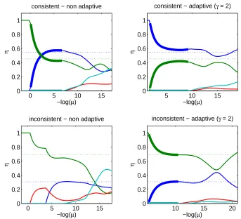
illustrates several of our theoretical results: (a) the top row corresponds to a situation where the strict consistency condition is satisfied and thus we obtain model consistent estimates with also a good estimation of the loading vectors (in the figure, only the behavior of the norms of these loading vectors are represented); (b) the right column corresponds to the adaptive weighting schemes which also always achieve the two type of consistency; (c) in the middle and bottom rows, the consistency condition was not satisfied, and in the bottom row, the condition of Proposition 5, that ensures that we can get model consistent estimates without regular consistency, is met, while it is not in the middle row: as expected, in the bottom row, we get some model consistent estimates but with bad norm estimation.
0 5 10 15 0
0.2 0.4 0.6 0.8 1
−log(µ)
η
consistent − non adaptive
5 10 15
0 0.2 0.4 0.6 0.8 1
−log(µ)
η
consistent − adaptive (γ = 1)
2 4 6 8 10 12
0 0.2 0.4 0.6 0.8 1
−log(µ)
η
inconsistent − non adaptive
5 10 15
0 0.2 0.4 0.6 0.8 1
−log(µ)
η
inconsistent − adaptive (γ = 1)
0 5 10
0 0.2 0.4 0.6 0.8 1
−log(µ)
η
inconsistent − non adaptive
5 10 15
0 0.2 0.4 0.6 0.8 1
−log(µ)
η
inconsistent − adaptive (γ = 1)
Figure 1: Regularization paths for the group Lasso for two weighting schemes (left: non adaptive,
right: adaptive) and three different population densities (top: strict consistency condition
satisfied, middle: weak condition not satisfied, no model consistent estimates, bottom: weak condition not satisfied, some model consistent estimates but without regular con-sistency). For each of the plots, plain curves correspond to values of estimated ˆηj, dotted
curves to population valuesηj, and bold curves to model consistent estimates.
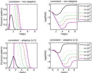
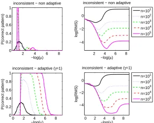
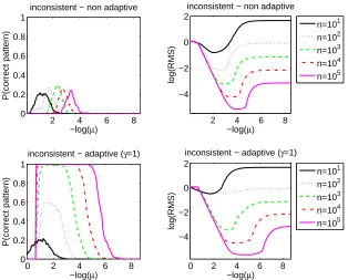
us to estimate both the probability of correct pattern estimationP(J(wˆ) =J)which is considered in Section 2.7, and the logarithm of the expected error logEkwˆ−wk2.