Active Learning by Spherical Subdivision
Falk-Florian Henrich [email protected]
Technische Universit ¨at Berlin Institut f¨ur Mathematik Sekr. MA 8–3
Straße des 17. Juni 136 D-10623 Berlin, Germany
Klaus Obermayer [email protected]
Technische Universit ¨at Berlin Institut f¨ur Informatik FR 2–1, NI
Franklinstraße 28/29 D-10587 Berlin, Germany
Editor: David Cohn
Abstract
We introduce a computationally feasible, “constructive” active learning method for binary classi-fication. The learning algorithm is initially formulated for separable classification problems, for a hyperspherical data space with constant data density, and for great spheres as classifiers. In or-der to reduce computational complexity the version space is restricted to spherical simplices and learning procedes by subdividing the edges of maximal length. We show that this procedure op-timally reduces a tight upper bound on the generalization error. The method is then extended to other separable classification problems using products of spheres as data spaces and isometries in-duced by charts of the sphere. An upper bound is provided for the probability of disagreement between classifiers (hence the generalization error) for non-constant data densities on the sphere. The emphasis of this work lies on providing mathematically exact performance estimates for active learning strategies.
Keywords: active learning, spherical subdivision, error bounds, simplex halving
1. Introduction
Active learning methods seek a solution to inductive learning problems by incorporating the selec-tion of training data into the learning process. In these schemes, the labeling of a data point occurs only after the algorithm has explicitly asked for the corresponding label, and the goal of the “active” data selection is to reach the same accuracy as standard “passive” algorithms—but with less labeled data points. In many practical tasks, the acquisition of unlabeled data can be automated, while the actual labeling must often be done by humans and is therefore time consuming and costly. In these cases, active learning methods—which usually trade labeling costs against the computational burden required for optimal data selection—can be a valuable alternative.
lit-erally “construct” an unlabeled datum and ask the user to provide a label. There is strong empirical evidence for many learning scenarios and for different selection procedures, that active learning methods can reduce the number of labeled training data which are needed to reach a predefined generalization performance (see Balcan et al., 2006; Fine et al., 2002; Freund et al., 1997; Tong and Koller, 2001; Warmuth et al., 2002). In addition, theoretical work has shown that active learning strategies can achieve an exponential reduction of the generalization error with high probability (see Balcan et al., 2006; Freund et al., 1997). In this contribution, we put the emphasis on a mathe-matically rigorous derivation of hard upper bounds for the generalization error. This is in contrast to other studies which give bounds in probability (see Freund et al., 1997) or discuss asymptotic behavior (see Bach, 2007).
We use a geometrical approach to active learning which is based on the concept of a version space (see Mitchell, 1982; Tong and Koller, 2001). Loosely speaking, given a set of predictors and a set of labeled training data, “version space” denotes the set of models whose predictions are consistent with the training data. If a version space can be defined, active learning strategies should evaluate data points which allow the learning machine to maximally reduce the “size” of its version space at every learning step. Some active learning algorithms try to halve the volume of the version space (see Tong and Koller, 2001). In contrast to this, our approach is to reduce the maximal distance between pairs of points that belong to the version space. We prefer distance over volume simply because it is impossible to compute the exact volume of version space in high dimensions. A detailed discussion of this problem can be found at the end of Section 7. For special types of data spaces, our method of maximal length reduction coincides with volume reduction. In this case, we observe a rapid (that is, exponential) progress in learning, as is explicitly shown in Section 4 and Proposition 9 of Section 6 for data which is arbitrarily distributed on an n-dimensional torus.
In the following we will consider the simple case of a separable, binary classification problem. Assuming the knowledge of the data density µ on the data space M, the generalization distance dG(c1,c2)of two classifiers c1,c2: M→ 2:={0,1}is given by the integral
dG(c1,c2):= 1 Vol(M)
Z
D(c1,c2)
ω,
where D(c1,c2):={x∈M|c1(x)6=c2(x)} is the set of points which are classified differently by
the two classifiers, andωdenotes the volume form of M (see Section 2). If we further assume the
labeling of the data to be generated by an unknown classifier c∗: M→ 2, the important question is:
Can we give tight upper bounds on the generalization error dG(c,c∗)of some classifier c, and can we reduce this bound during learning in an optimal way? Inspired by this question, we introduce a constructive active learning algorithm which reduces such a bound by successive subdivisions of the version space on a hypersphere. This then allows us to compute exact and tight generalization error bounds for several classes of data densities. After deriving the bounds for the case of an uniform distribution on the hypersphere, we use the notion of Riemannian isometries to extend the algorithm
and the error bounds to a set of selected data densities on other data spaces including
n. In a second
step, we extend our results to product manifolds in order to obtain sharp error bounds for a larger
set of data densities. Finally, we provide bounds for arbitrary densities on
n, hyperspheres and
products thereof.
The article is organized as follows: After introducing the geometric setup of active learning for binary classification (Section 2), we formulate a learning method for data distributed on the
unit sphere Sn⊂
of separable, binary classification problems using isometries induced by charts of the sphere and products of hyperspheres (Sections 4, 5). This will include perceptrons (that is, linear classifiers
with bias on
n) as a special case. Upper bounds are provided for the generalization error for
non-constant data densities for binary classification problems on the sphere (Section 6) and for linear
classifiers without bias in
n (Section 7). Finally, Section 8 provides an empirical evaluation of
the geometric method. As our focus lies on a theoretical analysis of active learning algorithms, applications of the proposed algorithm to concrete problems have to be of second importance.
2. A Geometric Setup for Active Learning
In the sequel, we will apply some standard constructions from differential geometry. We refer to Appendix B for a quick introduction to the terminology.
Let M be an n-dimensional compact manifold, the data space, equipped with a Riemannian metric g. One might object to this type of data space, since the compactness assumption seems to
rule out the most important instance of data space, the Euclidean space
n. However, this is not
the case, because
n, or any submanifold therein, can be embedded into Sn, the n-sphere, by the
inverse of stereographic projection (see Section 4). Recently, spherical data spaces have received some attention in machine learning (see Lebanon and Lafferty, 2004; Belkin and Niyogi, 2004; Minh et al., 2006).
We assume the existence of an unknown binary classifier c∗: M→ 2:={0,1}and a given set
of labeled data points{(x1,y1), . . . ,(xI,yI))},(xi,yi)∈M× 2, with correct labels, that is, c∗(xi) =
yi. Now, the binary classification problem asks for an approximation c : M→ 2 which minimizes
the generalization error, that is, the probability of misclassification of data points. This can be formalized as follows.
The Riemannian volume form ω which belongs to the metric g is given in local coordinates
x : M⊃U→ nby
ω=pdet(g)dx1∧. . .∧dxn, (1)
where U is some open chart domain in M. We assume that the Riemannian volume formω (see
Equation 1) represents up to a scaling factor Vol(M):=R
Mωthe p.d.f. of the data points x∈M.
This allows us to interpret the probability of disagreement between two classifiers c1,c2as a distance
measure1on the set of all classifiers:
dG(c1,c2):= 1 Vol(M)
Z
D(c1,c2)
ω, (2)
where D(c1,c2):={x∈M|c1(x)6=c2(x)} is called the disagreement area. In these terms, the generalization error of c is given by dG(c,c∗).
3. Subdivisions of the Sphere
In order to be able to compute upper bounds on dG, we need to impose restrictions on the data space
M as well as on the set of classifiers.
1. Depending on the regularity conditions imposed on the classifiers, it might happen that dG(c1,c2) =0 while c16=c2
We start with the following simple setup: Let M=Sn={x∈
n+1| hx,xi=1}, the n-sphere with its canonical Riemannian metric and denote by C the set of hemisphere classifiers
c : Sn→ 2, c(x):=
1 : hx,pi ≥0
0 : hx,pi<0 .
Here, p∈Sn is the center of the hemisphere, and h., .i denotes the Euclidean scalar product in
n+1. This setup implies that the data are uniformly distributed on the sphere. The use of closed
hemispheres as classifiers is appropriate for spherical data, since hemispheres are the direct analog
to half spaces in Euclidean geometry. A simple, yet crucial, observation is the duality C =Sn.
By a slight abuse of notation, we use the symbol c to denote both, the classifier and the center of the hemisphere. Concerning the generalization distance of two classifiers we have the following proposition.
Proposition 1 For hemispheres c1,c2∈C
dG(c1,c2) = 1
πd(c1,c2), where d(c1,c2):=arccos(hc1,c2i)is the geodesic distance on Sn.
Proof The disagreement area D(c1,c2)consists of two congruent lunes on the sphere. The area of
a lune is proportional to its opening angleα=d(c1,c2). Since the total volume of the unit sphere
V :=R
Snωwith respect to its canonical Riemannian metric and volume form is not equal to one, we
have to normalize:
dG(c1,c2) = 1 V
Z
D(c1,c2)
ω= 1
V
α
πV
= 1
πd(c1,c2).
We assume the true classifier c∗ to be some unknown hemisphere. If (x,1) is a labeled data
point, it follows that c∗ is contained in the closed hemisphere around x. Thus, given a labeled
set{(x1,y1), . . . ,(xI,yI))}, c∗ is contained in the intersection V of the corresponding hemispheres.
The version space of a labeled set (see Mitchell, 1982; Tong and Koller, 2001) is defined as the set of classifiers which are consistent with the given labeled data. In our case, the version space coin-cides with the intersection V . Geometrically, V is a convex spherical polytope, a high-dimensional
generalization of a spherical polygon whose edges are segments of great circles and whose(n−1)
-dimensional facets are segments of(n−1)-dimensional great spheres within Sn.
In theory, one can compute the vertices of the version space of any finite labeled set. An iterative algorithm would reduce this polytope by taking intersections with hemispheres corresponding to new data points. Unfortunately, during this process, the number of vertices of the polytope grows exponentially. Thus, the computational costs render its explicit computation impossible even for low dimensions.
Definition 2 (Simplex algorithm)
1. Specify some maximal edge lengthε>0 as termination criterion. Choose a random orthog-onal matrix. Ask for the labels of the n+1 column vectors. This results in a set of admissible classifiers S⊂Snwhich is an equilateral simplex on Sn.
2. Select one of the edges of maximal length of the current simplex S. If its length is less thanε, go to step 7. Otherwise, compute its midpoint m.
3. Compute a unit normal u of the plane in
n+1spanned by m together with all vertices of S which do not belong to the edge through m.
4. Ask for the label l of u. If l=0, replace u by−u.
5. Replace the old simplex S by the part in direction of u, that is, the simplex which has as vertices m as well as all vertices of S with exception of that end point e of the chosen longest edge for whichhu,ei<0.
6. Repeat with step 2.
7. Return the simplex’ center of mass c∈S as the learned classifier.
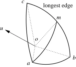
Figure 1 illustrates one iteration of the simplex algorithm on the sphere S2. The “random orthogonal
b m
a o u
c
longest edge
Figure 1: The drawing above shows one iteration of the simplex algorithm for the two-dimensional
case, that is, for spherical triangles on the unit sphere S2. The current version space is
the spherical triangle(a,b,c). The longest edge(b,c) is about to be cut at its midpoint m. Together with the origin o, the vertex a and the point m define a plane in
3 one of
whose unit normal vectors is u∈S2. Depending on the label of u, the new triangle will
be either(a,b,m)or(a,m,c).
matrix” that occurs in step one of the algorithm is meant to be drawn from the uniform distribution on the Lie group
O(n) ={A∈GL(n)|AAt=I}
by evaluating the maximum spherical distance of the chosen classifier to the vertices of the spherical simplex. To be explicit, the following statement holds:
Proposition 3 If S is the current simplex from the simplex algorithm (see Definition 2) with vertices v1, . . . ,vn+1∈Sn, and c∈S some classifier,
dG(c∗,c)≤max
i,j d(vi,vj) =maxi,j arccoshvi,vji.
This bound is tight and attainable if we allow any element of the version space to be the learned classifier. Moreover, if c∈S denotes the center of mass, then
dG(c∗,c)≤max
i d(c,vi) =maxi arccoshc,vii
is a tight and attainable upper bound for the generalization error.
Proof Within a simplex, the maximal distance of two points is realized by pairs of vertices. Now the first inequality follows from proposition 1. If all elements of the simplex are admissible classifiers, the bound is tight. The second inequality follows from the convexity of the simplex.
Clearly, the maximal edge length of the simplex S converges to zero. In Appendix A, we derive
O((n+1)3)as a rough complexity estimate for one iteration of the simplex algorithm (see Definition
2).
Another question concerning the convergence of the algorithm is: How many iterations are needed until the maximum edge length of the initial simplex starts to drop? To this end, we have the following proposition whose proof is given in Appendix A.
Proposition 4 Let S be the initial equilateral simplex from the simplex algorithm (see Definition 2). Let k∈ be the number of steps needed until the maximum of the edge lengths drops. Then
n≤k≤n(n+1)
2 ,
and these bounds are tight and attainable.
4. Extensions by Isometries
We will now extend our results to other data spaces by applying the concept of isometries. The easiest method to obtain isometries from the n-sphere to other data spaces is to consider charts of the sphere together with the induced metric. Being isometries, they preserve the geometry, and any generalization bounds derived for the sphere can be applied without modifications. Combining isometries with the product construction of Section 5, we end up with a large family of data densities
on
nto which our results are directly applicable. In Section 6, we will loosen our preconditions
even further and consider the general case of arbitrary data densities. We begin with the discussion of the stereographic chart of the n-sphere.
Stereographic chart. The stereographic projection
σN: Sn\ {N} →
n,
(x1, . . . ,xn+1)7→
(x1, . . . ,xn)
where N= (0, . . . ,0,1) denotes the north pole, is an isometry of Sn\ {N} to (
n,g), where the
Riemannian metric g is given by
gx(v,w) =
4
(1+kxk2)2hv,wi.
See Figure 2 for an illustration of the two-dimensional case. Hence, we can identify Sn\ {N}with
north pole N of the sphere
point on the sphere
plane of projection (
2) image under projection
Figure 2: The stereographic projection S2\{N} →
2is a diffeomorphism from the sphere with the
north pole removed to the plane. It distorts lengths but preserves angles. If one considers a ray from the north pole to some point on the plane, the stereographic projection will map the intersection point of this ray with the sphere onto its intersection point with the plane.
(
n,g), and the induced Riemannian volume form is
ωx=
2n
(1+kxk2)ndx1∧. . .∧dxn,
where dx1∧. . .∧dxn denotes the Euclidean volume on
n (the determinant). If the given data
density on
n is (up to a constant factor) equal toω, the data can be considered to lie on Sn with
constant density, and our error bounds hold. When viewed under stereographic projection, our spherical classifiers fall in three categories: If the boundary of the hemisphere, which is a great
(n−1)-sphere within Sn, contains the north pole, its projection is a hyperplane through the origin
in
n. The equatorial great sphere{x∈Sn⊂
n+1|x
n+1=0}is projected onto Sn−1⊂
n. All
other great spheres become spheres intersecting Sn−1⊂
northogonally. Hence, any data which is
separable by these classes of hypersurfaces in
nis separable by great spheres on Snand vice versa.
Gnomonic chart. The gnomonic projection
ϕ: Sn⊃ {xn+1>0} →
n,
(x1, . . . ,xn+1)7→
(x1, . . . ,xn)
xn+1 ,
generates on
nthe metric
g= 1
(1+x21+. . .+x2
n)2
s1 −xixj
. .. −xixj sn
point on the sphere
image under projection
plane of projection (
2)
north pole N of the sphere
Figure 3: Illustration of the gnomonic projection for the case S2⊃ {x3>0} →
2. In this case,
we embed
2 at height one into
3, such that it touches the sphere at the north pole.
Rays are sent from the center of the sphere. Their intersection points with the sphere are mapped to the corresponding intersection points with the plane. The gnomonic projection distorts lengths as well as angles, but maps great circles to straight lines.
where we have used the abbreviation si:=1+x21+. . .+x2n−x2i. Figure 3 illustrates the gnomonic
projection in two dimensions. As was the case with the stereographic chart, gnomonic projection is
an isometry from the upper half-sphere to(
n,g). Using Equation 1, we have for x
2=. . .=xn=0
p
det(g) = 1
(1+x21)n+21 .
Since the scaling function of the volume formωhas to be rotationally symmetric, it follows that
ωx=
1
(1+kxk2)n+21
dx1∧. . .∧dxn. (3)
Note that our separating great spheres are projected to affine hyperplanes in
n. Therefore, the
classical approach to the binary classification problem using linear classifiers with bias can be considered a special case of our spherical setup. More precisely, the strict error bounds derived for
our algorithm apply to linear classifiers with bias on
n if and only if the data density on
n is
given by Equation 3. For an analysis that applies to a greater variety of densities we refer to Section 6.
As a byproduct, formula 3 also clarifies the arguments given in the proof of Theorem 4 of Freund et al. (1997) which estimates the information gain of queries made by the Query by Committee algorithm. In the proof, the scaling factor of the volume form of the gnomonic chart is estimated using infinitesimals. The explicit formula for the volume form given above makes this more lucid.
5. Products of Spheres
building blocks for data manifolds and data densities which later can be combined to produce more sophisticated examples. We consider product data manifolds of the type
(M,g) = (Sn1,g1)×. . .×(Snk,gk), (4) where each factor(Snj,gj)is a unit sphere of dimension nj with its standard metric gj. For a point
x= (x1, . . . ,xk)∈M and tangent vectors X = (X1, . . . ,Xk),Y= (Y1, . . . ,Yk)∈TxM we have
gx(X,Y) = k
∑
j=1
gxjj(Xj,Yj).
The Riemannian volume form of the product is given in local coordinates by
ω=
k
∏
j=1
q
det(gj) = k ^
j=1
ωj,
where ωj denotes the volume form of the jth factor. On the product manifold M, we consider
classifiers which are products of hemispheres, that is, C=C1×. . .×Ck, where the Cj=Snj are the
individual sets of hemispheres defined in Section 3 and a classifier c∈C is given by
c : M→ 2, c(x):=
1 : hx,cji ≥0∀j
0 : otherwise .
Due to the simplicity of the product structure, we arrive at the following formula for the generaliza-tion metric:
Proposition 5 For products of hemispheres c1,c2∈C,
dG(c1,c2) = 1
2k−1 1−
1
πk k
∏
j=1
(π−dj(c1j,c2j)),
!
where dj is the geodesic distance on Snj.
Proof Since each component of a classifier is a hemisphere,
Vol(c1j∩c2j) =Vol(Snj)π−dj(c 1
j,c2j)
2π .
Furthermore, the volume of a product of such hemispheres is given by
Vol(c1) =
k
∏
j=1
Vol(c1j) =
k
∏
j=1
Vol(Snj)
2 =
Vol(M)
2k .
Inserting this into
Definition 6 (Extended simplex algorithm)
1. Specify some maximal edge lengthε>0 as termination criterion. For each factor Snj, create an initial simplex using a random orthogonal matrix whose columns are interpreted as a basis for
nj+1. This results in a product S of equilateral simplices.
2. Find one of the edges of maximal length of each factor of the current simplex product S. If all the respective lengths are less than ε, go to step 7. Otherwise, compute the midpoints m1, . . . ,mk.
3. Compute the corresponding unit normals uj.
4. Ask for the labels lj of uj. If lj=0, replace ujby−uj.
5. Replace the old simplex product S by the product of the parts in direction of uj.
6. Repeat with step 2.
7. For each factor, compute its center of mass cj, and return (c1, . . . ,ck)∈S as the learned
classifier.
In parallel to the case of a single sphere, the minimization of maximal edge lengths forces convergence. Note, that if k denotes the number of factors in the product of spheres, then k training points are needed to carry out one iteration of the algorithm. The worst case generalization error after each step is bounded as follows.
Proposition 7 If S is the current product simplex from the extended simplex algorithm (see Defini-tion 6) with maximal edge lengths d1, . . . ,dkof its factors, and c∈S some classifier,
dG(c∗,c)≤ 1
2k−1 1−
1
πk k
∏
j=1
(π−dj)
!
.
This bound is tight and attainable if we allow any element of the version space to be the learned classifier.
Proof In analogy to the case of a single sphere, this follows from proposition 5.
The complexity estimate for one iteration of the extended simplex algorithm is
O((n1+1)3+. . .+ (nk+1)3).
Here, n1, . . . ,nk denote the dimensions of the k individual factors of the product data space. This
Products combined with isometries. We now apply the isometries discussed in Section 4 to product manifolds. For each factor in Equation 4, we may choose one of stereographic or gnomonic projection.
Mn1+...+nk= Sn1 ×. . .× Snk, f1↓ . . . ↓ fk
n1+...+nk=
n1 ×. . .×
nk.
This results in product densities on
n=
n1+...+nk, represented by the volume form
ω=
k
∏
j=1
ωj
with factorsωjgiven by either
ωj
x=
2nj
(1+kxk2)njdx1∧. . .∧dxnj
(stereographic projection) or
ωj
x=
1
(1+kxk2)n j2+1
dx1∧. . .∧dxnj
(gnomonic projection). Similarly, the projected separating hypersurfaces are products of the indi-vidual projections. One could now go on to produce many more families of compatible densities by working with different charts, but instead we turn our attention to an important special case.
The n-torus. A particular case is the gnomonic projection of the n-torus
Tn=S|1×. . .{z×S}1
n factors ,
which yields a scaled version of the Cauchy distribution on
n:
ωx=
n
∏
i=1 1
1+x2idx1∧. . .∧dxn.
Here, we take S1 to be the unit circle which results in Tnhaving total mass (2π)n. Since there is
one circle S1per axis, the projected classifiers are axis parallel corners in
n. One iteration of the
algorithm consumes n labeled data points, because Tn is made up of n individual factors. At each
step of the extended simplex algorithm, the version space is a hypercube of equal edge length l. Therefore, we do not need to compare edge lengths. One step results in halving all the edges, and
the volume is divided by 2n. Hence, if Videnotes the volume after i iterations, we have
Vi=
π
2in.
In analogy, the maximal generalization error Giof the center of mass classifier after i steps is given
by
Gi=
√nπ
2i .
6. Aspherical Data Manifolds
Up to now, our methods apply only to such data manifolds which are isometric to products of subsets of unit spheres. We now loosen this assumption by looking at all oriented Riemannian data
manifolds M which admit an orientation preserving2diffeomorphism
Φ: M→Sn,
that is, Φ is a smooth bijective map which has a smooth inverse. The Riemannian volume form
belonging to the metric g on M induces a volume formωeon Snwhich, in general, is not equal to the
spherical volumeω. More precisely,
e
ω= fω
with some smooth positive scaling function f : Sn→
+. Note that all volume forms (or smooth
positive densities) on Sncan be written in this form. This results in the formula
dG(c1,c2):= 1
f
Vol(Sn) Z
D(c1,c2) fω
for the generalization metric. An illustation of a non-uniform density on the sphere is given in Figure 4 in Section 8 where the reader also finds empirical results for this case.
Concerning the set of admissible classifiers, let us keep the assumption that theΦ-image of the
data is separable by hemisphere classifiers. If we know that the true classifier c∗lies in some subset
S⊂Snthe worst case generalization error of some classifier c∈S is bounded from above by
dG(c,c∗)≤sup
e
c∈S
dG(ec,c∗).
Therefore, the simplex algorithm (see Definition 2) will still converge, as it reduces an upper bound of the generalization error. Its rate of convergence will depend on the properties of the density.
Nevertheless, we can force a simple upper bound by assuming the deviation of the induced volume form from spherical volume to be small:
sup
x∈Sn|
1−f(x)|<ε.
This implies
Proposition 8 Letωbe the canonical volume form of Sn. Denote by dGethe generalization distance induced by the scaled volume form ωe = fω where f : Sn→
+ is some positive smooth scaling
function. If supx∈Sn|1−f(x)|<εfor someε>0 then
dGe(c1,c2)≤(1+ε)Vol(S
n)
πVolf(Sn) d(c1,c2),
where d is the canonical geodesic distance of Sn. In this formula, Vol(Sn):=R
SnωandVolf(Sn):= R
Snωedenote the volumina of Snwith respect toωandωe:= fω.
Proof Using the definition of the generalization distance in Equation 2 and applying proposition 1, we compute
dGe(c1,c2) = 1
f
Vol(Sn) Z
D(c1,c2) fω
≤ 1
f
Vol(Sn) Z
D(c1,c2)
(1+ε)ω
=(1+ε)Vol(S
n)
f
Vol(Sn) d
G(c1,c2)
=(1+ε)Vol(S
n)
πVolf(Sn) d(c1,c2).
Inserting the above upper bound into proposition 3 we obtain
Proposition 9 Let S be the current simplex from the simplex algorithm (see Definition 2) with ver-tices v1, . . . ,vn+1∈Sn, and c∈S⊂Snan arbitrary classifier, not necessarily the center of mass. If c∗∈Sndenotes the unknown true classifier, the generalization error of c is bounded by
dGe(c,c∗)≤(1+ε)Vol(S
n)
πVolf(Sn) maxi,j d(vi,vj),
where d(vi,vj)denotes the spherical distance of the vertices.
The usefulness of the above proposition depends on how much the scaled volume form fωdeviates
from the canonical spherical volumeω. In the case of the n-torus, the same arguments as given at
the end of Section 4 yield an exponential decrease of the volume of the version space as well as of the upper bound for the generalization error—regardless of the data density under consideration.
The only difference is the newly introduced constantεwhich may affect the absolute rate but not
the functional form of convergence.
7. Linear Classifiers without Bias
We now return to the case of linear classifiers on the Euclidean space
nwhich commonly appear
in the machine learning literature. The corresponding separating hypersurfaces are linear subspaces,
that is, hyperplanes through the origin, of
n.
Consider the data space M=
n. Then, the set C of linear classifiers without bias consists of
maps
c : n
→ 2, c(x):=
1 : hx,pi ≥0
0 : hx,pi<0 ,
where p∈Snis the unit normal vector of an oriented(n−1)-dimensional plane through the origin.
Therefore, we can identify C with the unit n-sphere, C=Sn. In the following, we use c to denote
Consider some data density f :
n →
. Since the origin is always classified as +1 by all
classifiers we may remove it from the data space, and the remaining data space is given by
M= n
\ {0}.
Using polar coordinates(s,r), we can write M as the product3 M=Sn−1×
+, s= x
kxk,r=kxk.
For a given s∈Sn−1, we will call the subset Fs:={(s,r)|r>0}the fiber over s. Since the data
is assumed to be separable by at least one element of C any two points belonging to the same fiber have the same label.
The area D(c1,c2)of disagreement between two classifiers c1,c2is given by
D(c1,c2) ={(s,r)∈M| hc1,rsihc2,rsi<0}={(s,r)∈M| hc1,sihc2,si<0}. The generalization distance is given by
dG(c1,c2) =
Z
D(c1,c2) f dx=
Z
{s∈Sn−1|Fs⊂D(c 1,c2)}
Z
Fs
f(s, .)dr
ds, (5)
where dx, dr, ds denote the canonical volume forms on
n, F
s, and Sn−1. It may happen that
different fibers Fshave different mass in the sense that
Sn−1→ , s7→
Z
Fs
f(s, .)dr
is a non-constant function. If we rule out this case we end up with the following proposition:
Proposition 10 The generalization distance of any two linear classifiers c1,c2is given by
dG(c1,c2) =λ
πd(c1,c2),
where d(c1,c2) =arccoshc1,c2iis the geodesic distance on Sn, if and only if the fiber mass is equal to a positive constant,
Z
Fs
f(s, .)dr=λ>0 ∀s∈Sn.
Proof This follows by applying proposition 1 to Equation 5.
The precondition of proposition 10 does not assume that the density f is rotationally invariant
on
n+1. Instead, it assumes the accumulated density to be invariant on the sphere. Linear
classifi-cation problems on non-constant densities which fulfill this condition map to classificlassifi-cation problems with hemisphere classifiers for the uniform density on the sphere. Consequently, all results derived for the spherical simplex algorithm (see Definition 2) apply, including the hard upper bounds on the generalization error. In particular, we deduce the following result from Proposition 3
Proposition 11 If S is the current simplex from the simplex algorithm (see Definition 2) with ver-tices v1, . . . ,vn+1∈Sn, c∗denotes the unknown true classifier and c∈S an arbitrary classifier,
dG(c∗,c)≤λmax
i,j d(vi,vj) =λmaxi,j arccoshvi,vji.
As in Proposition 10,λ>0 denotes the fiber mass. This bound is tight and attainable if we allow any element of the version space to be the learned classifier. Moreover, if c∈S denotes the center of mass, then
dG(c∗,c)≤λmax
i d(c,vi) =λmaxi arccoshc,vii.
is a tight and attainable upper bound for the generalization error.
Relation to SVM methods. Proposition 10 also sheds new light on some active learning strategies that use Support Vector Machines (SVM). A SVM classifier can be interpreted as an approximation
of the center of the largest inscribable hypersphere of the version space on Sn−1 (see Herbrich,
2002). Let us denote this center by p∗∈V ⊂Sn−1, where V ⊂Sn−1is the version space (a spherical polytope, see Section 3) on the hypersphere.
Tong and Koller (2001) argue that, despite its dependence on the particular shape of the version space, the center of the maximal inscribable hypersphere often lies close to “the center of the version space”. Motivated by these insights, they propose the following pool-based strategy for selecting
an unlabeled data point x∈Sn−1to be labeled: Choose x such that the (spherical) distance from the
(n−2)-dimensional great sphere
X :={s∈Sn−1| hx,si=0}
to p∗is minimal. After the data point x is labeled, the version space will be cut into two pieces along
the great sphere X⊂Sn−1. The goal of this strategy is to reduce the volume of the spherical polytope
V as quickly as possible. Similar strategies can be found in Warmuth et al. (2002). Up to now, a closed formula for the volume of a n-spherical simplex is not known, not to speak of polytopes, hence, there is no way of computing the exact volume of a version space on a hypersphere. We refer to Milnor (1994) for a detailed discussion of this topic. Nevertheless, Monte-Carlo methods can be applied to obtain volume estimates.
Proposition 10 can now be applied. The SVM algorithm works with the Euclidean scalar product
on
n, and therefore implicitly assumes the canonical Riemannian metric and volume form on the
unit sphere. Proposition 10 tells us that the SVM approximation is theoretically justified if and only if the given data density induces (up to a constant factor) the uniform density on the sphere.
8. Experimental Results
The following results were obtained from a C++ implementation of the simplex algorithm (see Definition 2). The numerically most sensitive operation of the algorithm is the computation of a
normal vector u∈Sn to the hyperplane H⊂
n+1 whose intersection I=H∩Sn with Sn cuts the
current simplex S into two pieces. In higher dimensions, say n>50,
Z
becomes very small even for small valuesδ>0.4 This means, nearly all the mass of Snis
concen-trated within a thin tube of radiusδaround I, which makes it hard to compute normal vectors. We
avoid numerical problems by using the following procedure:
1. Select the basis of H given by the midpoint of the longest edge and all vertices of the simplex excluding the end points of the longest edge. Construct a corresponding orthonormal basis using the modified Gram-Schmidt algorithm (see Meyer, 2000).
2. Choose random points x∈Snuntil the projected lengthp∑ihx,hii, where hiare the
orthonor-mal basis vectors of H, is less than a given constantε<1.
3. Use x to construct a unit vector which is orthogonal to all basis vectors hi.
In order to test the performance of the simplex algorithm on spheres of different dimensions a series of numerical experiments was conducted, where the following quantities were measured.
Maximal edge length: If(v1, . . . ,vn+1)denote the vertices of the current simplex S of the simplex algorithm, the maximal edge length
max
i,j d(v1,vj)
is an upper bound on the generalization error, regardless which point of the simplex is chosen as the learned classifier.
Maximal distance from center of mass: Let c∈S denote the center of mass of S. Then the maxi-mal distance between c and any other classifier from S is given by
max
i d(c,vi).
This yields a tight upper bound on the generalization error if we choose the center of mass as the learned classifier.
Approximate generalization error for the center of mass classifier c: We estimated the general-ization error of c using the empirical average of the individual errors for 50,000 randomly
se-lected “test” data points. Test data were sampled(i)from a uniform density on the sphere and
(ii)from an aspherical density with two distinct “clusters” at opposite poles. The aspherical
density was constructed by mapping the uniform distribution from an open parameter cuboid onto the sphere using n-spherical coordinates.
Figure 4 illustrates the relation between a sample drawn from this density on the sphere S2
and its stereographic projection onto the plane
2. Densities of this kind are typical for
binary classification problems. Any density with two peaks at p1,p2∈
n can be identified
with a density on Sn with peaks at opposite poles: Firstly, we apply a translation to move
the midpoint of the line p1p2to the origin. Then we use a rotation to place p1,p2on the
x1-axis. After a scaling, p1= (−1,0, . . . ,0)and p2= (+1,0, . . . ,0). Now inverse stereographic projection will map the peaks onto opposite poles.
Figure 4: A data sample from a density with two peaks on
2(left) and S2(right). The data points
on the plane are the stereographic projections of the points on the sphere. On S2, the two
peaks are located at opposite poles.
The above quantities were computed for each step of the simplex algorithm. Averages and variances
were calculated for 1,000 simulations, and averages were normalized to lie within the interval[0,1].
For every simulation, a true classifier was drawn from the uniform distribution on the sphere.
Fig-ures 5 and 6 show the resulting learning curves for the spheres S9⊂
10, S29⊂
30,S49⊂
50, and S79⊂
80. The average maximal edge length as a function of the number of selected training data
!
"#
$
%& '( %)
*
$
$!
$
+ ,+ -+ .+ /+ 0++
0+12 +3++40 +43+40 +30
56789:;<=:>?5?5@A;?5=B><=9:?5?=?>C?D>=?;5 EF
GH
IJK LM JN
O
I
IF
I
P QP RSP RTP SUP VPP
PWPP4R P4WP4R PWR
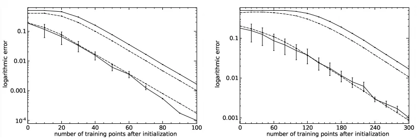
Figure 5: Learning curves on S9⊂
10(left) and on S29⊂
30(right). The figures show the average
maximal edge length (upper solid line), the average maximal distance from the simplex’s center of mass (upper dashed line), and the average approximate generalization errors for the uniform (lower dashed line) and aspherical (lower solid line) data densities as a function of the number of selected training examples. Error bars indicate variances, however, only the approximate generalization error for the aspherical data density shows
large fluctuations between simulation runs. Proposition 4 yields the bounds 9≤k9≤45
and 29≤k29≤435 for the number k of steps needed before the maximal edge length
!
"#
$
%& '( %)
*
$
$!
$
+ ,++ -++ .++ /++ 0++
+1++2, +21+2, +1,
3456789:;8<=3=3>?9=3;@<:;78=3=;=<A=B<;=93 CD
EF
G
HI
JK HL
M
G
GD
G
N ONN PNN QNN RNN SNNN
NTNN2S N2TN2S NTS
Figure 6: Learning curves on S49 ⊂
50 (left) and S79 ⊂
80 (right). For details see legend of
Figure 5. Proposition 4 yields the bounds 49≤k49≤1225 and 79≤k79≤3160 for the
number k of steps needed before the maximal edge length starts to drop on S49and S79.
shows an initial plateau, until the values begin to decrease in an approximately exponential fashion. The length of the plateau increases with the dimensionality of the sphere and is a direct result of Proposition 4. The average maximal distance from the center of mass rises initially (see Figure 7 for a magnified version of the initial segment of the learning curve), until a sudden drop occurs, again followed by a roughly exponential decrease. This can be explained as follows. The simplex algorithm is initialized with an equilateral simplex. During the first learning steps, the center of mass moves towards those vertices whose adjacent edges are cut already. This results in a slight increase of the maximal distance of the vertices from the center of mass. The simplex becomes a “thin pyramid” with small base, and the following drop in the plots then corresponds to a cut of a line connecting the apex to the base. The ratio between the edges connecting the apex to the base
and the edges which are contained within the base is given by n−21, where n is the dimensionality
of the sphere. Since this number tends to zero for n→∞the sudden drop disappears in higher
dimensions.
UVWXY2Z[\^]_Y2Z`_][2Ua
bc
c
dc
e fe ge he ie je
e
ekf ekg ekh eki ekj
Figure 7: Initial learning curves on S9⊂
10(see Figure 5, left), now plotted on a linear scale. For
If the data is drawn from the spherical distribution, the approximate generalization error changes smoothly with the number of selected training data, and its variance is very small. For data dis-tributed according to the aspherical (two cluster) density, the average approximate generalization error is similar, but the variance increases dramatically. Nevertheless, the numerical experiments show that the spherical simplex algorithm performs well even in the case of non-uniform densities.
Experimental results on product manifolds. So far, we restricted the experiments to single spheres instead of products, because the simulation of the extended simplex algorithm on
M=Sn1×. . .×Snk,
is equivalent to the parallel execution of several copies of the basic algorithm. Nevertheless, it might
be interesting to consider the special case of the n-torus Tn(see Section 5):
Tn=S1×. . .×S1
| {z }
n factors .
The product structure of the torus reflects the fact that data is distributed independently on each
factor. For the standard product density on Tn, volume and distances can be computed explicitly.
Therefore, we consider only the non-uniform case. We consider a von Mises density (see Devroye, 1986) on the unit circle:
f : S1= /2π→ , f(x) =
exp(κcos(x−µ)) 2πI0(κ)
.
with center µ∈[0,2π]and widthκ≥0. The symbol I0in the equation above denotes the modified
Bessel function of the first kind of order zero. A technique for simulating the von Mises distribution can be found in Best and Fisher (1979). In order to obtain a density with two peaks on opposite
poles of the circle, we superimpose two copies of f with µ=0 and µ=π. This construction is
applied to every factor S1of the torus Tn=S1×. . .×S1.
We implemented the extended simplex algorithm on the n-torus. Due to the product structure, numerical problems like those described at the beginning of Section 8 do not arise. For the case
n=2, the torus can be embedded into
3using
S1×S1→
3, (s,t) 7→
(2+cost)cos s (2+cost)sin s
sint
.
Using this mapping, we can visualize the iterations of the extended simplex algorithm on von Mises distributed data. Figure 8 shows a data sample as well as several iterations of the algorithm on the embedded torus. Figure 9 depicts the stereographic projection of a sample drawn from the von
Mises distribution together with the projected classifier in
2.
Figure 8: The extended simplex algorithm on the 2-torus. The large dot on the upper part of the torus represents the true classifier. Small dots depict positively (light gray) and negatively (dark) classified points drawn from the modified von Mises distribution. The meaning of the nested regions is the following (light to dark): positively classified area of the true classifier, version space after initialization (step one of the extended simplex algorithm), version space after first iteration, version space after second iteration.
Figure 9: The image of a data sample from two superposed von Mises distributions on the
two-dimensional torus under the stereographic projection (defined in Section 4) to
2. The
! "# $ %& '( %) * $ $! $ + , -+ -, .+ +/++.,--00123 +/ ++3405-+6-6-+/++13+4,6322 +5/ +-+5/+-,02043-4 +5/+.,--00123 7879: 787;< 787; 7877< 7877= 7877> ?@ AB C DE FG DH I C C@ C
JKLMNOPQ5ROSTJTJUVPTJRWSQRNOTJTRTSXTYSRTPJ Z[ \] ^_` ab _c d ^ ^[ ^
e fe ge he ie
ejeeefklilmhfm ejeeegkffllnih ejeeehml5feofof ejeeenhemkohii e5jeef pqppr pqppps pqpppt pqpppu pqpppv wx yz { |} ~ | { {x {
Figure 10: Learning curves on the 5-dimensional torus (left) and on the 10-dimensional torus (right). The figures show the average approximate generalization errors for the mod-ified von Mises density as a function of the number of selected training examples. Since the variances are almost zero, they are not included in the diagram.
simulations. For every simulation, a true classifier was drawn from the uniform distribution on the
torus. The resulting learning curves for dimensions n=5 and n=10 are shown in Figure 10.
Due to the product structure of the torus, volumina of rectangular subsets are given by the prod-ucts of their side lengths. For higher dimensions, the volume of the initial version space becomes very small. Therefore, the initialization of the extended simplex algorithm yields a classifier whose error is by far smaller than the average generalization error of its spherical counterpart. This ef-fect reflects the statistical independence of the data which makes the learning task a lot easier. For
dimensions n>15, the initialization of the algorithm alone provides a classifier with almost
van-ishing average generalization error. As the curves depicted in Figure 10 show the error decreases exponentially.
9. Conclusion
In this contribution we provided exact upper bounds for the generalization performace of binary classifiers. In order to do so, we used an active learning scheme for model selection, and we de-signed a constructive method which reduces such a bound by successive subdivisions of a version space.
The algorithm was first formulated for the generic case of a binary classification problem,
where data lies on a n-dimensional hypersphere and where both classes are separable using(n−1)
-dimensional great spheres as classifiers. We derived tight upper bounds for the case that the density of data is constant (cf. Proposition 3) as well as for cases, where at least an upper bound of the deviation from the constant density is known (cf. Proposition 9).
We then showed, using the concept of isometries, that abovementioned results are not restricted to hyperspherical data spaces. We showed that if a data space can be mapped onto (a subset of) a hypersphere using an isometry, the constructive active learning method can be applied and Propo-sitions 3 and 9 remain valid and can be used to calculate the bound. In particular, the constructive
algorithm can be applied to linear classification in the widely used Euclidean data space
n, and
is straightforward. As a simple example, we considered binary classification on products of circles and proved the exponential decrease of the upper bound for arbitrary densities. Using isometries we
showed that this problem can be mapped, for example, onto a binary classification problem in
n
with axis-parallel hypercube classifiers for which the same exponential decrease holds.
The theoretical results were illustrated using a number of classification tasks using flat as well as non-constant densities, and the derived bounds were compared with the classification error on a test set as a standard method for assessing prediction quality. Since our focus lies on a theoretical analysis of active learning methods (the constructive methods being a vehicle of this analysis), an empirical evaluation and applications of the proposed algorithm to real world problems are of second importance here. Still, a few comments can be made. The computational complexity of
the method is O((n+1)3) where n is the dimension of the hypersphere, hence the method works
in practice. Empirically, it also provides good results for non-constant densities. The main current limitation, however, is the restriction of the method to separable classification problems.
Acknowledgments
This work was funded in part by the Deutsche Forschungsgemeinschaft (DFG grant Ob 102/10–2).
Appendix A.
The purpose of this appendix is to give a more detailed analysis of the complexity of the simplex algorithm (see Definition 2) as well as a proof of Proposition 4.
Complexity analysis. We first consider step two. The edge lengths
d(vi,vj):=arccos(hvi,vji),
between vertices vi,vj of the simplex must be computed in order to determine which edge is to be
cut next. To reduce the number of scalar products that actually need to be evaluated we keep a record of all edge lengths of the current simplex. After step 2, the current simplex is cut by a plane
through the midpoint m of some edge(a,b). Assume b gets thrown out. Then all n(n2−1) edges of
the facet opposite to b stay untouched. Further, the length of the new edge(a,m)is one half of the
length of(a,b). It is left to compute the lengths of all other edges that contain m. Therefore, we
need to compute
n(n+1)
2 −
n(n−1)
2 −1=n−1
scalar products of vectors in
n+1which gives us an additive term of order O(n−1). In step three, one has to apply an orthonormalization procedure. The modified Gram-Schmidt algorithm (see
Meyer, 2000) gives us another summand O((n+1)3). Since the computational complexity of the
other steps is negligible we obtain O((n+1)3) as a rough complexity estimate for one iteration
of the simplex algorithm (see Definition 2). Steps one and seven are performed only once. The initialization by choosing a random orthogonal matrix can be implemented by using an algorithm
of Stewart (1980). The complexity of this algorithm is O(n2) plus the time needed for generating
n pseudo-random vectors according to the standard normal distribution. The computation of the center of mass in step seven amounts to adding up all vertex vectors of the current simplex and
We now restate and prove Proposition 4 from Section 3:
Proposition 12 Let S be the initial equilateral simplex from the simplex algorithm (see Definition 2). Let k∈ be the number of steps needed until the maximum of the edge lengths drops. Then
n≤k≤n(n+1)
2 ,
and these bounds are tight and attainable.
Proof The proof consists of four steps:
1. n is a lower bound: Assume k≤n−1 and do k iterations of the algorithm. Since the degree
of each vertex is n, each vertex of the initial simplex is end point of an edge of full length. Thus, if one of these initial vertices is contained in the new subsimplex, the subsimplex contains the adjacent
edge of full length, too. The k≤n−1 subdivisions have created at most n−1 new vertices. Thus,
the new subsimplex contains at least two vertices of the initial simplex. Hence, its maximal edge length is stillπ2.
2. The lower bound is tight: Choose some vertex e. Subdivide all n edges adjacent to e and keep
the subsimplex containing the vertex e. All edges starting from e now have length π4. The angle
enclosed by any two edges at e is π2. Now the spherical law of cosines tells us that all edges not
adjacent to e have length π3. This implies that the constructed subsimplex realizes the lower bound.
3. n(n2+1) is an upper bound: This is clear since n(n2+1)is the number of edges of the simplex.
4. The upper bound is tight: This is clear for n=1.
The induction step(n−1)→n goes as follows: Use n(n2−1) steps to subdivide a facet F of the simplex. Then all edges contained in F are shortened, while the n edges connecting F with the opposite vertex e still have full length. Now subdivide the connecting edges, and always choose the subsimplex which contains e. In this case, e is the only common vertex belonging to the newly subdivided edge and the rest of the edges of full length. Hence, in each of these last n steps, only one edge length is reduced. An illustration of this case is shown in Figure 11.
Appendix B.
The purpose of this appendix is to introduce some differential geometric notions used in the main text. For a comprehensive treatise of Riemannian manifolds we refer to Gallot et al. (1990).
A manifold M is a generalization of Euclidean space
n. It is covered by coordinate charts,
that is, bijective maps u : U →
n, where U ⊂M is an open subset. The inverse of u is called a
parametrization. For our work, the most important example of a manifold is the n-sphere Sn={p∈
n+1| kpk=1}. It can be covered by two charts, stereographic projection from the north and south
pole. Another system of charts is given by the gnomonic projections. Both are discussed in detail in Section 4.
At each point p∈M, the manifold is approximated by its tangent space TpM, which generalizes
the tangent of a smooth curve. In the case of Sn, the space TpSn can be identified with the linear
subspace
TpSn={X∈ n+1
1 3 2
e
a
c
b
Figure 11: The figure shows a subdivision of a spherical simplex on S3⊂
4under stereographic
projection (see Section 4). The initial simplex, a tetrahedron, is(a,b,c,e). All of its edges have spherical lengthπ2. After three iterations, indicated by their midpoints 1,2,3, the subsimplex with edges drawn in bold face still contains three edges (those starting from vertex e) of full length.
A Riemannian metric is a choice of a scalar product gp for each tangent space TpM. The pair
(M,g)is called a Riemannian manifold. The canonical Riemannian metric of Snis given by the
re-striction of the Euclidean scalar product on
n+1to the subspace T
pSn. Given some parametrization
f :
n→U⊂Sn⊂
n+1of a subset U of the sphere, the matrix representation of g is computed by
gi j=h
∂f
∂xi , ∂f
∂xji ,
where h,i denotes the Euclidean scalar product on
n+1. We use this equality in Section 4 to
compute the metric in stereographic and gnomonic coordinates.
Let M,N be manifolds of dimensions dim M=m and dim N=n. Let p∈M be some point in M.
A map f : M→N is called smooth at p if there are charts u : M⊃U→
m, v : N⊃V →
nwith
p∈U , f(p)∈V such that the composition ef =v◦f◦u−1:
m→
n is infinitely differentiable
in the usual sense. We denote by d f : TpM→Tf(p)N the total differential of f at p. The map f is
called smooth if it is smooth at all points of M.
A smooth bijective map f :(M,g)→(N,h)with smooth inverse is called a diffeomorphism. If
f additionally preserves the metric,
gp(X,Y) =hf(p)(d f(X),d f(Y)),
we call f an isometry.
Given a metric g we can measure the length of a curveγ:[a,b]→M by integrating the norm of
its tangent vector:
L(γ) =
Z b
a k
˙
γ(t)kdt=
Z b
a
q
gγ(t)(γ˙(t),γ˙(t))dt.
The geodesic distance d(p,q)of two points p,q∈M is defined to be the infimum of lengths of all
is no explicit formula for d(p,q). Nevertheless, in the case of Snwith its canonical metric it is given by d(p,q) =arccos(hp,qi). Here, the geodesic distance is realized by segments of great circles.
For each Riemannian metric g, there exists a corresponding Riemannian volume form ωgiven
in local coordinates u= (u1, . . . ,um): M⊃U→ mby
ω=pdet(g)du1∧. . .∧dun.
This can be viewed as a scaled version of the determinant that depends on the base point. Using a coordinate chart u, the volume of a subset A of M is given by
Volg(A) = Z
Aω
=
Z
u(A)
p
det(g)du,
where the integration on the right hand side is performed in
n.
References
F.R. Bach. Active learning for misspecified generalized linear models. In B. Sch ¨olkopf, J. Platt, and T. Hoffman, editors, Advances in Neural Information Processing Systems 19, pages 65–72. MIT Press, Cambridge, MA, 2007.
M.-F. Balcan, A. Beygelzimer, and J. Langford. Agnostic active learning. In ICML ’06: Proceedings of the 23rd international conference on Machine learning, pages 65–72, New York, NY, USA, 2006. ACM Press.
M. Belkin and P. Niyogi. Semi-supervised learning on Riemannian manifolds. Machine Learning, 56(1–3):209–239, 2004.
D. J. Best and N. I. Fisher. Efficient simulation of the von Mises distribution. Applied Statistics, 28 (2):152–157, 1979.
L. Devroye. Non-Uniform Random Variate Generation. Springer-Verlag, 1986.
S. Fine, R. Gilad-Bachrach, and E. Shamir. Learning using query by committee, linear separation and random walks. Theoretical Computer Science, 284:25–51, 2002.
Y. Freund, H. S. Seung, E. Shamir, and N. Tishby. Selective sampling using the query by committee algorithm. Machine Learning, 28(2–3):133–168, 1997.
S. Gallot, D. Hulin, and J. Lafontaine. Riemannian Geometry. Universitext. Springer, 1990.
M. Gromov. Metric Structures for Riemannian and Non-Riemannian Spaces. Progress in Mathe-matics. Birkh¨auser, 1999.
R. Herbrich. Learning Kernel Classifiers–Theory and Algorithms. Adaptive Computation and Ma-chine Learning. MIT Press, 2002.
C. Meyer. Matrix Analysis and Applied Linear Algebra. SIAM, 2000.
J. Milnor. The Schl¨afli differential inequality. In Collected Papers (Volume 1). Publish or Perish, Houston, 1994.
H. Q. Minh, P. Niyogi, and Y. Yao. Mercer’s theorem, feature maps, and smoothing. In COLT, pages 154–168, 2006.
T. M. Mitchell. Generalization as search. Artificial Intelligence, 18(2):203–226, 1982.
M. Opper, H. S. Seung, and H. Sompolinsky. Query by commitee. In Proceedings of the Fifth Annual Workshop on Computational Learning Theory, pages 287–294, Pittsburgh, Pennsylvania, United States, 1992.
G. W. Stewart. The efficient generation of random orthogonal matrices with an application to con-dition estimators. SIAM Journal on Numerical Analysis, 17:403–409, 1980.
S. Tong and D. Koller. Support vector machine active learning with applications to text classifica-tion. Journal of Machine Learning Research, 2:45–66, 2001.