Optimization Techniques for
Semi-Supervised Support Vector Machines
Olivier Chapelle∗ [email protected]
Yahoo! Research
2821 Mission College Blvd Santa Clara, CA 95054
Vikas Sindhwani [email protected]
University of Chicago, Department of Computer Science 1100 E 58th Street
Chicago, IL 60637
Sathiya S. Keerthi [email protected]
Yahoo! Research
2821 Mission College Blvd Santa Clara, CA 95054
Editor: Nello Cristianini
Abstract
Due to its wide applicability, the problem of semi-supervised classification is attracting increas-ing attention in machine learnincreas-ing. Semi-Supervised Support Vector Machines (S3VMs) are based on applying the margin maximization principle to both labeled and unlabeled examples. Unlike SVMs, their formulation leads to a non-convex optimization problem. A suite of algorithms have recently been proposed for solving S3VMs. This paper reviews key ideas in this literature. The performance and behavior of various S3VM algorithms is studied together, under a common exper-imental setting.
Keywords: semi-supervised learning, support vector machines, non-convex optimization, trans-ductive learning
1. Introduction
In many applications of machine learning, abundant amounts of data can be cheaply and automati-cally collected. However, manual labeling for the purposes of training learning algorithms is often a slow, expensive, and error-prone process. The goal of semi-supervised learning is to employ the large collection of unlabeled data jointly with a few labeled examples for improving generalization performance.
The design of Support Vector Machines (SVMs) that can handle partially labeled data sets has naturally been a vigorously active subject. A major body of work is based on the following idea: solve the standard SVM problem while treating the unknown labels as additional optimization vari-ables. By maximizing the margin in the presence of unlabeled data, one learns a decision bound-ary that traverses through low data-density regions while respecting labels in the input space. In other words, this approach implements the cluster assumption for semi-supervised learning—that is,
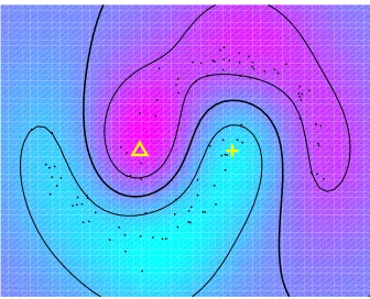
Figure 1: Two moons. There are 2 labeled points (the triangle and the cross) and 100 unlabeled points. The global optimum of S3VM correctly identifies the decision boundary (black line).
points in a data cluster have similar labels (Seeger, 2006; Chapelle and Zien, 2005). Figure 1 illus-trates a low-density decision surface implementing the cluster assumption on a toy two-dimensional data set. This idea was first introduced by Vapnik and Sterin (1977) under the name Transduc-tive SVM, but since it learns an inducTransduc-tive rule defined over the entire input space, we refer to this approach as Semi-Supervised SVM (S3VM).
Since its first implementation by Joachims (1999), a wide spectrum of techniques have been applied to solve the non-convex optimization problem associated with S3VMs, for example, local combinatorial search (Joachims, 1999), gradient descent (Chapelle and Zien, 2005), continuation techniques (Chapelle et al., 2006a), convex-concave procedures (Fung and Mangasarian, 2001; Collobert et al., 2006), semi-definite programming (Bie and Cristianini, 2006; Xu et al., 2004), non-differentiable methods (Astorino and Fuduli, 2007), deterministic annealing (Sindhwani et al., 2006), and branch-and-bound algorithms (Bennett and Demiriz, 1998; Chapelle et al., 2006c).
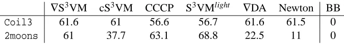
While non-convexity is partly responsible for this diversity of methods, it is also a departure from one of the nicest aspects of SVMs. Table 1 benchmarks the empirical performance of various S3VM implementations against the globally optimal solution obtained by a Branch-and-Bound al-gorithm. These empirical observations strengthen the conjecture that the performance variability of S3VM implementations is closely tied to their susceptibility to sub-optimal local minima. Together with several subtle implementation differences, this makes it challenging to cross-compare different S3VM algorithms.
The aim of this paper is to provide a review of optimization techniques for semi-supervised SVMs and to bring different implementations, and various aspects of their empirical performance, under a common experimental setting.
∇S3VM cS3VM CCCP S3VMlight ∇DA Newton BB
Coil3 61.6 61 56.6 56.7 61.6 61.5 0
2moons 61 37.7 63.1 68.8 22.5 11 0
Table 1: Generalization performance (error rates) of different S3VM algorithms on two (small) data
sets Coil3 and2moons. Branch and Bound (BB) yields the globally optimal solution
which gives perfect separation. BB can only be applied to small data sets due to its high computational costs. See Section 5 for experimental details.
2. Semi-Supervised Support Vector Machines
We consider the problem of binary classification. The training set consists of l labeled examples {(xi,yi)}li=1, yi=±1, and u unlabeled examples{xi}ni=l+1, with n=l+u. In the linear S3VM clas-sification setting, the following minimization problem is solved over both the hyperplane parameters (w,b)and the label vector yu:= [yl+1. . .yn]>,
min
(w,b),yu
I
(w,b,yu) =1 2kwk
2+C
∑
li=1
V(yi,oi) +C? n
∑
i=l+1
V(yi,oi) (1)
where oi=w>xi+b and V is a loss function. The Hinge loss is a popular choice for V ,
V(yi,oi) =max(0,1−yioi)p. (2)
It is common to penalize the Hinge loss either linearly (p=1) or quadratically (p=2). In the rest of the paper, we will consider p=2. Non-linear decision boundaries can be constructed using the kernel trick (Vapnik, 1998).
The first two terms in the objective function
I
in (1) define a standard SVM. The third term incorporates unlabeled data. The loss over labeled and unlabeled examples is weighted by two hyperparameters, C and C?, which reflect confidence in labels and in the cluster assumption respec-tively. In general, C and C?need to be set at different values for optimal generalization performance.The minimization problem (1) is solved under the following class balancing constraint,
1 u
n
∑
i=l+1
max(yi,0) =r or equivalently
1 u
n
∑
i=l+1
yi=2r−1. (3)
This constraint helps in avoiding unbalanced solutions by enforcing that a certain user-specified fraction, r, of the unlabeled data should be assigned to the positive class. It was introduced with the first S3VM implementation (Joachims, 1999). Since the true class ratio is unknown for the unlabeled data, r is estimated from the class ratio on the labeled set, or from prior knowledge about the classification problem.
There are two broad strategies for minimizing
I
:1. Combinatorial Optimization: For a given fixed yu, the optimization over(w,b)is a standard
SVM training.1 Let us define:
J
(yu) =minw,b
I
(w,b,yu). (4)The goal now is to minimize
J
over a set of binary variables. This combinatorial view of the optimization problem is adopted by Joachims (1999), Bie and Cristianini (2006), Xu et al. (2004), Sindhwani et al. (2006), Bennett and Demiriz (1998), and Chapelle et al. (2006c). There is no known algorithm that finds the global optimum efficiently. In Section 3 we review this class of techniques.2. Continuous Optimization: For a fixed (w,b), arg minyV(y,o) =sign(o). Therefore, the
optimal yuis simply given by the signs of oi=w>xi+b. Eliminating yuin this manner gives
a continuous objective function over(w,b):
1 2kwk
2+C
∑
li=1
max(0,1−yioi)2+C? n
∑
i=l+1
max(0,1− |oi|)2. (5)
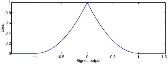
This form of the optimization problem illustrates how S3VMs implement the cluster assump-tion. The first two terms in (5) correspond to a standard SVM. The last term (see Figure 2) drives the decision boundary, that is, the zero output contour, away from unlabeled points. From Figure 2, it is clear that the objective function is non-convex.
−1 −0.5 0 0.5 1 1.5
0 0.2 0.4 0.6 0.8 1
Signed output
Loss
Figure 2: The effective loss max(0,1− |o|)2 is shown above as a function of o= (w>x+b), the real-valued output at an unlabeled point x.
Note that in this form, the balance constraint becomes1u∑ni=l+1sign(w>xi+b) =2r−1 which
is non-linear in(w,b)and not straightforward to enforce. In Section 4 we review this class of methods (Chapelle and Zien, 2005; Chapelle et al., 2006a; Fung and Mangasarian, 2001; Collobert et al., 2006).
3. Combinatorial Optimization
We now discuss combinatorial techniques in which the labels yuof the unlabeled points are explicit
optimization variables. Many of the techniques discussed in this section call a standard (or slightly modified) supervised SVM as a subroutine to perform the minimization over(w,b) for a fixed yu
3.1 Branch-and-Bound (BB) for Global Optimization
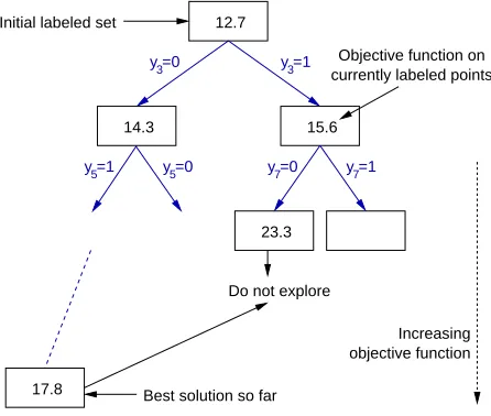
The objective function (4) can be globally optimized using Branch-and-Bound techniques. This was noted in the context of S3VM by Wapnik and Tscherwonenkis (1979) but no details were presented there. In general, global optimization can be computationally very demanding. The technique described in this section is impractical for large data sets. However, with effective heuristics it can produce globally optimal solutions for small-sized problems. This is useful for benchmarking practical S3VM implementations. Indeed, as Table 1 suggests, the exact solution can return excellent generalization performance in situations where other implementations fail completely. Branch-and-Bound was first applied by Bennett and Demiriz (1998) in association with integer programming for solving linear S3VMs. More recently Chapelle et al. (2006c) presented a Branch-and-Bound (BB) algorithm which we outline in this section. The main ideas are illustrated in Figure 3.
objective function Initial labeled set
y =0
y =15
Increasing Do not explore
Best solution so far
3
y =07 7 y =05
3 y =1
y =1
Objective function on currently labeled points 12.7
15.6
17.8
14.3
23.3
Figure 3: Branch-and-Bound Tree
Branch-and-Bound effectively performs an exhaustive search over yu, pruning large parts of
the solution space based on the following simple observation: suppose that a lower bound on minyu∈A
J
(yu), for some subset A of candidate solutions, is greater thanJ
(˜yu) for some ˜yu, thenA can be safely discarded from exhaustive search. BB organizes subsets of solutions into a binary tree (Figure 3) where nodes are associated with a fixed partial labeling of the unlabeled data set and the two children correspond to the labeling of some new unlabeled point. Thus, the root corresponds to the initial set of labeled examples and the leaves correspond to a complete labeling of the data. Any node is then associated with the subset of candidate solutions that appear at the leaves of the subtree rooted at that node (all possible ways of completing the labeling, given the partial labeling at that node). This subset can potentially be pruned from the search by the Branch-and-Bound pro-cedure if a lower bound over corresponding objective values turns out to be worse than an available solution.
set.2 As one goes down the tree, this objective value increases as additional loss terms are added, and eventually equals
J
at the leaves. Note that once a node violates the balance constraint, it can be immediately pruned by resetting its lower bound to∞. Chapelle et al. (2006c) use a labeling-confidence criterion to choose an unlabeled example and a label on which to branch. The tree is explored on the fly by depth-first search. This confidence-based tree exploration is also intuitively linked to Label Propagation methods (Zhu and Ghahramani, 2002) for graph-transduction. On many small data sets (e.g., Table 1 data sets have up to 200 examples) BB is able to return the globally optimal solution in reasonable amount of time. We point the reader to Chapelle et al. (2006c) for pseudocode.3.2 S3VMlight
S3VMlight(Joachims, 1999) refers to the first S3VM algorithm implemented in the popular SVMlight software.3 It is based on local combinatorial search guided by a label switching procedure. The vector yu is initialized as the labeling given by an SVM trained on the labeled set, thresholding
outputs so that u×r unlabeled examples are positive. Subsequent steps in the algorithm comprise of switching labels of two examples in opposite classes, thus always maintaining the balance con-straint. Consider an iteration of the algorithm where yuis the temporary labeling of the unlabeled
data and let(w˜,˜b) =argminw,b
I
(w,b,yu) andJ
(yu) =I
(w˜,˜b,yu). Suppose a pair of unlabeledexamples indexed by(i,j)satisfies the following condition,4
yi=1,yj=−1,V(1,oi) +V(−1,oj)>V(−1,oi) +V(1,oj) (6)
where oi,oj are outputs of (w˜,˜b) on the examples xi,xj. Then after switching labels for this
pair of examples and retraining, the objective function
J
can be easily shown to strictly decrease. S3VMlight alternates between label-switching and retraining. Since the number of possible yu isfinite, the procedure is guaranteed to terminate in a finite number of steps at a local minima of (4), that is, no further improvements are possible by interchanging two labels.
In an outer loop, S3VMlight gradually increases the value of C? from a small value to the final value. Since C? controls the non-convex part of the objective function (4), this annealing loop can be interpreted as implementing a “smoothing” heuristic as a means to protect the algorithm from sub-optimal local minima. The pseudocode is provided in Algorithm 1.
3.3 Deterministic Annealing S3VM
Deterministic annealing (DA) is a global optimization heuristic that has been used to approach hard combinatorial or non-convex problems. In the context of S3VMs (Sindhwani et al., 2006), it consists of relaxing the discrete label variables yuto real-valued variables pu= (pl+1, . . . ,pl+u)where piis
interpreted as the probability that yi=1. The following objective function is now considered:
I
0(w,b,pu) = E[
I
(w,b,yu)] (7)= 1
2kwk
2+C
∑
li=1
V(yi,oi) +C? n
∑
i=l+1
piV(1,oi) + (1−pi)V(−1,oi)
2. Note that in this SVM training, the loss terms associated with (originally) labeled and (currently labeled) unlabeled examples are weighted by C and C?respectively.
Algorithm 1 S3VMlight
Train an SVM with the labeled points. oi←w·xi+b.
Assign yi←1 to the ur largest oi, -1 to the others.
˜
C←10−5C?
while ˜C<C?do repeat
Minimize (1) with{yi}fixed and C?replaced by ˜C.
if∃(i,j)satisfying (6) then Swap the labels yi and yj
end if
until No labels have been swapped
˜
C←min(1.5C,C?) end while
where E denotes expectation under the probabilities pu. Note that at optimality with respect to pu,
pimust concentrate all its mass on yi=sign(w>xi+b)which leads to the smaller of the two losses
V(1,oi)and V(−1,oi). Hence, this relaxation step does not lead to loss of optimality and is simply
a reformulation of the original objective in terms of continuous variables. In DA, an additional entropy term−H(pu)is added to the objective,
I
00(w,b,pu; T) =
I
0(w,b,pu)−T H(pu)where H(pu) =−
∑
ipilog pi+ (1−pi) log (1−pi),
and T ≥0 is usually referred to as ‘temperature’. Instead of (3), the following class balance con-straint is used,
1 u
n
∑
i=l+1 pi=r.
Note that when T =0,
I
00reduces to (7) and the optimal puidentifies the optimal yu. When T =∞,I
00is dominated by the entropy term resulting in the maximum entropy solution (pi=r for all i). T
parameterizes a family of objective functions with increasing degrees of non-convexity (see Figure 4 and further discussion below).
At any T , let(wT,bT,puT) =argmin(w,b),puI
00(w,b,p
u; T). This minimization can be performed
in different ways:
1. Alternating Minimization: We sketch here the procedure proposed by Sindhwani et al. (2006). Keeping pu fixed, the minimization over (w,b) is standard SVM training—each unlabeled
example contributes two loss terms weighted by C?piand C?(1−pi). Keeping(w,b)fixed,
I00 is minimized subject to the balance constraint 1u∑ni=l+1pi=r using standard Lagrangian
techniques. This leads to:
pi=
1
1+e(gi−ν)/T (8)
where gi=C?[V(1,oi)−V(−1,oi)]andν, the Lagrange multiplier associated with the balance
constraint, is obtained by solving the root finding problem that arises by plugging (8) back in the balance constraint. The alternating optimization proceeds until pustabilizes in a
2. Gradient Methods: An alternative possibility5is to substitute the optimal pu(8) as a function
of(w,b) and obtain an objective function over(w,b) for which gradient techniques can be used:
S
(w,b):=minpu
I
00(w,b,p
u; T). (9)
S
(w,b)can be minimized by conjugate gradient descent. The gradient ofS
is easy to com-pute. Indeed, let us denote by p∗u(w,b)the argmin of (9). Then,∂
S
∂wi
=∂
I
00
∂wi
+
n
∑
j=l+1 ∂
I
00∂pj
pu=p∗u(w,b)
| {z }
0
∂p∗j(w)
∂wi
=∂
I
0(w,b,p? u(w))
∂wi .
The partial derivative of
I
00with respect to pjis 0 by the definition of p∗u(w,b). The argumentgoes through even in the presence of the constraint 1u∑pi=r; see Chapelle et al. (2002,
Lemma 2) for a formal proof. In other words, we can compute the gradient of (7) with respect to w and consider pufixed. The same holds for b. This method will be referred to as∇DA in
the rest of the paper.
Figure 4 shows the effective loss terms in
S
associated with an unlabeled example for various values of T . In an outer loop, starting from a high value, T is decreased geometrically by a con-stant factor. The vector pu is then tightened back close to discrete values (its entropy falls belowsome threshold), thus identifying a solution to the original problem. The pseudocode is provided in Algorithm 2.
Table 2 compares the DA and∇DA solutions as T →0 at two different hyperparameter set-tings.6 Because DA does alternate minimization and∇DA does direct minimization, the solutions returned by them can be quite different. Since∇DA is faster than DA, we only report∇DA results in the Section 5.
Algorithm 2 DA/∇DA
Initialize pi=r i=l+1, . . . ,n
Set T =10C?, R=1.5, ε=10−6.
while H(puT)>εdo
Solve(wT,bT,puT) =argmin(w,b),pu
I
00(w,b,p
u; T) subject to: 1u∑in=l+1pi=r
(find local minima starting from previous solution—alternating optimization or gradient meth-ods can be used.)
T =T/R
end while
Return wT,bT
3.4 Convex Relaxation
We follow Bie and Cristianini (2006) in this section, but outline the details for the squared Hinge loss (see also Xu et al., 2004, for a similar derivation). Rewriting (1) as the familiar constrained
−3 −2 −1 0 1 2 3 −2
−1.5 −1 −0.5 0 0.5 1
output
loss
Decreasing T
Figure 4: DA parameterizes a family of loss functions (over unlabeled examples) where the degree of non-convexity is controlled by T . As T →0, the original loss function (Figure 2) is recovered.
DA ∇DA DA ∇DA
g50c 6.5 7 8.3 6.7
Text 13.6 5.7 6.2 6.5
Uspst 22.5 27.2 11 11
Isolet 38.3 39.8 28.6 26.9
Coil20 3 12.3 19.2 18.9
Coil3 49.1 61.6 60.3 60.6
2moons 36.8 22.5 62.1 30
Table 2: Generalization performance (error rates) of the two DA algorithms. DA is the original algorithm (alternate optimization on puand w). ∇DA is a direct gradient optimization on
(w,b), where pushould be considered as a function of(w,b). The first two columns report
results when C?=C and the last columns report results when C?=C/100. See Section 5 for more experimental details.
optimization problem of SVMs:
min
(w,b),yu
1 2kwk
2+C
∑
li=1 ξ2
i +C? n
∑
i=l+1 ξ2
i subject to: yioi≥1−ξi i=1, . . . ,n.
Consider the associated dual problem:
min
{yi}
max α
n
∑
i=1 αi−
1 2
n
∑
i,j=1
αiαjyiyjKi j subject to: n
∑
i=1
αiyi=0, αi≥0
where Ki j=x>i xj+Di jand D is a diagonal matrix given by Dii=2C1, i=1, . . . ,l and Dii=2C1?, i=
Introducing an n×n matrixΓ, the optimization problem can be reformulated as:
min Γ maxα
n
∑
i=1 αi−
1 2
n
∑
i,j=1
αiαjΓi jKi j (10)
under constraints
∑
αiyi=0, αi≥0, Γ=yy>. (11)The objective function (10) is now convex since it is the pointwise supremum of linear functions. However the constraint (11) is not. The idea of the relaxation is to replace the constraintΓ=yy> by the following set of convex constraints:
Γ0,
Γi j =yiyj, 1≤i,j≤l,
Γii=1, l+1≤i≤n.
Though the original method of Bie and Cristianini (2006) does not incorporate the class bal-ancing constraint (3), one can additionally enforce it as u12∑
n
i,j=l+1Γi j = (2r−1)2. Such a soft
constraint is also used in the continuous S3VM optimization methods of Section 4.
The convex problem above can be solved through Semi-Definite Programming. The labels of the unlabeled points are estimated fromΓ(through one of its columns or its largest eigenvector).
This method is very expensive and scales as O((l+u2)2(l+u)2.5). It is possible to try to optimize a low rank version ofΓ, but the training remains slow even in that case. We therefore do not conduct empirical studies with this method.
4. Continuous Optimization
In this section we consider methods which do not include yu, the labels of unlabeled examples, as
optimization variables, but instead solve suitably modified versions of (5) by continuous optimiza-tion techniques. We begin by discussing two issues that are common to these methods.
Balancing Constraint The balancing constraint (3) is relatively easy to enforce for all algorithms presented in Section 3. It is more difficult for algorithms covered in this section. The proposed workaround, first introduced by Chapelle and Zien (2005), is to instead enforce a linear constraint:
1 u
n
∑
i=l+1
w>xi+b=2˜r−1, (12)
where ˜r=r. The above constraint may be viewed as a “relaxation” of (3). For a given ˜r, an easy way of enforcing (12) is to translate all the points such that the mean of the unlabeled points is the origin, that is,∑ni=l+1xi=0. Then, by fixing b=2˜r−1, we have an unconstrained optimization problem
on w. We will assume that the xi are translated and b is fixed in this manner; so the discussion will
focus on unconstrained optimization procedures for the rest of this section. In addition to being easy to implement, this linear constraint may also add some robustness against uncertainty about the true unknown class ratio in the unlabeled set (see also Chen et al., 2003, for related discussion).
However, since (12) relaxes (3),7the solutions found by algorithms in this section cannot strictly be compared with those in Section 3. In order to admit comparisons (this is particularly important for the empirical study in Section 5), we vary ˜r in an outer loop and do a dichotomic search on this value such that (3) is satisfied.
Primal Optimization For linear classification, the variables in w can be directly optimized. Non-linear decision boundaries require the use of the “kernel trick” (Boser et al., 1992) using a kernel function k(x,x0). While most of the methods of Section 3 can use a standard SVM solver as a sub-routine, the methods of this section need to solve (5) with a non-convex loss function over unlabeled examples. Therefore, they cannot directly use off-the-shelf dual-based SVM software. We use one of the following primal methods to implement the techniques in this section.
Method 1 We find zi such that zi·zj =k(xi,xj). If B is a matrix having columns zi, this can
be written in matrix form as B>B=K. The Cholesky factor of K provides one such B. This decomposition was used for∇S3VM (Chapelle and Zien, 2005). Another possibility is to perform the eigendecomposition of K as K=UΛU>and set B=Λ1/2U>. This latter case corresponds to the
kernel PCA map introduced by Sch ¨olkopf and Smola (2002, Section 14.2). Once the zi are found,
we can simply replace xiin (5) by ziand solve a linear classification problem. For more details, see
Chapelle et al. (2006a).
Method 2 We set w=∑ni=1βiφ(xi)whereφdenotes a higher dimensional feature map associated
with the nonlinear kernel. By the Representer theorem (Sch ¨olkopf and Smola, 2002), we indeed know that the optimal solution has this form. Substituting this form in (5) and using the kernel function yields an optimization problem withβas the variables.
Note that the centering mentioned above to implement (12) corresponds to using the modified kernel Sch¨olkopf and Smola (2002, page 431) defined by:
k(x,x0):=k(x,x0)−1 u
n
∑
i=l+1
k(x,xi)−
1 u
n
∑
i=l+1
k(x0,xi) +
1 u2
n
∑
i,j=l+1
k(xi,xj). (13)
All the shifted kernel elements can be computed in O(n2)operations.
Finally, note that these methods are very general and can also be applied to algorithms of Sec-tion 3.
4.1 Concave Convex Procedure (CCCP)
The CCCP method (Yuille and Rangarajan, 2003) has been applied to S3VMs by Fung and Man-gasarian (2001), Collobert et al. (2006), and Wang et al. (2007). The description given here is close to that in Collobert et al. (2006).
CCCP essentially decomposes a non-convex function f into a convex component fvexand a
con-cave component fcave. At each iteration, the concave part is replaced by a linear function (namely,
the tangential approximation at the current point) and the sum of this linear function and the convex part is minimized to get the next iterate. The pseudocode is shown in Algorithm 3.
Algorithm 3 CCCP for minimizing f =fvex+fcave
Require: Starting point x0
t←0
while∇f(xt)6=0 do
xt+1←arg minxfvex(x) +∇fcave(xt)·x
t←t+1
In the case of S3VM, the first two terms in (5) are convex. Splitting the last non-convex term corresponding to the unlabeled part as the sum of a convex and a concave function, we have:
max(0,1− |t|)2=max(0,1− |t|)2+2|t|
| {z }
convex
−2|t|
| {z }
concave
.
If an unlabeled point is currently classified positive, then at the next iteration, the effective (convex) loss on this point will be
˜L(t) =
0 if t≥1,
(1−t)2 if|t|<1, −4t if t≤ −1.
A corresponding ˜L can be defined for the case of an unlabeled point being classified negative. The CCCP algorithm specialized to S3VMs is given in Algorithm 4. For optimization variables we employ method 1 given at the beginning of this section.
Algorithm 4 CCCP for S3VMs
Starting point: Use the w obtained from the supervised SVM solution.
repeat
yi←sign(w·xi+b), l+1≤i≤n.
(w,b) =arg min12kwk2+C∑l
i=1max(0,1−yi(w·xi+b))2+C?∑ni=l+1˜L(yi(w·xi+b)).
until convergence of yi,l+1≤i≤n.
The CCCP method given in Collobert et al. (2006) does not use annealing, that is, increasing C? slowly in steps as in S3VMlight to help reduce local minima problems. We have however found performance improvements with annealing (see Table 12).
4.2 ∇S3VM
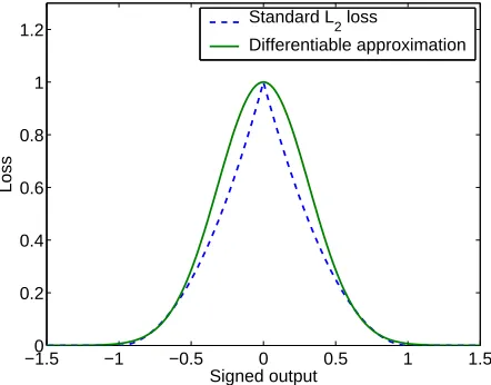
This method is proposed by Chapelle and Zien (2005) to minimize directly the objective function (5) by gradient descent. For optimization variables, method 1 given at the beginning of this section is used. Since the function t7→max(0,1− |t|)2is not differentiable, it is replaced by t7→exp(−st2), with s=5 (see Figure 5), to get the following smooth optimization problem:8
min
w,b
1 2kwk
2+C
∑
li=1
max(0,1−yi(w·xi+b))2+C? n
∑
i=l+1
exp(−s(w·xi+b)2). (14)
As for S3VMlight, ∇S3VM performs annealing in an outer loop on C?. In the experiments we followed the same annealing schedule as in Chapelle and Zien (2005): C?is increased in 10 steps to its final value. More precisely, at the ith step, C?is set to 2i−10C?f inal.
4.3 Continuation S3VM (cS3VM)
Closely related to∇S3VM, Chapelle et al. (2006a) proposes a continuation method for minimizing (14). Gradient descent is performed on the same objective function (with the same loss for the
−1.50 −1 −0.5 0 0.5 1 1.5 0.2
0.4 0.6 0.8 1 1.2
Loss
Signed output Standard L
2 loss
Differentiable approximation
Figure 5: The loss function on the unlabeled points t7→max(0,1− |t|)2is replaced by a differen-tiable approximation t7→exp(−5t2).
unlabeled points as shown in Figure 5), but the method used for annealing is different. Instead of slowly increasing C?, it is kept fixed, and a continuation technique is used to transform the objective function.
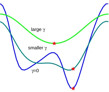
This kind of method belongs to the field of global optimization techniques (Wu, 1996). The idea is similar to deterministic annealing (see Figure 6). A smoothed version of the objective function is first minimized. With enough smoothing the global minimum can hopefully be easily found. Then the smoothing is decreased in steps and the minimum is tracked—the solution found in one step serves as the starting point for the next step. The method is continued until there is no smoothing and so we get back to the solution of (14). Algorithm 5 gives an instantiation of the method in which smoothing is achieved by convolution with a Gaussian, but other smoothing functions can also be used.
Algorithm 5 Continuation method for solving minxf(x)
Require: Function f :Rd7→R, initial point x0∈Rd
Require: Sequenceγ0>γ1> . . .γp−1>γp=0.
Let fγ(x) = (πγ)−d/2R
f(x−t)exp(−ktk2/γ)dt.
for i=0 to p do
Starting from xi, find local minimizer xi+1of fγi.
end for
large γ
γ=0 smaller γ
Figure 6: Illustration of the continuation method: the original objective function in blue has two local minima. By smoothing it, we find one global minimum (the red star on the green curve). By reducing the smoothing, the minimum moves toward the global minimum of the original function.
4.4 Newton S3VM
One difficulty with the methods described in sections 4.2 and 4.3 is that their complexity scales as O(n3)because they employ an unlabeled loss function that does not have a linear part, for example, see (14). Compared to a method like S3VMlight(see Section 3.2), which typically scales as O(n3sv+
n2), this can make a large difference in efficiency when nsv(the number of support vectors) is small.
In this subsection we propose a new loss function for unlabeled points and an associated Newton method (along the lines of Chapelle, 2007) which brings down the O(n3)complexity of the∇S3VM method.
To make efficiency gains we employ method 2 described at the beginning of this section (note that method 1 requires an O(n3) preprocessing step) and perform the minimization onβ, where
w=∑n
i=1βiφ(xi). Note that theβi are expansion coefficients and not the Lagrange multipliersαi
in standard SVMs. Let us consider general loss functions, `L for the labeled points, `U for the
unlabeled points, replace w byβas the variables in (5), and get the following optimization problem,
min β
1 2β
>
Kβ+C
l
∑
i=1
`L(yi(Ki>β+b)) +C? n
∑
i=l+1
`U(Ki>β+b), (15)
where K is the kernel matrix with Ki j =k(xi,xj)and Ki is the ithcolumn of K.9
As we will see in detail below, computational time is dictated by nsv, the number of points that
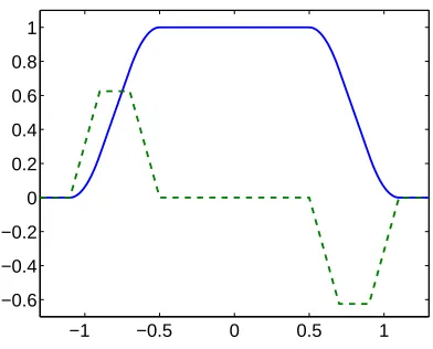
lie in the domain of the loss function where curvature is non-zero. With this motivation we choose the differentiable loss function plotted in Figure 7 having several linear and flat parts which are smoothly connected by small quadratic components.10
9. Note that, the kernel elements used here correspond to the modified kernel elements in (13).
−1 −0.5 0 0.5 1 −0.6
−0.4 −0.2 0 0.2 0.4 0.6 0.8 1
Figure 7: The piecewise quadratic loss function`U and its derivative (divided by 4; dashed line).
Consider the solution of (15) with this choice of loss function. The gradient of (15) is
Kg with gi=
β
i+C`0L(yi(Ki>β+b))yi 1≤i≤l
βi+C?`0U(Ki>β+b) l+1≤i≤n
. (16)
Using a gradient based method like nonlinear conjugate gradient would sill be costly because each evaluation of the gradient requires O(n2)effort. To improve the complexity when nsvis small, one
can use Newton’s method instead. Let us now go into these details. The Hessian of (15) is
K+KDK, with D diagonal, Dii=
C`00L(yi(Ki>β+b)) 1≤i≤l
C?`U00(Ki>β+b) l+1≤i≤n . (17)
The corresponding Newton update isβ←β−(K+KDK)−1Kg. The advantage of Newton opti-mization on this problem is that the step can be computed in O(n3sv+n
2)time11as we will see below (see also Chapelle, 2007, for a similar derivation). The number of Newton steps required is usually a small finite constant.
A problem in performing a Newton optimization with a non-convex optimization function is that the step might not be a descent direction because the Hessian is not necessarily positive definite. To avoid this problem, we use the Levenberg-Marquardt algorithm (Fletcher, 1987, Algorithm 5.2.7). Roughly speaking, this algorithm is the same as Newton minimization, but a large enough ridge is added to the Hessian such that it becomes positive definite. For computational reasons, instead of adding a ridge to the Hessian, we will add a constant times K.
The goal is to choose aλ≥1 such thatλK+KDK is positive definite and solve(λK+KDK)−1Kg efficiently. For this purpose, we reorder the points such that Dii6=0, i≤nsvand Dii=0, i>nsv.
Let A be the Cholesky decomposition of K:12 A is the upper triangular matrix satisfying A>A=K. We suppose that K (and thus A) is invertible. Let us write
λK+KDK=A>(λIn+ADA>)A.
11. Consistent with the way we defined earlier, note here that nsv is the number of “support vectors” where a support vector is defined as a point xisuch that Dii6=0.
The structure of K and D implies that
λK+KDK0⇔B :=λInsv+AsvDsvA > sv0,
where Asv is the Cholesky decomposition of Ksv and Ksv is the matrix formed using the first nsv
rows and columns of K. After some block matrix algebra, we can also get the step as
−(λK+KDK)−1Kg=
A−sv1B −1A
sv(gsv−
1
λDsvKsv,nsvgnsv)
1 λgnsv
, (18)
wherensvrefers to the indices of the ”non support vectors”, that is,{i, Dii=0}. Computing this
direction takes O(n3sv+n
2)operations. The checking of the positive definiteness of B can be done by doing Cholesky decomposition of Ksv. This decomposition can then be reused to solve the linear
system involving B. Full details, following the ideas in Fletcher (1987, Algorithm 5.2.7), are given in Algorithm 6.
Algorithm 6 Levenberg-Marquardt method
β←0. λ←1.
repeat
Compute g and D using (16) and (17)
sv← {i, Dii6=0}andnsv← {i,Dii=0}.
Asv←Cholesky decomposition of Ksv.
Do the Cholesky decomposition ofλInsv+AsvDsvA >
sv. If it fails,λ←4λand try again.
Compute the step s as given by (18). ρ← 1 Ω(β+s)−Ω(β)
2s>(K+KDK)s+s>Kg
. % If the obj funΩwere quadratic,ρwould be 1. Ifρ>0,β←β+s.
Ifρ<0.25,λ←4λ. Ifρ>0.75,λ←min(1,λ2).
until Norm(g)≤ε
As discussed above, the flat part in the loss (cf. Figure 7) provides computational value by reducing nsv. But we feel it may also possibly help in leading to better local minimum. Take
for instance a Gaussian kernel and consider an unlabeled point far from the labeled points. At the beginning of the optimization, the output on that point will be 0.13 This unlabeled point does not contribute to pushing the decision boundary one way or the other. This seems like a satisfactory behavior: it is better to wait to have more information before taking a decision on an unlabeled point for which we are unsure. In Table 3 we compare the performance of the flat loss in Figure 7 and the original quadratic loss used in (5). The flat loss yields a huge gain in performance on2moons. On the other data sets the two losses perform somewhat similarly. From a computational point of view, the flat part in the loss can sometimes reduce the training time by a factor 10 as shown in Table 3.
5. Experiments
This section is organized around a set of empirical issues:
Error rate Training time Flat Quadratic Flat Quadratic
g50c 6.1 5.3 15 39
Text 5.4 7.7 2180 2165
Uspst 18.6 15.9 233 2152
Isolet 32.2 27.1 168 1253
Coil20 24.1 24.7 152 1244
Coil3 61.5 58.4 6 8
2moons 11 66.4 1.7 1.2
Table 3: Comparison of the Newton-S3VM method with two different losses: the one with a flat part in the middle (see Figure 7) and the standard quadratic loss (Figure 2). Left: error rates on the unlabeled set; right: average training time in seconds for one split and one binary classifier training (with annealing and dichotomic search on the threshold as explained in the experimental section). The implementations have not been optimized, so the training times only constitute an estimate of the relative speeds.
1. While S3VMs have been very successful for text classification (Joachims, 1999), there are many data sets where they do not return state-of-the-art empirical performance (Chapelle and Zien, 2005). This performance variability is conjectured to be due to local minima problems. In Section 5.3, we discuss the suitability of the S3VM objective function for semi-supervised learning. In particular, we benchmark current S3VM implementations against the exact, glob-ally optimal solution and we discuss whether one can expect significant improvements in generalization performance by better approaching the global solution.
2. Several factors influence the performance and behavior of S3VM algorithms. In Section 5.4 we study their quality of optimization, generalization performance, sensitivity to hyperpa-rameters, effect of annealing and the robustness to uncertainty in class ratio estimates.
3. S3VMs were originally motivated by Transductive learning, the problem of estimating labels of unlabeled examples without necessarily producing a decision function over the entire input space. However, S3VMs are also semi-supervised learners as they are able to handle unseen test instances. In Section 5.5, we run S3VM algorithms in an inductive mode and analyze performance differences between unlabeled and test examples.
4. There is empirical evidence that S3VMs exhibit poor performances on “manifold” type data (where graph-based methods typically excel) or when the data has many distinct sub-clusters (Chapelle and Zien, 2005). We explore the issue of data geometry and S3VM performance in Section 5.6.
semi-supervised tasks. Our goal, therefore, is not so much to establish a ranking of algorithms reviewed in this paper, but rather to observe their behavior under a neutral experimental protocol.
We next describe the data sets used in our experiments. Note that our choice of data sets is biased towards multi-class manifold-like problems which are particularly challenging for S3VMs. Because of this choice, the experimental results do not show the typically large improvements one might expect over standard SVMs. We caution the reader not to draw the conclusion that S3VM is a weak algorithm in general, but that it often does not return state-of-the-art performance on problems of this nature.
5.1 Data Sets
Most data sets come from Chapelle and Zien (2005). They are summarized in Table 4.
data set classes dims points labeled
g50c 2 50 550 50
Text 2 7511 1946 50
Uspst 10 256 2007 50
Isolet 9 617 1620 50
Coil20 20 1024 1440 40
Coil3 3 1024 216 6
2moons 2 102 200 2
Table 4: Basic properties of benchmark data sets.
The artificial data setg50cis inspired by Bengio and Grandvalet (2004): examples are generated from two standard normal multi-variate Gaussians, the labels correspond to the Gaussians, and the means are located in 50-dimensional space such that the Bayes error is 5%. The real world data sets consist of two-class and multi-class problems. The Text data set is defined using the classesmacandmswindowsof theNewsgroup20data set preprocessed as in Szummer and Jaakkola (2001). The Uspst set contains the test data part of the well-known USPS data on handwritten digit recognition. TheIsoletis a subset of the ISOLET spoken letter database (Cole et al., 1990) containing the speaker sets 1, 2 and 3 and 9 confusing letters {B,C,D,E,G,P,T,V,Z}. In Coil20
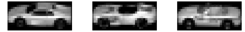
(respectivelyCoil3), the data are gray-scale images of 20 (respectively 3) different objects taken from different angles, in steps of 5 degrees (Nene et al., 1996). TheCoil3data set has been used first by Chapelle et al. (2006c) and is particularly difficult since the 3 classes are 3 cars which look alike (see Figure 8).
Finally, 2moons has been used extensively in the semi-supervised learning literature (see for instance Zhu and Ghahramani, 2002, and Figure 1). For this data set, the labeled points are fixed and new unlabeled points are randomly generated for each repetition of the experiment.
5.2 Experimental Setup
To minimize the influence of external factors, unless stated otherwise, the experiments were run in the following normalized way:
Hyperparameters The Gaussian kernel k(x,y) =exp(−kx−yk2/2σ2)was used. For simplicity the constant C? in (1) was set to C.14 The same hyperparameters C andσ have been used for all the methods. They are found with cross-validation by training an inductive SVM on the entire data set (the unlabeled points being assigned their real label). These values are reported in Table 5. Even though it seems fair to compare the algorithms with the same hyperparameters, there is a possibility that some regime of hyperparameter settings is more suitable for a particular algorithm than for another. We discuss this issue in section 5.4.3.
Multi-class Data sets with more than two classes are learned with a one-versus-the-rest approach.
The reported objective value is the mean of the objective values of the different classifiers. We also conducted experiments on pair-wise binary classification problems (cf. Section 5.6.1) constructed from the multi-class data sets.
Objective value Even though the objective function that we want to minimize is (5), some
algo-rithms like∇S3VM use another (differentiable) objective function. In order to compare the objective values of the different algorithms, we do the following: after training, we predict the labels of the unlabeled points and train a standard SVM on this augmented labeled set (with p=2 in (2) and C, C? weightings on originally labeled and unlabeled terms respectively). The objective value reported is the one of this SVM.
Balancing constraint For the sake of simplicity, we set r in the balancing constraint (3) to the true
ratio of the positive points in the unlabeled set. This constraint is relatively easy to enforce for all algorithms presented in Section 3. It is more difficult for algorithms in Section 4 and, for them we used the dichotomic search described at the beginning of Section 4.
For a given data set, we randomly split the data into a labeled set and an unlabeled set. We refer to the error rate on the unlabeled set as the unlabeled error to differentiate it from the test error which would be computed on an unseen test set. Results are averaged over 10 random splits. The difference between unlabeled and test performance is discussed in Section 5.5.
5.3 Suitability of the S3VM Objective Function
Table 1 shows unlabeled error rates for common S3VM implementations on two small data sets
Coil3and2moons. On these data sets, we are able to also run Branch-and-Bound and get the true
σ C
g50c 38 19
Text 3.5 31
Uspst 7.4 38
Isolet 15 43
Coil20 2900 37
Coil3 3000 100
2moons 0.5 10
Table 5: Values of the hyperparameters used in the experiments.
though the performance of practical S3VM may not consistently reflect this due to local minima problems.
Table 6 records the rank correlation between unlabeled error and objective function. The rank correlation has been computed in the following way. For each split, we take 10 different solutions and compute the associated unlabeled error and objective value. Ideally, we would like to sam-ple these solutions at random around local minima. But since it is not obvious how to do such a sampling, we simply took the solution given by the different S3VM algorithms as well as 4 “inter-mediate” solutions obtained as follows. A standard SVM is trained on the original labeled set and a fraction of the unlabeled set (with their true labels). The fraction was either 0, 10, 20 or 30%. The labels of the remaining unlabeled points are assigned through a thresholding of the real value outputs of the SVM. This threshold is such that the balancing constraint (3) is satisfied. Finally, an SVM is retrained using the entire training set. By doing so, we “sample” solutions varying from an inductive SVM trained on only the labeled set to the optimal solution. Table 6 provides evidence that the unlabeled error is correlated with the objective values.
Coefficient
g50c 0.2
Text 0.67
Uspst 0.24
Isolet 0.23
Coil20 0.4
Coil3 0.17
2moons 0.45
Table 6: Kendall’s rank correlation (Abdi, 2006) between the unlabeled error and the objective function averaged over the 10 splits (see text for details).
5.4 Behavior of S3VM Algorithms
5.4.1 QUALITY OFMINIMIZATION
In Table 7 we compare different algorithms in terms of minimization of the objective function. ∇S3VM and cS3VM appear clearly to be the methods achieving the lowest objective values. How-ever, as we will see in the next section, this does not necessarily translate into lower unlabeled errors.
∇S3VM cS3VM CCCP S3VMlight ∇DA Newton
1.7 1.9 4.5 4.9 4.3 3.7
Table 7: For each data set and each split, the algorithms were ranked according to the objective function value they attained. This table shows the average ranks. These ranks are only about objective function values; error rates are discussed below.
5.4.2 QUALITY OFGENERALIZATION
Table 8 reports the unlabeled errors of the different algorithms on our benchmark data sets. A first observation is that most algorithms perform quite well ong50candText. However, the unlabeled errors on the other data sets,Uspst,Isolet,Coil20,Coil3,2moons(see also Table 1) are poor and sometimes even worse than a standard SVM. As pointed out earlier, these data sets are particularly challenging for S3VMs. Moreover, the honors are divided and no algorithm clearly outperforms the others. We therefore cannot give a recommendation on which one to use.
∇S3VM cS3VM CCCP S3VMlight ∇DA Newton SVM SVM-5cv
g50c 6.7 6.4 6.3 6.2 7 6.1 8.2 4.9
Text 5.1 5.3 8.3 8.1 5.7 5.4 14.8 2.8
Uspst 15.6 36.2 16.4 15.5 27.2 18.6 20.7 3.9
Isolet 25.8 59.8 26.7 30 39.8 32.2 32.7 6.4
Coil20 25.6 30.7 26.6 25.3 12.3 24.1 24.1 0
Table 8: Unlabeled errors of the different S3VMs implementations. The next to the last column is an SVM trained only on the labeled data, while the last column reports 5 fold cross-validation results of an SVM trained on the whole data set using the labels of the unlabeled points. The values in these two columns can be taken as upper and lower bounds on the best achievable error rates. See Table 1 for results onCoil3and2moons.
binary problems were considered for the cS3VM algorithm, while results in Table 8 for multiclass data sets are obtained under a one-versus-the-rest setup.
5.4.3 SENSITIVITY TOHYPERPARAMETERS
As mentioned before, it is possible that different algorithms excel in different hyperparameter regimes. This is more likely to happen due to better local minima at different hyperparameters as opposed to a better global solution (in terms of error rates).
Due to computational constraints, instead of setting the three hyperparameters (C,C? and the Gaussian kernel width,σ) by cross-validation for each of the methods, we explored the influence of these hyperparameters on one split of the data. More specifically, Table 9 shows the relative improvement (in %) that one can gain by selecting other hyperparameters. These numbers may be seen as a measure of the robustness of a method. Note that these results have to be interpreted carefully because they are only on one split: for instance, it is possible that“by chance” the method did not get stuck in a bad local minimum for one of the hyperparameter settings, leading to a larger number in Table 9.
∇S3VM cS3VM CCCP S3VMlight ∇DA Newton
g50c 31.2 31.2 27.8 13.3 35 7.7
Text 22 7.1 29.2 19.9 34.4 1.1
Uspst 12 70.2 19.2 0 41 15.6
Isolet 7.6 57.6 8 0 4.9 2.6
Coil20 46.4 42.7 27.9 5.8 5.7 16.9
Coil3 32.6 39.2 15.3 20.2 5.8 24.6
2moons 45.6 50 54.1 13.5 23.5 0
Mean 28.2 42.6 25.9 10.4 21.5 9.8
Table 9: On the 1st split of each data set, 27 set of hyperparameters(σ0,C0,C?0) have been tested fromσ0 ∈ {1
2σ,σ,2σ},C
0∈ {1
10C,C,10C},C
?0 ∈ { 1 100C
0, 1 10C
0,C0}. The table shows the
relative improvement (in %) by taking the best hyperparameters over default ones.
By measuring the variation of the unlabeled errors with respect to the choice of the hyperpa-rameters, Table 10 records an indication of the sensitivity of the method with respect to that choice. From this point of view S3VMlight appears to be the most stable algorithm.
∇S3VM cS3VM CCCP S3VMlight ∇DA Newton
6.8 8.5 6.5 2.7 8.4 8.7
Finally, from the experiments in Table 9, we observed that in some cases a smaller value of C? is helpful. We have thus rerun the algorithms on all the splits with C?divided by 100: see Table 11. The overall performance does not necessarily improve, but the very poor results become better (see for instanceUspst,Isolet,Coil20for cS3VM).
∇S3VM cS3VM CCCP S3VMlight ∇DA Newton
g50c 8.3 8.3 8.5 8.4 6.7 7.5
Text 5.7 5.8 8.5 8.1 6.5 14.5
Uspst 14.1 15.6 14.9 14.5 11 19.2
Isolet 27.8 28.5 25.3 29.1 26.9 32.1
Coil20 23.9 23.6 23.6 21.8 18.9 24.6
Coil3 60.8 55.0 56.3 59.2 60.6 60.5
2moons 65.0 49.8 66.3 68.7 30 33.5
Table 11: Same as Table 8, but with C?divided by 100.
5.4.4 EFFECT OFANNEALINGSCHEDULE
All the algorithms described in this paper use some sort of annealing (e.g., gradually decreasing T in DA or increasing C? in S3VMlight in an outer loop) where the role of the unlabeled points is progressively increased. The three ingredients to fix are:
1. The starting point which is usually chosen in such a way that the unlabeled points have very little influence and the problem is thus almost convex.
2. The stopping criterion which should be such that the annealed objective function and the original objective function are very close.
3. The number of steps. Ideally, one would like to have as many steps as possible, but for computational reasons the number of steps is limited.
In the experimental results presented in Figure 9, we only varied the number of steps. The start-ing and final values are as indicated in the description of the algorithms. The original CCCP paper did not have annealing and we used the same scheme as for∇S3VM: C?is increased exponentially from 10−3C to C. For DA and∇DA, the final temperature is fixed at a small constant and the de-crease rate R is such that we have the desired number of steps. For all algorithms, one step means that there is no annealing.
One has to be cautious when drawing conclusion from this plot. Indeed, the results are only for one data set, one split and fixed hyperparameters. The goal is to get an idea of whether the annealing for a given method is useful; and if so, how many steps should be taken. From this plot, it seems that:
• All methods, except Newton, seem to benefit from annealing. However, on some other data sets, annealing improved the performances of Newton’s method (results not shown).
1 2 4 8 16 32 0
0.1 0.2 0.3 0.4
Number of steps
Test error
∇−S3
VM
cS3VM CCCP SVMlight DA Newton ∇DA
Figure 9: Influence of the number of annealing steps on the first split ofText.
No annealing Annealing
g50c 7.9 6.3
Text 14.7 8.3
Uspst 21.3 16.4
Isolet 32.4 26.7
Coil20 26.1 26.6
Coil3 49.3 56.6
2moons 67.1 63.1
Table 12: Performance of CCCP with and without annealing. The annealing schedule is the same as the one used for∇S3VM and Newton: C?is increased in 10 steps from its final value divided by 1000.
• DA seems the method which relies the most on a relatively slow annealing schedule, while ∇DA can have a faster annealing schedule.
• CCCP was originally proposed without annealing, but it seems that its performance can be improved by annealing. To confirm this fact, Table 12 compares the results of CCCP with and without annealing on the 10 splits of all the data sets.
The results provided in Table 8 are with annealing for all methods.
5.4.5 ROBUSTNESS TOCLASSRATIOESTIMATE
Of course, in practice the true number of positive points is unknown. One can estimate it from the labeled points as:
r=1
2 1
l
l
∑
i=1 yi+1
!
.
Table 13 presents the generalization performances in this more realistic context where class ratios are estimated as above and original soft balance constraint is used where applicable (recall the discussion in Section 4).
∇S3VM cS3VM CCCP S3VMlight ∇DA Newton SVM
g50c 7.2 6.6 6.7 7.5 8.4 5.8 9.1
Text 6.8 5 12.8 9.2 8.1 6.1 23.1
Uspst 24.1 41.5 24.3 24.4 29.8 25 24.2
Isolet 48.4 58.3 43.8 36 46 45.5 38.4
Coil20 35.4 51.5 34.5 25.3 12.3 25.4 26.2
Coil3 64.4 59.7 59.4 56.7 61.7 62.9 51.8
2moons 62.2 33.7 55.6 68.8 22.5 8.9 44.4
Table 13: Constant r estimated from the labeled set. For methods of Section 4, the original con-straint (12) is used; there is no dichotomic search (see beginning of Section 4).
5.5 Transductive Versus Semi-supervised Learning
S3VMs were introduced as Transductive SVMs, originally designed for the task of directly estimat-ing labels of unlabeled points. However S3VMs provide a decision boundary in the entire input space, and so they can provide labels of unseen test points as well. For this reason, we believe that S3VMs are inductive semi-supervised methods and not strictly transductive. A discussion on the differences between semi-supervised learning and transduction can be found in Chapelle et al. (2006b, Chapter 25).15
We expect S3VMs to perform equally well on the unlabeled set and on an unseen test set. To test this hypothesis, we took out 25% of the unlabeled set that we used as a unseen test set. We performed 420 experiments (6 algorithms, 7 data sets and 10 splits). Based on these 420 pairs of error rates, we did not observe a significant difference at the 5% confidence level. Also, for each of the 7 data sets (resp 6 algorithms), there was no statistical significant differences in the 60 (resp 70) pairs of error rates.
Similar experiments were performed by Collobert et al. (2006, Section 6.2). Based on 10 splits, the error rate was found to be better on the unlabeled set than on the test set. The authors made the hypothesis that when the test and training data are not identically distributed, transduction can be helpful. Indeed, because of small sample effect, the unlabeled and test set could appear as not coming from the same distribution (this is even more likely in high dimension).
We considered the g50cdata set and biased the split between unlabeled and test set such that there is an angle between the principal directions of the two sets. Figure 10 shows a correlation
0.4 0.5 0.6 0.7 0.8 0.9 1 1.1 −0.2
−0.15 −0.1 −0.05 0 0.05
Angle
Error difference
Figure 10: The test set of g50c has been chosen with a bias such that there is an angle between the principal directions of the unlabeled and test sets. The figure shows the difference in error rates (negative means better error rate on the unlabeled set) as a function of the angle for different random (biased) splits.
between the difference in error rates and this angle: the error on the test set deteriorates as the angle increases. This confirms the hypothesis stated above.
5.6 Role of Data Geometry
There is empirical evidence that S3VMs exhibit poor performances on “manifold” type data or when the data has many distinct sub-clusters (Chapelle and Zien, 2005). We now explore this issue and propose an hybrid method combining the S3VM and LapSVM (Sindhwani et al., 2005).
5.6.1 EFFECT OFMULTIPLECLUSTERS
In Chapelle et al. (2006a), cS3VM exhibited poor performance in multiclass problems with one-versus-the-rest training, but worked well on pairwise binary problems that were constructed (using all the labels) from the same multiclass data sets. Note that in practice it is not possible to do semi-supervised one-vs-one multiclass training because the labels of the unlabeled points are truly unknown.
We compared different algorithms on pairwise binary classification tasks for all the multiclass problems. Results are shown in the first 4 rows of Table 14. Except onCoil3, most S3VM algo-rithms show improved performances. There are two candidate explanations for this behavior:
∇S3VM cS3VM CCCP S3VMlight ∇DA Newton SVM SVM-5cv
Uspst 1.9 2 2.8 2.9 4 1.9 5.3 0.9
Isolet 4.8 11.8 5.5 5.7 5 6.3 7.3 1.2
Coil20 2.8 3.9 2.9 3.1 2.7 2.4 3.3 0
Coil3 45.8 48.7 40.3 41.3 44.5 47.2 36.7 0
Uspst2 15.6 25.7 16.6 16.1 20 16 17.7 3
Table 14: Experiments in a pairwise binary setting.Uspst2is the same set asUspstbut where the task is to classify digits 0 to 4 versus 5 to 9.
2. In a one-versus-the-rest approach, the negative class is the concatenation of several classes and is thus made up of several clusters. This might accentuate the local minimum problem of S3VMs.
To test these hypothesis, we created a binary version ofUspstby classifying digits 0 to 4 versus 5 to 9: this data set (Uspst2in Table 14) is balanced but each class is made of several clusters. The fact that the S3VMs algorithms were not able to perform significantly better than the SVM baseline tends to accredit the second hypothesis: S3VM results deteriorate when there are several clusters per class.
5.6.2 HYBRIDS3VM-GRAPHMETHODS
Recall that the results in Table 8 boost the empirical evidence that S3VMs do not return state-of-the-art performance on “manifold”-like data sets. On these data sets the cluster assumption is presumably satisfied under an intrinsic “geodesic” distance rather than the original euclidean distance between data points. It is reasonable, therefore, to attempt to combine S3VMs with choices of kernels that conform to the particular geometry of the data.
LapSVM (Sindhwani et al., 2005) is a popular semi-supervised algorithm in which a kernel function is constructed from the Laplacian of an adjacency graph that models the data geometry; this kernel is then used with a standard SVM. This procedure was shown to be very effective on data sets with a manifold structure. In Table 15 we report results with a hybrid S3VM-graph method: the kernel is constructed as in LapSVM,16but then it is plugged into S3VMlight. Such a hybrid was first described in Chapelle et al. (2006a) where cS3VM was combined with LapSVM.
The results of this hybrid method is very satisfactory, often outperforming both LapSVM and S3VMlight.
Such a method complements the strengths of both S3VM and Graph-based approaches: the S3VM adds robustness to the construction of the graph, while the graph enforces the right cluster structure to alleviate local minima problems in S3VMs. We believe that this kind of technique is probably one of the most robust and powerful way for a semi-supervised learning problem.
Exact r (Table 8 setting) Estimated r (Table 13 setting) LapSVM S3VMlight LapSVM-S3VMlight S3VMlight LapSVM-S3VMlight
g50c 6.4 6.2 4.6 7.5 6.1
Text 11 8.1 8.3 9.2 9.0
Uspst 11.4 15.5 8.8 24.4 19.6
Isolet 41.2 30.0 46.5 36.0 49.0
Coil20 11.9 25.3 12.5 25.3 12.5
Coil3 20.6 56.7 17.9 56.7 17.9
2moons 7.8 68.8 5.1 68.8 5.1
Table 15: Comparison of a Graph-based method, LapSVM (Sindhwani et al., 2005), with S3VMlightand hybrid LapSVM-S3VMlight results under the settings of Table 8 and 13.
6. A Note on Computational Complexity
Even though a detailed comparison of the computational complexity of the different algorithms is out of the scope of this paper, we can still give the following rough picture.
First, all methods use annealing and so the complexity depends on the number of annealing steps. This dependency is probably sublinear because when the number of steps is large, retraining after each (small) step is less costly. We can divide the methods in two categories:
1. Methods whose complexity is of the same order as that of a standard SVM trained with the predicted labels of the unlabeled points, which is O(n3sv+n
2)where n
svis the number of
points which are in a non-linear part of the loss function. This is clearly the case for S3VMlight since it relies on an SVM optimization. Note that the training time of this algorithm can be sped up by swapping labels in “batch” rather than one by one (Sindhwani and Keerthi, 2006). CCCP is also in this category as the optimization problem it has to solve at each step is very close to an SVM. Finally, even if the Newton method is not directly solved via SVM, its complexity is also O(n3sv+n
2)and we include it in this category. For both CCCP and Newton, the possibility of having a flat part in the middle of the loss function can reduce nsvand thus
the complexity. We have indeed observed with the Newton method that the convergence can be an order of magnitude faster when the loss includes this flat part in the middle (see Table 3).
2. Gradient based methods, namely∇S3VM, cS3VM and∇DA do not have any linear part in the objective function and so they scale as O(n3). Note that it is possible to devise a gradient based method and a loss function that contains some linear parts. The complexity of such an algorithm would be O(nn2sv+n
2).
The original DA algorithm alternates between optimization of w and puand can be understood
as block coordinate optimization. We found that it was significantly slower than the other algo-rithms; its direct gradient-based optimization counterpart,∇DA, is usually much faster.