Learning in Environments with Unknown Dynamics: Towards more
Robust Concept Learners
Marlon N ´u ˜nez [email protected]
Ra ´ul Fidalgo [email protected]
Rafael Morales [email protected]
Departamento de Lenguajes y Ciencias de la Computaci ´on ETSI Inform´atica. Campus Teatinos. Universidad de M ´alaga 29071 M´alaga, Spain
Editor: Claude Sammut
Abstract
In the process of concept learning, target concepts may have portions with short-term changes, other portions may support long-term changes, and yet others may not change at all. For this reason several local windows need to be handled. We suggest facing this problem, which naturally exists in the field of concept learning, by allocating windows which can adapt their size to portions of the target concept. We propose an incremental decision tree that is updated with incoming examples. Each leaf of the decision tree holds a time window and a local performance measure as the main parameter to be controlled. When the performance of a leaf decreases, the size of its local window is reduced. This learning algorithm, called OnlineTree2, automatically adjusts its internal parameters in order to face the current dynamics of the data stream. Results show that it is comparable to other batch algorithms when facing problems with no concept change, and it is better than evaluated methods in its ability to deal with concept drift when dealing with problems in which: concept change occurs at different speeds, noise may be present and, examples may arrive from different areas of the problem domain (virtual drift).
Keywords: incremental algorithms, online learning, concept drift, decision trees, robust learners
1. Introduction
Target concepts to be learnt, which change over time, are often handled by time windows of fixed or adaptive size on the training data (Widmer and Kubat, 1996; Klinkenberg and Renz, 1998; Klinken-berg, 2004) or by weighing data or parts of the hypothesis (Taylor et al., 1997; Krizakova and Kubat, 1992; Klinkenberg, 2004).
In case of fixed windows, their size is a compromise between fast adaptability in phases with short-term changes (small window) or good generalization in phases without concept change (large window). The basic idea of adaptive window management is to adjust the window size to the current rate of concept drift. In Section 3, we will illustrate how changes may affect only a portion of the whole concept. For example, in problems related to user interests, Widyantoro et al. (1999) found that for a user there will be some document categories of interest that change from day to day depending on particular work interests, while there are other categories of interest which may not change greatly because they fit in with a personal and/or professional profile.
examples varies, etc), it is desirable that algorithms are able to adapt their parameters to improve learning (Potts and Sammut, 2005; Klinkenberg and Joachims, 2000). The adaptive capacity of the internal parameters makes learning algorithms simpler to use when dealing with real problems, where you can almost never guarantee that the dynamics of the problem will not change over time. In order to tackle the aforementioned problems, the presented method, called OnlineTree2, is able to deal with problems in which the target concept, or portions of it, do not change or change at different speeds over time. This method incrementally learns a decision tree in which each leaf maintains a local window, used to forget examples when a concept change has been detected. De-pending on the dynamics of the problem, OnlineTree2 adapts the decision tree structure and adjusts the local parameters with the aim of achieving more efficient learning in terms of: improving local performance, optimizing the number of stored examples and reducing processing time. The method may also face problems with a changing level of noise and/or virtual drift. Virtual drift occurs when the distribution of the observed examples changes over time but the concept remains the same.
This paper is organized as follows: Section 2 summarizes the related work; Section 3 describes what concept drift is and its different speeds; Section 4 explains the proposed algorithm; Section 5 presents experimentation results of OnlineTree2 and a set of algorithms on problems that may change over time and involves different conditions; Section 6 describes future work; and, Section 7 presents conclusions.
2. Related Work
Maloof and Michalski (2000) suggested three possibilities for managing the memory model when dealing with past training examples: No instance memory, in which the incremental learner re-tains no examples in memory (VFDT by Domingos and Hulten, 2000, VFDTc by Gama et al., 2003, CVFDT by Hulten et al., 2001, neural networks, Na¨ıve Bayes and support vector machines are algorithms that follow this approach); Full instance memory, in which the method retains all past training examples (the incremental algorithm ITI by Utgoff et al., 1997, and most of batch algorithms, like C4.5 by Quinlan, 1993, and IBk by Aha et al., 1991, follow this approach); Par-tial instance memory, in which the incremental learner retains some of the past training examples that are within a window, mainly orientated to deal with concept drift. The window size may be fixed or adaptive. AQ11-PM (Maloof and Michalski, 2004) uses a global window with fixed size, FLORA (Widmer and Kubat, 1996), SVM-TC (Klinkenberg and Joachims, 2000) and DDM (Gama et al., 2004a) use a global window with adaptive size. OnlineTree2 uses several local windows with adaptive sizes.
for handling a global time window. OnlineTree2 automatically adjusts its internal parameters to face the changing dynamics of the problem.
A previous version of the proposed algorithm, called OnlineTree (N ´u˜nez et al., 2005), was able to detect concept drift from small data sets (less than 200 examples) and manage noise level in data, but it does not work when the data set has numerical features, a data stream is present, change in noise levels appears and/or the problem contains virtual drift. OnlineTree2 corrects these deficiencies, being able to deal with data streams containing unknown dynamics (that is, possible concept drifts, changes in noise level, virtual drift, continuous or symbolic features and different distribution of examples). Experimentation will show that OnlineTree2 achieves low error rates, improves the number of stored examples and has a reduced processing time.
Before explaining the algorithm in detail, let us first illustrate the importance of detecting the different speeds of change of the different concepts for an incremental learner.
3. Concept Drift Speeds
Concepts may change gradually or abruptly. Previous studies in the field of information retrieval (Widyantoro et al., 1999) and data mining (Fan, 2004) have found that target concepts may change with several speeds.
A problem with simultaneous target concepts that change at different speeds is illustrated in Figure 1. The concepts + and – change over time, from time t1to time t5. The concepts of times t1,
t2and t3drift gradually. Note that they maintain a + subconcept (a portion of the whole concept) at
the top of the two dimension domain and a – subconcept at the bottom, while the subconcept in the middle changes gradually (or slowly; that is, long-term changes). At t4there is an abrupt change (or
fast; that is, short-term change), given that no subconcept is kept.
Figure 1: Illustration of gradual and abrupt concept drift for concepts described by two attributes (x1and x2)
Some authors (Maloof and Michalski, 2004; Widmer and Kubat, 1996; Klinkenberg and Joachims, 2000; Gama et al., 2004a) propose a global adaptive window to face this problem, but these algo-rithms do not function properly when various speeds of change are present in the concept. Widyan-toro et al. (1999) uses two windows simultaneously, one for short-term changing concepts and another for long-term changing concepts.
This problem, which naturally exists in the field of concept learning, could be overcome by using several adaptive windows, one for each portion of the target concept. These windows are able to adapt themselves to a rate of change. Since our proposal is an incremental decision tree updated with incoming examples, each of its leaves monitors its related subconcept by holding a local time window. As will be explained in Section 4, the size of these local windows shrinks or grows depending on changes detected in subconcepts. This adapts learning to the dynamics of the labelled data stream. The following section presents and describes the algorithm in detail.
4. Description of the OnlineTree2 Algorithm
OnlineTree2 is an algorithm for incremental induction of binary decision trees, which also supports adaptability to gradual and abrupt concept drift, virtual drift, robustness to noise in data, and the handling of symbolic and numeric attributes. This method develops a partial memory management; that is to say, it selectively forgets examples and stores the remaining examples in a subset according to local windows in the leaves of the tree. Depending on the dynamics of the problem OnlineTree2 expands or prunes subtrees and adjusts its internal parameters to improve the local performance measure. This method is intended to be used under unknown dynamics, and thus it is able to automatically adapt its parameters for each problem.
We consider data streams as sequences of examples labelled with a time stamp. An example is described by attribute-value pairs and a class label. This means that the method is capable of dealing with streams of examples in continuous (real) time. A consecutive index can also be used as time label.
The pseudo-algorithm is presented in Table 1. In order to describe it, let us consider that we have built a tree and that a new example from the data stream must be processed. Actions that are carried out may be summarized in three stages: downward revision of statistics, treatment of a leaf or a non coherent node, and upward updating of statistics.
Stage 1. Downward revision of statistics: OnlineTree2 moves the example down the tree. The nodes are checked for coherence against its related subconcept when they are visited. A node is coherent whenever its split contributes with the induction of the underlying concept. This stage finishes when the algorithm reaches a non coherent node or a leaf.
Stage 2. Treatment of a leaf or a non coherent node:
Input: tree, example Output: tree
OnlineTree2 Algorithm
IF node is not a leaf AND its split is useful THEN Move example to the next node (recursive call )
Stage 1
ELSE
IF node is not a leaf THEN
Drop example down the node until reach a leaf and store in it Adjust local windows in degraded leaves below node
Prune node
Update statistics in the pruned node Try to expand the pruned node
(a)
ELSE –node is a leaf –
Store example in leaf Update leaf statistics IF leaf improves THEN
Try to expand leaf
IF leaf was not expanded THEN
Adjust local window in improved leaf ENDIF
ELSE –leaf degrades–
Adjust local window in degraded leaf ENDIF (b) ENDIF
RETURN node OR leaf
Stage 2 ENDIF
Update node statistics RETURN node
Stage 3
Table 1: OnlineTree2 algorithm
(b) Leaf treatment: OnlineTree2 stores the example in the leaf and updates its statistics. If the leaf improves its performance measure, the algorithm tries to create a new decision node in order to better adapt to the subconcept. If it is not successful (i.e., no more improvements may be made in this leaf with its examples) the algorithm checks the leaf for stability, discarding old local examples in that case. If the leaf is not improving its performance measure, then an attempt to reduce its window is performed.
Stage 3. Upward updating of statistics: Once stage two has finished, the algorithm starts a bottom-up process, bottom-updating the statistics of each visited node.
4.1 Stage 1: Downward Revision of Statistics
This stage describes how an example is moved down the tree, checking the coherence of nodes it finds in its path. The stage finish when a non coherent node is found or a leaf is reached.
We say a node is coherent when it brings something useful when inducing the subjacent sub-concept of that node. To do this, we employ techniques that are widely used for pre-pruning in the induction of decision trees (Esposito et al., 1997). Specifically, in order to know if a node is coherent with a concept we use aχ2 hypothesis test (with a significance level of 0.05) between the examples distribution of the node under analysis and the sum of the class distributions of its de-scendant nodes (Quinlan, 1986). Therefore, at each node the class distribution of the examples that are in the leaves below that node is updated. The objective is to confirm if each visited node brings something statistically significant to the concept.
If the node is coherent to the current concept, the example is directed along the appropriate branch depending on the value of the example for the splitting attribute in the node. When Online-Tree2 finds a non-coherent node or arrives at a leaf, this stage finishes and the next one begins.
4.2 Stage 2: Treatment of a Leaf or a Non Coherent Node
This section explains the actions that are carried out to modify, if necessary, a leaf or a non- coherent node. Following, we describe some preliminary concepts, as well as some local parameters to be adjusted; finally, the contents of the phases will be presented in details.
4.2.1 PRELIMINARYCONCEPTS
Before describing the content of the stages, which make up this section, we need to introduce some important concepts which will be used.
Performance
As said before, each leaf of the tree stores a quality measure. This is referred to as performance, and it is used by OnlineTree2 to make decisions about expansion and forgetting examples. Perfor-mance is calculated via the instantaneous accuracy of the leaf, that is, the ratio between examples well-classified and total examples in the leaf.
This instantaneous measurement varies greatly under certain conditions, mainly when dealing with noise and after the forgetting of several examples. Due to this high variability, instantaneous accuracy alone is inappropriate to make decisions.
For this reason, we had used a smoothing formula in order to make robust decisions based on instantaneous accuracy. Exponential smoothing is commonly used by control systems. For example, it is implemented in the nodes of a network to measure the congestion in the node lines, which is an important factor to take into account to make difficult decisions (e.g., to discard messages or to retransmit messages) in high variability of traffic conditions. Exponential smoothing needs a parameter to control the level of smoothness (α), that is, the importance of past history. The α parameter has been widely studied by Nagle (1987) and other authors (Postel, 1981; Paxson and Allman, 2000) in this environment, and a fix value of 78 is recommended for any dynamics and problem condition.
to fix the same value for used by Nagle as default (α=7
8), which has also been demonstrated in our
experimentation to be valid for several problem conditions. This allows having a robust measure in order to make decisions and to quickly respond to changes in subconcepts.
So, the performance formula used by OnlineTree2 in each node is:
per f(t) =7
8per f(t−1) +
1 8ia
where: perf(t) and perf(t-1) are the current and previous performance measure of the node, respec-tively; and, ia is the instantaneous accuracy of the node.
A change in the tendency of performance determines the state of the leaf.
States
Using the above mentioned performance measure, OnlineTree2 employs a state diagram in each leaf to find out if the leaf is in one of the following states:
• Degradation State: A leaf passes into this state when the performance worsens. This suggests
that a change in subconcept has occurred and the leaf must react accordingly. A window of previous examples is generated, which is called local window in degradation state (explained in Section 4.2.2). Older examples outside this window are forgotten.
• Improvement State: a leaf passes into this state when its performance improves. This means
that its subconcept is being learned adequately. In this state a local window is generated, referred to as local window in improvement state (explained in Section 4.2.2), which has been designed in such a way as to produce the forgetting of examples once the concept has been adequately learned, discarding old examples for new ones.
4.2.2 LOCALPARAMETERS TO BEADJUSTED
The OnlineTree2 algorithm adjusts three local parameters in each leaf with the aim of achieving more efficient learning in terms of: improving local performance, optimising the number of stored examples and reducing processing time. These local parameters are: local window in degradation state, local window in improvement state and local majority/expansion factor.
Local Window Size in Degradation State
When a leaf is in degradation state, it needs to adjust its window of examples to deal with a possible concept change and so improve its performance. This section explains in detail the mechanism to carry out the management of the local window size when the leaf is in this state.
drop in performance can be calculated as the difference between the performance at anomaly time and the performance at current time (drop of performance).
Figure 2: Illustration of the detection of a hypothesis anomaly and the delayed window at a leaf
Deterioration in the performance of a leaf reduces the size of the delayed window by a fraction. If the deterioration persists, concept drift is more probable, and a greater fraction of window needs to be discarded. In order to calculate the fraction of the delayed window to be forgotten we use the following equation:
w f =pers·d p
where: wf is the window fraction of the delayed window to be forgotten; pers is the anomaly persistence; and, dp is the drop of performance from anomaly time.
Thus, the new size of the delayed window will be:
d f =
dw(1−w f) if w f <1
0 otherwise
where: dw is the size of the delayed window; and, wf is the window fraction to be forgotten. A reduction in size of the delayed window provokes the forgetting of older examples occurred before its anomaly time. Examples that are after the anomaly time are presumed to belong to the current concept and for that reason are maintained.
Local Window Size in Improvement State
When a leaf is in improvement state it may lose examples. This is due to the fact that a well-constructed leaf with a high performance discards older examples on receiving new ones to avoid excessive accumulation of examples.
Therefore we make use of a heuristic, that can be describe as: the number of examples in the leaf should not be greater than the number of examples in its brother subtree, especially when the performance of the leaf is high. The formula which permits this to be carried out is:
|Elea f|>
|Ebrother|
per flea f(t)
where: Elea f is the set of examples stored in the leaf, Ebrotheris the set of examples contained in the
brother subtree of the leaf, and per flea f(t)is the current performance measure in the leaf.
As can be seen, when performance is low the boundary permits the leaf to accumulate examples so that it can induct the concept with more data. If performance is high, the number of examples in the brother node is taken into consideration to control the number of examples in the leaf.
When the tree is functioning well (i.e., every node has high performance), the number of ex-amples beneath the two branches of any node, whether leaf or subtree, should be balanced. Any imbalance results in an older example being forgotten by a leaf. Obviously the main objective here is to optimize the number of examples stored when the concept has been adequately learned.
Local Expansion/Labelling Parameter
Most supervised learning methods use some parameters to decide when to stop learning or when to make a decision. For example, C4.5 algorithm uses a majority threshold to label their leaves. This is not appropriate for our model as we do not want the user to have to study the problem to configure this kind of parameters of the algorithm. Something similar occurs with the expansion criteria. For example, algorithms able to deal with data streams like VFDT, CVFDT and others (Gama et al., 2004b; Gama and Medas, 2005), use Hoeffding bounds as expansion criteria (Hoeffding, 1963), but it also contains many parameters that may be arbitrarily set by users.
As far as we know there is no theoretically supported criterion to decide when to stop growing a tree, and which is capable of functioning without parameters. Therefore we make use of a heuristic which can be resumed as follow: a leaf is labelled when its number of majority class examples is greater than the number of examples of non-majority class in exponential factor; otherwise, Online-Tree2 may try to expand that leaf. The experimentation, conducted using many different problems of varying dynamics, led us to the conclusion that an exponential factor should be near to e. This heuristic can be formalized as:
m<er , try to expand the leaf
otherwise , label the leaf
where: m is the number of examples with majority class in the leaf, and r is the rest of the examples in that leaf, that is: the total number of examples in the leaf minus m.
4.2.3 STAGE2B: LEAF TREATMENT
When OnlineTree2 finish the previous stage (downwards revision of statistics) in a leaf, the example is stored in it and the algorithm updates local class distribution and local performance in that leaf.
At this point, OnlineTree2 will try to adjust the leaf to adapt better its related subconcept. The action to be performed depends on the state of the leaf: if it is degradation, OnlineTree2 adjust its local window to forget examples; otherwise, OnlineTree2 tries to expand the leaf. The latter is doing depending on the expansion/labelling parameter described in previous section. When an expansion is allowed, OnlineTree2 creates a subtree of only one level.
OnlineTree2 learns dichotomic trees from examples described by symbolic and numeric at-tributes. Utgoff et al. (1997) comment that the binarized forms of attributes (e.g., D([Colour= red])=true, false, D([Age40])=true, false) produce better results than the original multi-valued forms (e.g., D(Colour)=red, blue, green, D(Age)=[0. . . 150]). In order to binarize the continuous attributes, we use the clustering algorithm k-means (MacQueen, 1967) using the attribute values of the exam-ples of the leaf we want to expand (Dougherty et al., 1995). The reason that we decided to use this method is that a binary split is needed (k=2) and because 2-means has a linear complexity (O(n)), while the dichotomic split used by C4.5 and ITI is loglinear (O(n·log(n))). To obtain the binary decision attribute of the node, OnlineTree2 uses normalized information gain (Quinlan, 1986).
Before substituting the leaf, OnlineTree2 checks the new subtree for coherence, similar to the way in which OnlineTree2 checks nodes in the previous stage. If the new subtree is coherent with the current concept, it replaces the leaf. If not, the leaf is labelled with the majority class, and OnlineTree2 adjusts the local window size in improvement state, as presented previously.
4.2.4 STAGE2A: NONCOHERENTNODETREATMENT
If, after the first stage, the example has found an incoherent node with the current concept, that node may be adjusted by either; pruning and labelling, or grafting a new subtree that replaces the incoherent one.
First of all, OnlineTree2 stores the example in its corresponding leaf without revising nodes, updating the performance of that leaf. Then, the local window size of each leaf in degradation state below the non coherent node is adjusted as described in Section 4.2.2. After that, the remaining examples are collected and a new leaf, labelled with the majority class of these examples, is created. That leaf replaces the incoherent node. Finally an attempt to reconstruct the leaf is performed (as seen in the previous section).
4.3 Stage 3: Upward Updating of Statistics
Once stage 2 has been completed, OnlineTree2 travels back to the root, taking advantage of recur-sion used in Stage 1, updating statistics and performance of each visited node.
4.4 Complexity Issues
In order to calculate the complexity of our algorithm, we take into consideration different situations that may occur.
tree), storing it on the leaf (i.e., O(1)) and using the returning mechanism of the recursion to update statistics (i.e., O(log2(t))). In this case, we have O(2·log2(t) +1)≡O(log2(t)).
If the new example provokes an adjustment of a subtree, the cost is higher. As before, the example moves down the tree until it meets the leaf or the badly adjusted node. In any case, the example is placed on its corresponding leaf (i.e., O(log2(t)), where t represents the number of nodes
below the current node). Subsequently it collects all the leaves hanging from this node (i.e., O(t)) and readjusts its windows (i.e., O(l·f), where l is the number of leaves and f is the number of examples that stay outside the window and must be forgotten). With the remaining examples, it tries to reconstruct the new node using information gain (i.e., O(n·a·v), where n is the number of examples, a is the number of attributes of the problem and v is the number of values in each attribute). Finally, it updates the statistics of the ancestor nodes, taking advantage of the recursion (i.e., O(log2(t))). In total we have O(2·log2(t) +t+ (n·a·v))≡O(n·a·v). As can be seen, the
highest complexity is from the calculation of information gain when OnlineTree2 needs to expand a leaf.
As a whole, the complexity of our method is equivalent to that of other TDIDT incremental methods; however OnlineTree2 can also deal with concept drift.
5. Experimentation
This section shows results of the proposed algorithm when facing different kinds of problems, from classical (stationary) data sets to data streams with unknown dynamics.
To compare results, we have chosen several well-known algorithms based on different tech-niques on machine learning and data mining: C4.5 and CVFDT are tree-based algorithms, the for-mer is commonly used to treat problems without concept changes, the latter creates trees capable of dealing with concept changes; IB-k is a nearest-neighbour classifier algorithm; SMO (Platt, 1998) is a support vector machine based on a polynomial kernel; MLP is a multilayer perceptron based algorithm; a Na¨ıve Bayes algorithm (Duda and Hart, 1973); and DDM, a meta algorithm which is able to provide concept drift treatment to a base algorithm by controlling its online error rate (each example is tested using the model before learning from it). We used a suite for data mining called Weka (Witten and Frank, 2005) to obtain results with the algorithms describe above, except for CVFDT, in which we used the implementation provided in the VFML toolkit (Hulten and Domin-gos, 2003), and DDM in which we used our own implementation integrated in Weka. Otherwise stated, defaults parameters for all methods are used on all the experiments.
The following experiments have been done on a 3 GHz machine with 2 GBytes of memory, running GNU/Linux.
When using OnlineTree2, it is difficult to know when a false alarm regarding concept drift is produced (i.e., the detection of a concept change when there is none), because information about concept drift is distributed into the leaves of the tree. With this purpose, we define an external new measure, called estimated rate of concept drift (ercd), which is calculated with the arrival of each example:
ercdtree=
∑l∈Ldegraded |Etree|El||wi |Ldegraded|
where, Ldegraded is the set of degraded leaves in tree, Enode is the set of examples stored below a
threshold (e.g., we use 10−4), we suppose that a concept drift is detected. This metric is not part of the algorithm.
Throughout this section, low error levels and fast reaction to concept drift will show the rele-vance of using a strategy based on local windows when dealing with problems with unknown dy-namics. Experiments suggest a high level of adaptability of our algorithm when facing unforeseen changes.
This section has been divided into two parts: Section 5.1 contains an analysis of how Online-Tree2 behaves to different conditions in various concept drifting data streams as well as comparisons with other algorithms; and Section 5.2 evaluates the performance of algorithms when facing with real problems whose concepts do not change over time.
5.1 Experiments in Problems with Concept Changes
This section presents problems whose dynamics come in an unknown manner to show how On-lineTree2 algorithm adapts to them automatically. To do so, we will present problems in which: a hyperplane changes its position in the attribute space gradually and/or abruptly, noise in examples can be increased/decreased, and the speed of the concept drift also changes. We are also interested in evaluating the incidence of virtual drift in which the concept remains the same but the distribution of the observed examples changes over time. Algorithms able to track concept drifts used to make comparisons are: CVFDT, IB1 with a global fixed window and DDM with Na¨ıve Bayes as base algorithm (abbreviated as DDM+NB). To work with CVFDT, a previous discretization of numeri-cal attributes is needed. This was carried out dividing these variables into 5 bins. The rest of the algorithms, including OnlineTree2, can deal with numerical attributes.
The rest of this section will be organized as follows. The incidence of noise and virtual drift within the concept change is evaluated in Section 5.1.1, while Section 5.1.2 presents the perfor-mance of the algorithms when facing a synthetic data stream involving unknown conditions, such as different degrees of concept change, virtual drift and noise. Finally, Section 5.1.3 evaluates the performance of the proposed algorithm dealing with a real problem where concept changes may occur.
5.1.1 THEINCIDENCE OFNOISE ANDVIRTUALDRIFT WITHIN THECONCEPTCHANGE
In this section, we use a well-known data set in the concept drift community that is useful to evaluate and illustrate how an algorithm able to deal with concept drift should work. It is known as the SEA data set and was proposed by Street and Kim (2001). It is easily understood, simply by imagining a cross-section of a three-dimensional space. The examples are points in this space, and are labelled depending on their position in respect to the stated plane (when the example is below that plane, it is labelled as positive; otherwise it is labelled as negative). Following a number of examples the plane is moved, changing the labels of the examples, and thus producing a change in concept. It is hoped that algorithms capable of managing changes in concept can treat this data set.
The SEA data set can be described as follows: being xi, i∈ {1,2,3}, variable with real domain
(xi∈[0,1]), an example is composed of the values of these three variables and is labelled according
to the actual concept. An example is labelled as positive when x1+x2<b, otherwise the example
This data set can be considered as a stream of examples. Each training example occurs in a step of time. The data set contains 50000 time steps and four concepts (each concept contains 12500 time steps). An independent set of 10000 test examples is used to evaluate the classifiers every 500 time steps. Examples in the test set are noise free and are labelled according to the concept being evaluated. For each experiment based on this data set 30 runs are randomly generated which evaluate the algorithms and calculate classification errors and the number of examples maintained in our decision tree on each test point. On each test point a Wilcoxon hypothesis test (with significance level at 0.05) was used to compare algorithms.
In Figure 3 the misclassification error of the algorithms on this data set is shown. The hori-zontal axis represents time and the vertical axis represents the percentage of misclassification error achieved. The discontinued vertical lines show the moment of each concept change.
Figure 3: Misclassification errors on SEA data set with 10% noise
When facing concept drift problems, error rate curves show a common behaviour: just after a concept change, a sudden rise in the error rate occurs. This happens because models are evaluated with examples from the new concept and they have not adapted yet. From this point on, the slope of each algorithm is important because it shows their reaction capability when faced with changes in concepts. It is desirable that once a concept change occurs, the classifier detects it and quickly forgets a subset of examples and thus fit the new concept accordingly.
Results of IB1 using a global window, with fixed size of 12500 examples, show that reactions to concept change are slow, as the algorithm must wait until the window has forgotten all examples from a previous concept. For this experiment, once this occurs, error rates are at around 6.5% at the end of each concept. With respect to algorithms using a global adaptive window size (CVFDT and DDM+NB algorithms), reactions to concept drift are faster than the previous one, but insufficient in third and fourth concepts. Nevertheless, results of both DDM+NB and CVFDT are adequate but are also shown to be affected by noise.
rate for the last three concepts), reacting quickly after each concept drift. This is due to the local window strategy: OnlineTree2 detects persistent changes in subconcepts, reacting by forgetting examples from them. The robustness to noise and adaptability to different levels of concept drifts of our algorithm can be seen. Regarding false alarms, OnlineTree2 detects concept change when there is none at the beginning of the experiment. This phenomenon is due to a lack of examples at that moment.
Time and memory statistics were also collected. CVFDT proved the fastest algorithm in pro-cessing the whole data set, followed by OnlineTree2 and DDM+NB. As expected, IB1 with a fixed window of 12500 examples was the slowest algorithm. With respect to memory requirements, from more to less, IB1 with a fixed window maintains 12500 examples in memory, OnlineTree2 needs to store 4000 examples on average in a tree with about 60 leaves, while CVFDT stores a model with about 80 leaves, and finally, DDM+NB needs to store about 500 examples after each concept drift and statistics about each attribute with respect to class labels.
Change in Concept Accompanied by Change in Level of Noise
In the next experiment, the SEA data set is modified to have different noise level in each concept, that is, level of noise changes with concept drift. Specifically, percentages of noise level at each concept are: 20%, no noise, 40% and 10%, respectively. This will allow us to know if our algorithm adapts to these conditions and the nature of its adaptation. Results are presented in Figure 4.
Figure 4: Misclassification error on SEA data set when the level of noise varies
This experiment shows that OnlineTree2 takes alarm about concept change at the beginning of the first concept, as in the previous experiment. During the third concept it also detects some concept drifts when there are none, because of the massive noise level within this concept (noise level at 40%). In the second and fourth concepts there are no false alarms.
DDM+NB and CVFDT algorithms do not work in this way. Moreover, DDM+NB has surpris-ingly good results for concepts with high rates of noise, but it is the worst when dealing with low rates of noise. This might be because DDM has difficulties in distinguishing concept changes when a previous concept has more noise level than the current concept. In the case of CVFDT, it is able to detect concept drifts but its convergence speed is low and it hardly managed to reduce error rate below 5%. As in the previous experiment, IB1 with global fixed window does not work well be-cause it is sensitive to noise and it must wait until every example of the previous concept has been forgotten.
In these conditions, OnlineTree2 has shown better adaptability than other algorithms evaluated, reaching low error levels when dealing with concept changes and different levels of noise.
Noise, Virtual Drift and Concept Changes
When learning algorithms face real problems, examples do not arrive in a uniform manner. They usually show a part of the domain; moreover, they can change and come from another area but a concept change is not made. This is called virtual drift. In the following paragraphs we extend the original SEA data set definition to contain both concept drift and virtual drift.
The SEA data set is modified in such a way, that with each concept, two virtual drifts occur, and so the concepts are divided into three equal parts. In the first third, the values of the attributes for each example are uniformly distributed, in the second third they are distributed following a Normal distribution, N(b/2, b/4), and in the last third they are once again distributed uniformly. This data set also has 10% level of noise.
Figure 5 shows results from this experiment. CVFDT and DDM+NB are affected by this phe-nomenon, detecting virtual drift as concept change, which implies degradation in its models. Con-trary to these algorithms, IB1 with global fixed window and OnlineTree2 show a stable behaviour along this data set, producing models similar to that obtained in the experiment without virtual drift (see Figure 3). During this experiment, the number of false alarms detected by OnlineTree2 is the same as in the experiment without concept drift. This robustness to virtual drift allows OnlineTree2 to have lower error rates than the compared algorithms (significantly lower in second and third concepts).
5.1.2 THEINCIDENCE OFLEVEL OF CHANGE WITHIN THECONCEPTCHANGE
In this section, we are interested in evaluating the performance of OnlineTree2 when dealing with data streams with unknown dynamics; that is to say, data streams with noise, concept changes, different speed of change, variable concept length, virtual drift, etc. In the following experiment a synthetic data stream is presented where these characteristics are present. The aim is to test the algorithm on a problem with situations as realistic as possible, and compare its results with ones obtained by actual methods able to deal with concept drift.
Figure 5: Misclassification error on SEA data set with virtual drift
points of this space labelled depending on the position within this hyperplane; if they are below the hyperplane they are labelled as positive, otherwise they are labelled as negative. To calculate the position of the hyperplane, the following equation is used: ∑di=1wixi=w0, where: d is the number
of dimensions (d=10), wiare weights associated to each dimension (wi∈[0. . .1]), w0=12∑di=1wi,
and xiare values for each dimension.
This data stream is divided into two phases, depending on the type of concept change:
• Gradual change phase. The initial concept is formed by a hyperplane were five dimensions are relevant in its calculation (wi =1,i∈[1..5]), two dimensions are sincronized (x5=x6),
and four attributes are irrelevant (wj =0,j∈[5. . .10]). This phase is composed of 16
dif-ferent concepts (15 concept changes). Following each change the weight of one dimension is reduced (∆wi=−0.2), producing a new concept easier to induce. Also, with the concept
change the level of noise (nl) is increased by f rac5015, thus the data stream starts without noise and finishes this phase with 50% noise. The length of each concept is calculated by: cl=2500+w0·nl·500.
Virtual drifts are added throughout this phase, the result of which is that the concentration of examples, in certain areas, changes over time whilst maintaining the current concept. This can create the impression that there is a concept change when in fact there is none. This time virtual drift is produced each 1000 examples by changing the distribution of examples using a Normal distribution (N(a, 0.5), where a=vdl·wi and vdl∈[0.25,0.75]is the virtual drift
level) on each dimension. This results in a slight imbalance of positive examples from 75% to 25%, and vice versa, every 50000 examples.
from its previous concept and reduces the noise by 10%. Examples are uniformly distributed. The concept length is now calculated by: cl=100000−5000·nc, where nc is the number of changes performed in this phase.
During this data stream the model induced by each learning algorithm is available. To evaluate the models, an independent set of examples is used. These test examples are noise free, have the same distribution of training examples at that time and are labelled depending on the concept present in each moment. Models are evaluated each 5000 training examples and at the end of each concept. This experiment consist on 10 runs of this data set. On each test point a Wilcoxon hypothesis test (with significance level at 0.05) has been used to compare algorithms.
In this study we are interested in measuring the performance of our algorithm and comparing it with others under conditions that include wide variability: speed of concept change, noise level and virtual drift. Results of error rate are presented in Figure 6.
Figure 6: Misclassification error on the hyperplane data stream
Analysis of Gradual Change Phase
As can be seen in Figure 6, CVFDT starts to face this data stream with the highest error level of the algorithms tested. However after some examples, and in spite of its attribute discretization, its performance increases until it reaches the DDM+NB error rate. This Na¨ıve Bayes based model maintains its curve around an error rate of 10% throughout this phase.
algorithms from time step 300000 until the end of this phase. The reason for this result is that OnlineTree2 adapts local windows and parameters of those leaves involved in gradual changes, which indicates robustness to noise, virtual drift and different levels of gradual changes. Regarding false alarms, OnlineTree2 detects concept drift when there is not due to massive noise in data a few times at the end of this phase.
IB1, using a global window with 10000 examples of fixed size, starts as well as OnlineTree2, but, as shown in previous experiments, because of this approach is not able to react to concept drift and suffers sensitivity to noise and its error rate grows quickly, being the worst algorithm of those evaluated. This algorithm was stopped at time step 220000, because its running time at this point was more than two days.
Analysis of Abrupt Change Phase
Faced with these abrupt concept changes (beyond time step 550000), the best policy is to quickly discard all examples from previous concepts and induce the new concept with fresh examples. As can be seen in Figure 6, in each concept of this phase, OnlineTree2 has a fast convergence speed. This is another advantage of the local drift detection, OnlineTree2 reacts better and faster to abrupt concept drifts than those global drift detection methods evaluated, and can control the selective for-getting of examples to reach high performance, independently of noise in data. With respect to the error rate at the end of each concept, OnlineTree2 obtains (significantly) the best results. Within this phase, the algorithm reacts to false alarms mainly when massive noise is present (first and second concept of this phase). DDM+NB has also a great convergence speed, except in the first concept of this phase. It seems to be sensitive to high rates of noise when dealing with abrupt concept changes. CVFDT seems to be more stable, but with less convergence speed than previous methods.
Overall Measurements
CVFDT process this data stream using a model with about 1000 leaves. DDM+NB stores 40 numeric measures to maintain the model and an average of 20000 examples because of its global adaptive window. IB1 with global window maintains 10000 examples as the model to update. Finally, OnlineTree2 model has approximately 600 leaves and stores an average of 50000 examples along this data set. Results from OnlineTree2 in this data stream (about 1.2 Million examples, 10 continuous attributes) shows that it is the best algorithm of those evaluated when dealing with different and unknown conditions such as different speed of change, virtual drift and different noise levels. Trees updated by the proposed algorithm are smaller than those created by CVFDT. In this problem, CVFDT processes about 2000 examples per second, DDM+NB processes about 6000 examples per second, while OnlineTree2 processes about 30 examples per second.
5.1.3 CASESTUDY:THEELECTRICITYMARKETDATASET
time evolution of the electricity market and adjacent areas to the one being analysed. This allowed for a more elaborated management of the supply. The excess production of one region could be sold on the adjacent region. A consequence of this expansion was a dampener of the extreme prices. This data stream is presumed to have concept drift, noise and virtual drift.
The Elec2 data set contains 45312 instances. Each example of the data set refers to a period of 30 minutes, and they have 5 fields: the day of week, the time stamp, the NSW electricity demand, the Vic electricity demand, the scheduled electricity transfer between states and the class label. The class label identifies the change of the price related to a moving average in the last 24 hours. The class level only reflects deviations of the price on a one day average and removes the impact of longer term price trends. This data set is interesting as it is a real-world data set which involves unknown dynamics, and it has been dealt with by other authors (Gama et al., 2004a).
Error rate is obtained by testing models from learning algorithms each week (i.e., each 336 ex-amples). The test set is composed of examples from the following week; by having more examples can results in an evaluation with examples from different concepts. As error rate varies a lot (be-cause of the small test sets), Figure 7 shows an exponential smoothed version (withα= 7
8) of this
measure, which results in a clear graph. Of course, learning algorithms are not affected by doing this. Algorithms used to make comparisons are CVFDT, DDM+NB and MLP (with parameteriza-tion for on-line treatment1).
As can be seen in Figure 7, algorithms start with a similar error rate until time step 15000. From this point on, OnlineTree2 improves its model obtaining the lowest error rate until the end of the data stream. Also, from time step 20000, error rates from CVFDT and DDM+NB suggest that they do not detect concept drift because MLP (an incremental method not able to deal with concept drifting dynamics) error curve is below them. As this problem is suspected of having concept drift, OnlineTree2 is able to adapt to possibly different rates of changes (it detects 15 concept drifts) and/or noise in data.
5.2 Experimentation with Stationary Concepts
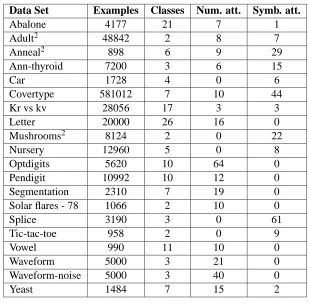
In this section, OnlineTree2 is evaluated with real problems that do not change over time. Table 2 shows a summary of twenty data sets used in this section that have been obtained from the UCI Machine Learning Repository (Asuncion and Newman, 2007). In the case of missing values, these are considered as another valid value (Quinlan, 1986). Performance of analysed algorithms is doc-umented in terms of error rate, execution time, examples stored, and false alarms triggered. This time, algorithms used to compare results with are: CVFDT, C4.5, IB1 (no window used), SMO, MLP and Na¨ıve Bayes.
The experiment was designed based on that proposed by Dietterich (1998). It can be described as follows: for each problem a) the examples are randomly distributed; b) a two fold cross validation is carried out with each learning algorithm; c) the resulting values in each fold are noted. These steps are repeated 5 times (producing a 5x2 CV), providing ten measurements for each algorithm and data set. These results were analysed using the recently proposed method by Demˇsar (2006), which focuses in comparing classifiers over multiple data sets.
The latter methodology assigns a rank to each algorithm on a data set, using its reported result based on error rates. The average rank of each algorithm is then calculated. These average values
Figure 7: Results on Electricity Market Data Set
are used to decide, with a non parametrical F test, if there is a significant difference between the algorithms. If so, the critical difference measurement (CD) is calculated using the Nemenyi test. Any difference larger than this CD when analysing a pair of algorithms confirms that they are significantly different.
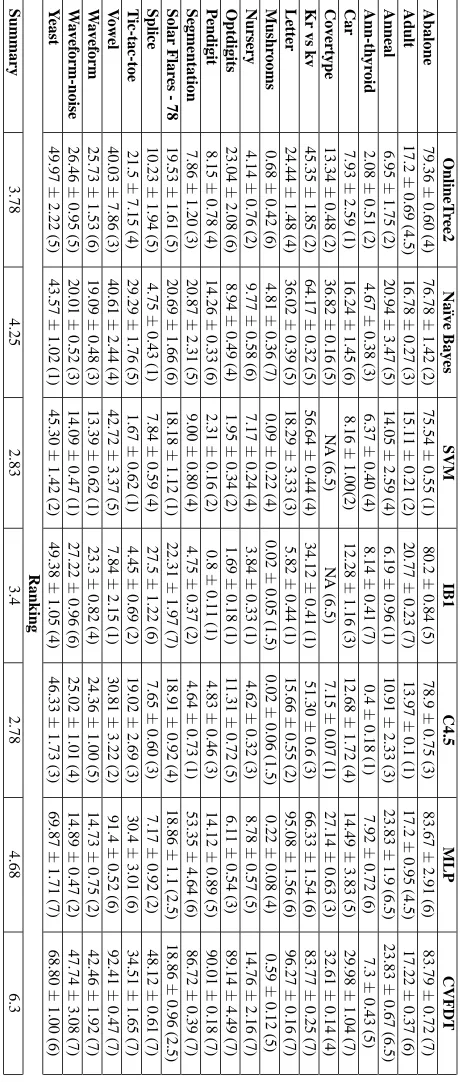
In Table 3, results on average error rate and standard deviation for each algorithm and data set are shown, as well as their ranks. Tails in average errors are solved by assigning an average of their ranks. NA error values for these measures were due to an algorithm taking more than one day to evaluate one fold of the cross validation on a data set, and the assigned rank is the largest. At the bottom of Table 3, the average of ranks for each algorithm is provided.
The Friedman test (with a significance level of 0.05) reveals that there are differences between the algorithms. Thus, a Nemenyi test (with a significance level of 0.05) is performed. The CD value for this experiment is 2.01. Figure 8 shows the critical difference diagram.
These results show that, for the data sets evaluated, there are two groups of algorithms that are not significantly different. OnlineTree2 is in the group with better ranking, and outperforms CVFDT. This demonstrates the effectiveness of Onlinetree2 in facing these kinds of problems.
Data Set Examples Classes Num. att. Symb. att.
Abalone 4177 21 7 1
Adult2 48842 2 8 7
Anneal2 898 6 9 29
Ann-thyroid 7200 3 6 15
Car 1728 4 0 6
Covertype 581012 7 10 44
Kr vs kv 28056 17 3 3
Letter 20000 26 16 0
Mushrooms2 8124 2 0 22
Nursery 12960 5 0 8
Optdigits 5620 10 64 0
Pendigit 10992 10 12 0
Segmentation 2310 7 19 0
Solar flares - 78 1066 2 10 0
Splice 3190 3 0 61
Tic-tac-toe 958 2 0 9
Vowel 990 11 10 0
Waveform 5000 3 21 0
Waveform-noise 5000 3 40 0
Yeast 1484 7 15 2
Table 2: Summary of characteristics of the evaluated data sets
Figure 8: The critical difference diagram shows two groups (bold lines) of classifiers which are not significantly different
drifting environments. Execution time of CVFDT algorithm was shorter than OnlineTree2 execution time, but, as said before, it is significantly worse than our algorithm in these evaluations.
With respect to results of OnlineTree2 regarding number of drift detected, they shown that the algorithm detects false alarms when the algorithm starts to process each data set, presumably
because of the low number of examples at that moment. Once several examples have been treated, this metric does not detect any false alarms.
In this experiment, the performance of our method is similar to that of algorithms used in analy-sis. However, it is important to note that, for each data set, the error rates achieved with OnlineTree2 have been obtained from trees which contain a reduced subset of the original data set (very small in some cases), and it is several times faster than other algorithms. Furthermore, although our method generates binary decision trees, we observed that it contains fewer leaves than the ones obtained by CVFDT and C4.5 algorithms.
6. Limitations and Future Lines
As previously mentioned OnlineTree2 is an algorithm with partial memory management, therefore its consumption of resources limits it to problems where a medium level processing capacity is avail-able. For example, for a similar data stream of that used in Section 5.1.2, OnlineTree2 takes about 30 examples per second, while CVFDT processes about 2000 examples per second and DDM+NB about 6000 examples per second. If the problem requires processing with few resources (i.e., em-bedded systems, mobile phones, PDAs) and high-rate arrival of examples, this algorithm does not prove adequate.
Even though computers over time will be faster and have more and more memory, we can imagine a future line of investigation which would optimise the algorithm presented or reuse many of the ideas for a new algorithm with a no-memory management. This can be appropriate when used with equipment with limited resources. Following this line, we think that a good contribution should be to give a more intelligent method for split numerical attributes without damage the complexity showed in Section 4.4.
With the aim of improving the precision of this algorithm, although sacrificing representation of knowledge, a Na¨ıve Bayes approach could be incorporated into the leaves as suggested by Gama et al. (2003).
7. Conclusions
An incremental decision tree learning method has been presented which is able to learn chang-ing concepts with the presence of noise and virtual drift in examples for problems with unknown conditions.
Contrary to most of the current methods, OnlineTree2 uses local adaptive windows using a new strategy which forgets examples as a result of the leaf reducing its window size when the local performance decreases.
In general, OnlineTree2 is more robust to noise than current methods, as can be seen in the SEA data set evaluation and with different levels of noise in the data stream presented in Section 5.1.2. The proposed algorithm has less error rate at the end of each context than other methods studied in problems with gradual and abrupt concept drift and noise.
This algorithm has presented a low sensibility to change in the distribution of examples of data (virtual drift), as can be observed in Sections 5.1.1 and 5.1.2.
making use of such methods is complicated for the user because they should be adjusted as dynamic of data stream changes.
Furthermore, if the studied dynamic changes over time, for example a change in distribution or noise level, the performance of the algorithms which cannot adapt their parameters may be very poor when dealing with new dynamics. For example IB1 with a large global fixed window could be adequate for gradual concept changes, but it is not adequate for faster changes, and in the same way IB1 with a small global fixed window is adequate for rapid changes and less adequate for very gradual changes or even when there is no concept change. Therefore OnlineTree2 is more suitable than current methods for problems with unknown dynamics with medium or high resource levels, which require a continual functioning.
We think that the OnlineTree2 processing speed of dozens or hundreds of examples per second, on an average personal computer, is sufficient for most applications. By using OnlineTree2, the user does not need to known the details of the algorithm and does not have to carry out any parameter configuration. On the other hand, we think that algorithms like CVFDT and DDM+NB are adequate for problems with a known dynamics and a data stream of thousands of examples per second.
With the goal that learning algorithms will be used by a wider spectrum of systems and users, we think that learning algorithms should be as simple to use as possible and that the models generated should be understandable. This has been a principal motivation in the design and evaluation of the OnlineTree2 algorithm. The way in which the knowledge is represented helps to understand both the patterns discovered in each moment and the problem itself. We consider the adaptive capacity of the internal parameters to be fundamental because it will allow them to deal with problems in the real world where you can never guarantee that the dynamic of the problem will not change over time.
Acknowledgments
The authors want to thank the editor and anonymous revisors for its useful comments and sugges-tions. This work has been partially supported by the MOISES-TA project (TIN2005-08832-C03) of the Ministry of Education and Science, Spain. The authors also thank Manuel Baena for provide us with the functional implementation of DDM algorithm used in Section 5.
Appendix A. Detailed Description of OnlineTree2 Algorithm
The aim of this appendix is to make OnlineTree2 reproducible. To do so, the algorithm appearing in Table 1 will be described in terms of functions and variables. Structural concepts for the decision tree and functions used will be defined. Notation of regular expressions is used throughout this appendix. In order to reference a variable of an object, we have used subscripts (e.g., timenoderefers
to the time of the example).
A.1 Definitions
As seen in Section 4, OnlineTree2 needs to store some information in the decision tree to process examples incrementally and efficiently. This section defines this information and identifies the place where it is stored.
As stated in Section 4.2.1, every tree node has a state used to detect concept drifts.
Definition 1 (state)
state= (i/d,per f,prev-perf,anom-time,anom-perf,pers)
where: i/d means either improvement state or degradation state, perf, prev-perf and anom-perf are current, previous and anomaly performance measures, respectively; anom-time is the anomaly time when the state enters in degradation state; and, pers counts how many examples arrived at the node when it is in degradation state (from last anomaly time).
The following defines the information contained in tree nodes.
Definition 2 (info)
in f o= (cd,ecc,state)
where: cd= (class,f rec)+is the class distribution of the examples passed through the node and not forgotten (note that is the total number of this examples), ecc is the number of examples correctly classified below the node, and state is the state of the node as defined above.
Once the information in a node has been defined, we treat tree nodes as decision nodes (d-node) and leaf nodes (l-node).
Definition 3 (d-node)
d-node= (in f o,splitting-attribute,children)
where: info contains node information as defined above, splitting-attribute is the decision attribute used to split with domain D(splitting-attribute) =V1,V2and children= (V1,node1),(V2,node2)with
node1and node2as nodes associated with d-node.
Definition 4 (l-node)
l-node= (in f o,E)
where: info contains leaf information as defined above, and E is a FIFO structure containing the examples stored in the leaf. Operations defined for E are: head(E), returns the first example added to the queue; tail(E), returns the last example added to the queue; add(E, example), adds an example to the tail of E; remove(E, i), removes i examples from the head of E; and, join(E1,E2, . . .)returns
a queue with the examples from E1,E2, . . .ordered by their time stamp. Note that the label of the
leaf can be calculated efficiently from cdl−node.
OnlineTree2(node, example): node IF not IsRevisable(node) THEN
OnlineTree2(NextNode(node, example), example)
Stage 1
ELSE
IF node is a d-node Drop(node, example) AdjustLocalWindowInDegradedLeaf (leaves(node)) Prune(node) UpdatePerformance(node) TryToReconstruct(node) (a) ELSE
UpdateLeaf (node, example) IF statenis Improvement THEN
TryToReconstruct(node) IF node is a d-node THEN
AdjustLocalWindowInImprovedLeaf (node) ENDIF ELSE AdjustLocalWindowInDegradedLeaf (node) ENDIF (b) ENDIF RETURN node ENDIF Stage 2 UpdateNode(node, example) RETURN node Stage 3
Pseudocode 1: OnlineTree2 algorithm
Definition 6 (tree) A binary decision tree is a node.
Definition 7 (example)
example= ((at,v)a,class,time)
where: a is the number of attributes in the problem, (at,v)a are a attribute-value pairs describing
the example, class is the label and time is its time stamp.
A.2 OnlineTree2 Algorithm
IsRevisable(node): boolean
RETURN not (node is a d-node∧χ2-test(cd
node,cdchildren))
Pseudocode 2: IsRevisable function
NextNode(d-node, example): node
value←value/(splitting-attribute,value)∈(at,val)a
d−node
RETURN next-child / value∈A∧(A,next-child)∈childrend−node
Pseudocode 3: NextNode procedure
A.2.1 DOWNWARDSREVISION OFSTATISTICS
As discussed in Section 4.1, the first stage of the algorithm searches either a leaf or a node that does not fit with current concept (non coherent node) in the path of current example from root to a leaf. On each visited node, a call to IsRevisable function is performed (see Pseudocode 2).
It checks the node to be a leaf or for coherence with current concept by doing aχ2test with a significance level of 0.05 (Quinlan, 1986). If this test results in a coherent node, this procedure is recursively performed with the next node depending on the value in the example for the splitting attribute (by calling the NextNode function, see Pseudocode 3). If a leaf or a non coherent node is reached, the stage ends and the next one starts.
A.2.2 TREATMENT OF ALEAF OR ANONCOHERENTNODE
As stated above, this stage tries to adjust tree structure to the dynamics of current concept in the data stream. It is divided into two parts, depending on the type of node returned by the first stage: non coherent node treatment or leaf treatment.
Non Coherent Node Treatment
Once the example reaches a non coherent node, OnlineTree2 drops the example to the correct leaf, which is updated accordingly, by calling the Drop procedure (see Pseudocode 4 and related procedures: UpdateLeaf in Pseudocode 6, Store in Pseudocode 5, UpdateStatistics in Pseudocode 7 and UpdatePerformance in Pseudocode 8).
Drop(node, example)
IF node is a l-node THEN UpdateLeaf (node, example) ELSE
Drop(NextNode(node, example), example) ENDIF
Store(leaf, example)
add(Elea f,example)
Pseudocode 5: Store procedure
UpdateLeaf (l-node, example) Store(node, example)
UpdateStatistics(node, example)
UpdatePerformance(node, timeexample)
Pseudocode 6: UpdateLeaf procedure
UpdateStatistics(node, example)
Let cdf = (class,f req)∗be the class distribution of forgotten examples after stage two.
cdnode=
(class,f req0)/(class,f req)∈cdnode∧f req0=
f req if class6=classexample
f req+1 if class=classexample
cdnode=
(class,f req0)/(class,f req)∈cdnode∧f req0=
f req if(class,∗)∈/cdf
f req−f reqf if(class,f reqf)∈cdf
IF node is a l-node THEN
eccnode= max(freq / (class,freq)∈cdnode)
ELSE
eccnode=∑(V,child)∈childrennodeeccchild
ENDIF
UpdatePerformance(node, time)
Let ianode=eccnode/nenodethe instantaneous accuracy of node, andα=7/8 the factor used
for exponential smoothing
prev-per fnode←per fnode
per fnode←α·prev-per fnode+ (1−α)·ianode
IF prev-per fnode≤per fnodeTHEN
statenode←(i,per fnode,prev-per fnode,n/a,n/a,n/a)
ELSIF node is in Improvement State THEN
statenode←(d,per fnode,prev-per fnode,time,prev-per fnode,0)
ELSE
statenode←(d,per fnode,prev-per fnode,anom-timenode,anom-per fnode,persnode+1)
ENDIF
Pseudocode 8: UpdatePerformance procedure
AdjustLocalWindowInDegradedLeaf (leaves) cdf orgotten←
FOR each l in leaves DO
IF l is in Degradation State THEN
dwl←[timehead(El),anom-timel)
d pl ←(anom-per flper fl)
f fl←min(persl·d pl,1)
lwl ←[timehead(El)+|dwl| ·f fl,tail(El)]
f el← {e f ∈El/timee f ∈/lwl}
remove(El,|f el|)
cdf orgot ← {(classi,f reqi)∗/f reqi= f reqi+|{e∈ f el/classi=label(e)}|}
ENDIF ENDFOR
Pseudocode 9: AdjustLocalWindowInDegradedLeaf procedure
Then, each leaf below the non coherent node is ordered to forget examples (see AdjustLocalWin-dowInDegradedLeaf procedure in Pseudocode 9); examples forgotten are noted to update statistics of ascendant nodes in the next stage. After that, the node is converted into a leaf with the unforgotten examples (see Pseudocode 10) and its metrics for forgetting examples are updated (see Pseudocode 8). Then a reconstruction of the pruned node is attempted (see Pseudocode 11) in order to make a coherent node for the current concept.
Leaf Treatment
Pseu-Prune(node)
Enew← join({El/l∈leaves(node)})
new-lea f ←create-l-node(Enew)
statenew−lea f ←statenode
swap(node,new-lea f)
Pseudocode 10: Prune procedure
TryToReconstruct(leaf )
Let create-decision-node: E→d-node, a function that returns a decision node with two leaves as children using the gain ratio as splitting criteria (Quinlan, 1986) from a set of examples E.
max- f req=max({f req/(class,f req)∈cdlea f})
total=nelea f
IF max- f req≤etotal−max-f reqTHEN
node←create-d-node(Elea f)
IF not IsRevisable(node) THEN
swap(lea f,node)
ENDIF ENDIF
AdjustLocalWindowInImprovedLeaf (leaf )
Let brother a node such as the parent of leaf and brother is the same.
IF nelea f·per flea f >nebrotherTHEN
remove(Elea f,1)
ENDIF
Pseudocode 12: AdjustLocalWindowInImprovedLeaf procedure
UpdateNode(d-node, example)
U pdateStatistics(d-node,example)
U pdatePer f ormance(d-node)
Pseudocode 13: UpdateNode procedure
docode 11). If there is no reconstruction, the algorithm tries to find out if the leaf has become stable, deciding to forget the oldest example of the leaf in that case, by calling the AdjustLocalWindowIn-ImprovedLeaf procedure (see Pseudocode 12).
If the leaf is not improving its performance, then an attempt to reduce its local window is per-formed (see Pseudocode 9).
A.2.3 UPWARDUPDATING OFSTATISTICS
Once stage two has finished, the algorithm starts a bottom-up process, updating the information of each visited node by calling to the UpdateNode procedure (see Pseudocode 13).
References
David Aha, Dennis Kibler, and Marc Albert. Instance-based learning algorithms. Machine Learn-ing, 6:37–66, 1991.
Arthur Asuncion and David J. Newman. UCI machine learning repository. http://www.ics.uci.edu/ mlearn/MLRepository.html, Irvine, CA: University of California, Department of Information and Computer Science, 2007.
Janez Demˇsar. Statistical comparisons of classifiers over multiple data sets. Journal of Machine Learning Research, 7:1–30, 2006.
Thomas G. Dietterich. Approximate statistical tests for comparing supervised classification learning algorithms. Neural Computation, 10(7):1895–1923, 1998.
James Dougherty, Ron Kohavi, and Mehran Sahami. Supervised and unsupervised discretization of continuous features. In Proceedings of the 20th International Conference on Machine Learning, pages 194–202, 1995.
Richard Duda and Peter Hart. Pattern Classification and Scene Analysis. Wiley-Interscience, 1973.
Floriana Esposito, Donato Malerba, and Giovanni Semeraro. A comparative analysis of methods for pruning decision trees. IEEE Transactions on Pattern Analysis and Machine Intelligence, 19 (5):476–491, 1997.
Wei Fan. Systematic data selection to mine concept-drifting data streams. In Proceedings of the 10th ACM SIGKDD International Conference on Knowledge Discovery and Data Mining, pages 128–137, 2004.
Jo ˜Ao Gama and Pedro Medas. Learning decision trees from dynamic data streams. Journal of Universal Computer Science, 11(8):1353–1366, 2005.
Jo ˜Ao Gama, Pedro Medas, Gladys Castillo, and Pedro Rodrigues. Learning with drift detection. In Proceedings of the 17th Brazilian Symposium on Artificial Intelligence, pages 286–295, 2004a.
Jo ˜Ao Gama, Pedro Medas, and Pedro Rodrigues. Learning in dynamic environments: Decision trees for data streams. Pattern Recognition in Information Systems, pages 149–158, 2004b.
Jo ˜Ao Gama, Ricardo Rocha, and Pedro Medas. Accurate decision trees for mining high-speed data streams. In Proceedings of the 9th ACM SIGKDD International Conference on Knowledge Discovery and Data Mining, pages 523–528, 2003.
Michael Harries, Claude Sammut, and Kim Horn. Extracting hidden context. Machine Learning, 32(2):101–126, 1998.
Wassily Hoeffding. Probability inequalities for sums of bounded random variables. Journal of the American Statistical Association, 58:13–30, 1963.
Geoff Hulten and Pedro Domingos. VFML – a toolkit for mining high-speed time-changing data streams. http://www.cs.washington.edu/dm/vfml/, 2003.
Geoff Hulten, Laurie Spencer, and Pedro Domingos. Mining time-changing data streams. In Pro-ceedings of the 7th ACM SIGKDD International Conference on Knowledge Discovery and Data Mining, pages 97–106, 2001.
Ralf Klinkenberg. Learning drifting concepts: Example selection vs. example weighting. Intelligent Data Analysis, 8(3):281–300, 2004.
Ralf Klinkenberg and Thorsten Joachims. Detecting concept drift with support vector machines. In Proceedings of the 17th International Conference on Machine Learning, pages 487–494, 2000.