Parallel Algorithm for Learning Optimal Bayesian Network Structure
Yoshinori Tamada∗ [email protected]
Seiya Imoto [email protected]
Satoru Miyano† [email protected]
Human Genome Center
Institute of Medical Science, The University of Tokyo 4-6-1 Shirokanedai, Minato-ku, Tokyo 108-8639, Japan
Editor: Russ Greiner
Abstract
We present a parallel algorithm for the score-based optimal structure search of Bayesian networks. This algorithm is based on a dynamic programming (DP) algorithm having O(n·2n) time and space complexity, which is known to be the fastest algorithm for the optimal structure search of networks with n nodes. The bottleneck of the problem is the memory requirement, and therefore, the algorithm is currently applicable for up to a few tens of nodes. While the recently proposed algorithm overcomes this limitation by a space-time trade-off, our proposed algorithm realizes di-rect parallelization of the original DP algorithm with O(nσ)time and space overhead calculations, whereσ>0 controls the communication-space trade-off. The overall time and space complexity is
O(nσ+12n). This algorithm splits the search space so that the required communication between in-dependent calculations is minimal. Because of this advantage, our algorithm can run on distributed memory supercomputers. Through computational experiments, we confirmed that our algorithm can run in parallel using up to 256 processors with a parallelization efficiency of 0.74, compared to the original DP algorithm with a single processor. We also demonstrate optimal structure search for a 32-node network without any constraints, which is the largest network search presented in literature.
Keywords: optimal Bayesian network structure, parallel algorithm
1. Introduction
A Bayesian network represents conditional dependencies among random variables via a directed acyclic graph (DAG). Several methods can be used to construct a DAG structure from observed data, such as score-based structure search (Heckerman et al., 1995; Friedman et al., 2000; Imoto et al., 2002), statistical hypothesis testing-based structure search (Pearl, 1988), and a hybrid of these two methods (Tsamardinos et al., 2006). In this paper, we focus on a score-based learning algorithm and formalize it as a problem to search for an optimal structure that derives the maximal (or minimal) score using a score function defined on a structure with respect to an observed data set. A score function has to be decomposed as the sum of the local score functions for each node in a network. In general, posterior probability-based score functions derived from Bayesian statistics are used. The optimal score-based structure search of Bayesian networks is known to be an NP-hard
∗. Currently at Department of Computer Science, Graduate School of Information Science and Technology, The
Uni-versity of Tokyo. 7-3-1 Hongo, Bunkyo-ku, Tokyo 113-0033, Japan. [email protected].
problem (Chickering et al., 1995). Several efficient dynamic programming (DP) algorithms have been proposed to solve such problems (Ott et al., 2004; Koivisto and Sood, 2004). Such algorithms have O(n·2n) time and space complexity, where n is the number of nodes in the network. When these algorithms are applied to real problems, the main bottleneck is bound to be the memory space requirement rather than the time requirement, because these algorithms need to store the intermediate optimal structures of all combinations of node subsets during DP steps. Because of this limitation, such algorithm can be applied to networks of only up to around 25 nodes in a typical desktop computer. Thus far, the maximum number of nodes treated in an optimal search without any constraints is 29 (Silander and Myllym¨aki, 2006). This was realized by using a 100 GB external hard disk drive as the memory space instead of using the internal memory, which is currently limited to only up to several tens of GB and in a typical desktop computer.
To overcome the above mentioned limitation, Perrier et al. (2008) proposed an algorithm to reduce the search space using structural constraints. Their algorithm searches for the optimal struc-ture on a given predefined super-strucstruc-ture, which is often available in actual problems. However, it is still important to search for a globally optimal structure because Bayesian networks find a wide range of applications. As another approach to overcome the limitation, Parviainen and Koivisto (2009) proposed a space-time trade-off algorithm that can search for a globally optimal structure with less space. From empirical results for a partial sub-problem, they showed that their algorithm is computationally feasible for up to 31 nodes. They also mentioned that their algorithm can be easily parallelized with up to 2pprocessors, where p=0,1, . . . ,n/2 is a parameter that is used to control the space-time trade-off. Using parallelization, they suggested that it might be possible to search larger-scale network structures using their algorithm. The time and space complexities of their algorithm are O(n·2n(3/2)p)and O(n·2n(3/4)p), respectively.
Of course, the memory space limitation can be overcome by simply using a computer with suf-ficient memory. The DP algorithm remains computationally feasible even for a 29-node network in terms of the time requirement. For such a purpose, a supercomputer with shared memory is required. Modern supercomputers can be equipped with several terabytes of memory space. There-fore, they can be used to search larger networks than the current 29-node network that requires 100 GB of memory. However, such supercomputers are typically very expensive and are not scalable in terms of the memory size and the number of processors. In contrast, massively parallel computers, a much cheaper type of supercomputers, make use of distributed memory; in such systems many independent computers or computation nodes are combined and linked through high-speed connec-tions. This type of supercomputers is less expensive, as mentioned, and it is scalable in terms of both the memory space and the number of processors. However the DP algorithm cannot be exe-cuted on such a distributed memory computer because it requires memory access to be performed over a wide region of data, and splitting the search space across distributed processors and storing the intermediate results in the distributed memory are not trivial problems.
our algorithm guarantees that minimal communications are required between independent parallel processors. Because of this advantage, our algorithm can be easily parallelized, and, in practice, it can run very efficiently on massively parallel computers with several hundreds of processors. An-other important feature of our algorithm is that it calculates no redundant score functions, and it can distribute the entire calculation almost equally across all processors. The main operation in our algorithm is the calculation of the score function. In practice, this feature is important to actually search for the optimal structure. The overall time and space complexity is O(nσ+12n). Our algorithm
adopts an approach opposite to that of Parviainen and Koivisto (2009) to overcome the bottleneck of the memory space problem. Although our algorithm has slightly greater space and time com-plexties, it makes it possible to realize large-scale optimal network search in practice using widely available low-cost supercomputers.
Through computational experiments, we show that our algorithm is applicable to large-scale optimal structure search. First, the scalability of the proposed algorithm to the number of proces-sors is evaluated through computational experiments with simulated data. We confirmed that the program can run efficiently in parallel using up to 256 processors (CPU cores) with a paralleliza-tion efficiency of more than 0.74 on a current supercomputer system, and acceptably using up to 512 processors with a parallelization efficiency of 0.59. Finally, we demonstrate the largest optimal Bayesian network search attempted thus far on a 32-node network with 256 processors using our proposed algorithm without any constraints and without an external hard disk drive. Our algorithm was found to complete the optimal search including the score calculation within a week.
The remainder of this paper is organized as follows. Section 2 presents an overview of the Bayesian network and the optimal search algorithm, which serves as the basis for our proposed algorithm. Section 3 describes the parallel optimal search algorithm in detail. Section 4 describes the computational experiments used for evaluating our proposed algorithm and presents the obtained results. Section 5 concludes the paper with a brief discussion. The appendix contains some proofs and corollaries related to those described in the main paper.
2. Preliminaries
In this section, we first present a brief introduction to the Bayesian network model, and then, we describe the optimal search (OS) algorithm, which is the basal algorithm that we parallelize in the proposed algorithm.
2.1 Bayesian Network
A Bayesian network is a graphical model that is used to represent a joint probability of random vari-ables. By assuming the conditional independencies among variables, the joint probability of all the variables can be represented by the simple product of the conditional probabilities. These indepen-dencies can be represented via a directed acyclic graph (DAG). In a DAG, each node corresponds to a variable and a directed edge, to the conditional dependencies among variables or to the indepen-dencies from other variables. Suppose that we have n random variables, V ={X1,X2, . . . ,Xn}. The
joint probability of variables in V is represented as
P(X1,X2, . . . ,Xn) = n
∏
j=1
where PaG(Xj)represents the set of variables that are direct parents of the j-th variable Xjin network
structure G and P(Xj|PaG(Xj)), a conditional probability for variable Xj.
A score-based Bayesian network structure search or a Bayesian network estimation problem is to search for the DAG structure fitted to the observed data, in which the fitness of the structure to the given data is measured by a score function. The score function is defined on a node and its parent set. The scores of nodes obtained by a score function are called local scores. A network score is defined simply as the sum of local scores of all nodes in a network. Using a score function, the Bayesian network structure search can be defined as a problem to find a network structure ˆG that
satisfies the following equation:
ˆ
G=arg min
G n
∑
j=1
s(Xj,PaG(Xj),X),
where s(Xj,PaG(Xj),X)is a score function s : V×2V×RN,n→Rfor node Xj given the observed
input data of an(N×n)-matrix X , where N is the number of observed samples.
2.2 Optimal Search Algorithm using Dynamic Programming
Next, we briefly introduce the OS algorithm using DP proposed by Ott et al. (2004). Our proposed algorithm is a parallelized version of this algorithm. We employ score functions described as in the original paper by Ott et al. (2004). That is, a smaller score represents better fitting of the model. Therefore, the problem becomes one of finding the structure that minimizes the score function. The optimal network structure search by DP can be regarded as an optimal permutation search problem. The algorithm consists of two-layer DP: one for obtaining the optimal choice of the parent set for each node and one for obtaining the optimal permutation of nodes. First, we introduce some definitions.
Definition 1 (Optimal local score) We define the function F : V×2V →Ras
F(v,A)def=min
B⊂As(v,B,X).
That is, F(v,A)calculates the optimal choice of the parent set from A for node v and returns its optimal local score. B⊂A represents the actual optimal choice for v, and generally, we also need to include it in the algorithm along with the score, in order to reconstruct the network structure later.
Definition 2 (Optimal network score on a permutation) Letπ:{1,2, . . . ,|A|} →A be a permu-tation on A⊂V andΠA be a set of all the permutations on A. Given a permutationπ∈ΠA, the optimal network score onπcan be described as
QA(π)def=
∑
v∈AF(v,{u∈A :π−1(u)<π−1(v)}).
Definition 3 (Optimal network score) By using QA(π) defined above, we can formalize the net-work structure search as a problem to find the optimal permutation that gives the minimal netnet-work score:
M(A)def=arg min π∈ΠAQ
Here, M(A)represents the optimal permutation that derives the minimal score of the network con-sisting of nodes in A.
Finally, the following theorem provides an algorithm to calculate F(v,A), M(A), and QA(M(A))
by DP. See Ott et al. (2004) for the proof of this theorem.
Theorem 4 (Optimal network search by DP) The functions F(v,A), M(A), and QA(M(A)) de-fined above can be respectively calculated by the following recursive formulae:
F(v,A) =min{s(v,A,X),min
a∈AF(v,A\ {a})}, (1)
M(A)(i) =
M(A\ {v∗})(i) (i<|A|)
v∗ (i=|A|) , (2)
QA(M(A)) =F(v∗,A\ {v∗}) +QA\{v∗}(M(A\ {v∗})), (3)
where
v∗=arg min
v∈A{F(v,A\ {v}) +Q
A\{v}(M(A\ {v}))}.
By applying the above equations from|A|=0 to|A|=|V|, we obtain the optimal permutationπon V and its score QV(M(V))in O(n·2n)steps.
Note that in order to reconstruct the network structure, we need to keep the optimal choice of the parent set derived in Equation (1) and the optimal permutationπ=M(A)in Equation (3) for all the combinations of A⊂V in an iterative loop for the next size of A.
3. Parallel Optimal Search Algorithm
The key to parallelizing the calculation of the optimal search algorithm by DP is splitting all the combinations of nodes in a single loop of DP for F(v,A), M(A), and QA(M(A)), given above by Equations (1), (2), and (3), respectively. Simultaneously, we need to consider how to reduce the amount of information that needs to be exchanged between processors. In the calculation of M(A), we need to obtain all the results of M(·)for one-smaller subsets of A at hand, that is, M(A\ {a})
for all a∈A. Suppose that such M(A\ {a})’s are stored in the distributed memory space, and we have collected them for calculating M(A). In order to reduce the number of communications, it would be better if we can re-use the collected results for another calculation. For example, we can calculate M(B)(|B|=|A|) in the same processor that calculates M(A)such that some of M(B\ {b})
(b∈B) overlaps M(A\ {a}). That is, if we can collect the maximal number of M(X)’s for any X such that|X|=|A| −1∧X⊂ {(A\ {a})∩(B\ {b})}, then the number of communications required for calculating M(A)and M(B)can be minimized. Theorem 7 shows how we generate such a set of combinations, and we prove that it provides the optimally minimal choice of such combinations by allowing some redundant calculations.
In addition, as is evident from Equations (1), (2), and (3), the DP algorithm basically consists of simply searching for the best choice from the candidates that derive the minimal score. Time is mainly required to calculate the score function s(v,A,X)for all the nodes and their parent com-binations. Thus, our algorithm calculates s(v,A,X)equally in independent processors without any redundant calculations for this part.
3.1 Separation of Combinations
First, we define the combination, sub-combination, and super-combination of nodes.
Definition 5 (Combination) In this paper, we refer to a set of nodes in V as a combination of nodes.
We also assume a combination of k nodes, that is, X ={x1,x2, . . . ,xk} ⊂V such that ord(xi)< ord(xj) if i< j, where ord : V →N is a function that returns the index of element v∈V . For example, suppose that V={a,b,c,d}. ord(a) =1 and ord(d) =4.
Definition 6 (Sub-/super-combination) We define C′ as a sub-combination of some combination C if C′⊂C, and C is a super-combination of C′. We say that a super-combination C is generated from C′ if C is a super-combination of C′. In addition, we say that sub-combination C′ is derived from C if C′ is a sub-combination of C. For the sake of convenience, if we do not mention about the size of a sub-/super-combination of a combination, then we assume that it refers to a one-size smaller/larger sub-/super-combination. In addition, we say that two combinations A and B share sub-combinations if
A
′∩B
′6=/0, whereA
′andB
′are sets of all the sub-combinations of A and B, respectively.We present two theorems that our algorithm relies on along with their proofs. These two theo-rems are used to split the calculation of F(v,A), M(A), and QA(M(A)); all these require the results for their sub-combinations. We show that the calculation can be split by the super-combination of
A, and it is the optimal separation of the combinations in terms of the number of communications
required.
Theorem 7 (Minimality of required sub-combinations) Let
A
be a set of combinations of nodes in V , where|A|=k>0 for A∈A
and|V|=n. If|A
|= k+kσ(σ>0∧σ+k≤n), then the minimal number of sub-combinations of length k−1 required to generate all the combinations in
A
is k+k−1σ. Let S be a combination of nodes, where|S|=k+σ. We can generate a set of combinations of length k that satisfies the former condition by deriving all the sub-combinations of length k from S.Proof Because
A
contains k+kσcombinations of length k, the number of distinct elements (nodes) involved inA
is k+σand is minimal. Therefore, the number of sub-combinations required to derivek+σ k
combinations of length k in
A
is equal to the number of possible combinations that can be generated from k+σelements, and is k+k−1σ. No more combinations can be generated from k+k−1σ sub-combinations. Therefore, it is the minimal number of required sub-combinations required to generate k+kσcombinations. A super-combination S of length k+σcontains k+σelements and can derive k+kσcombinations of length k. Therefore, S can derive
A
, and all the combinations of length k−1 derived from elements in S are the sub-combinations required to generate combinations inA
.Proof Consider the set T =V\ {v1,v2, . . . ,vσ}, where any vi ∈V , and thus, |T|=n−σ. If we
generate all the combinations of length k taken from T , then these include all the combinations of length k from nodes in V without v1, . . . ,vσ, and the number of combinations is n−kσ
. Consider a set of combinations
S
={{v1, . . . ,vσ} ∪T′ : T′⊂T∧ |T′|=k}. Here,|S|=k+σfor S∈S
and|
S
|= n−kσ. Because
S
contains all the combinations of length k without v1, . . . ,vσ and all the elements inS
contain v1, . . . ,vσ, we can generate all the combinations in V of length k from someS∈
S
by combining 0≤α≤k nodes from v1, . . . ,vσ and k−α nodes from S\ {v1, . . . ,vσ}. If we remove any S∈S
from it, then there exist combinations that cannot be generated from anotherS∈
S
becauseS
lists all the combinations except for nodes v1, . . . ,vσ. Therefore,S
is the minimal set of super-combinations required to derive all the combinations of length k from V and its size is|S
|= n−kσ. We can generate
S
by taking the first n−kσcombinations from nk combinations arranged in lexicographical order.Theorem 7 can be used to split the search space of DP using by super-combinations, and Theo-rem 8 provides the number of super-combinations required in the parallel computation for a certain size of A for M(A). From these two theorems, we can easily derive the following corollaries.
Corollary 9 (Optimal separation of combination) The DP steps used to calculate M(A) and QA(M(A))in the OS algorithm can be split into n−kσ portions by super-combinations of A with length k+σ, where |A|=k. The size of each split problem is k+kσ
and the number of required M(B) for B⊂A∧ |B|=k−1 is k+k−1σ, which is the minimal number for k+kσ combinations of M(A). Here, B is a set of sub-combinations of A. The calculation of F(v,A)can also be split based on the sub-combinations B for M(A).
The separation of M(A)by super-combinations causes some redundant calculations. The fol-lowing corollary gives the amount of such overhead calculations and the overall complexity of the algorithm.
Corollary 10 (Amount of redundant calculations) If we split the calculations of M(A)(|A|=k) using super-combinations of size k+σ(σ>0), then the number of calculations of M(A) for all A⊂V is n−kσ· k+kσ
= nk
O(nσ). Thus, as compared to the original DP steps nk
, the overhead increment of the calculations for M(A),QA(M(A)), and F(v,A)is at most O(nσ). The memory re-quirement to store the intermediate results is also dependent on the size of the sub-combinations for split calculations. Therefore, the overall time and space complexity of the algorithm is O(nσ+12n).
We present a proof in Appendix B. The parameterσ>0 can be used to control the size of split problems. Because using a large value ofσsuppresses the number of required super-combinations, the number of communications required between independent calculations is also suppressed. In-stead, the large value ofσrequires a large memory space to store the sub-combinations in a pro-cessor. Therefore,σcan be used to control the trade-off between the number of communications and the memory space requirement. Because the algorithm requires the exchange of intermediate results n−kσtimes for a loop with|A|=k and is a relatively large number, decreasing the number
Increment for
k σ=1 σ=2 σ=3
1 1 2 3
2 2 5 8
10 7 30 55
14 8 37 111
27 4 8 8
Table 1: Examples of the actual increment of various values of k andσfor n=32. The increment is largest for all cases ofσfor k=14.
Algorithm 1 Process-S(S,a,n,np)calculates the functions F(v,A), M(A), and QA(M(A))for
com-binations A derived from the given super-combination S.
Input: S⊂V : Super-combination, a∈N: size of combination to be calculated, n : total number of
nodes in the network, np: number of CPU processors (cores).
Output: F(v,B), Q(A), and M(Q(A))for all sub-combinations of S with size a, v∈A, and B= A\ {v}.
1:
A
← {A⊂S :|A|=a}2: Retrieve the local scores s(v,B,X)for B=A\ {v}(v∈A∈
A
)from the LF(v,B,n,np)-thpro-cessor.
3: Retrieve F(u,B\ {u})for u∈B(B=A\ {v},v∈A∈
A
) from the LF(u,B\ {u},n,np)-thpro-cessor.
4: Retrieve QA\{v}(M(A\ {v}))for v∈A∈
A
from the LQ(A\ {v},n,np)-th processor.
5: for each A∈
A
do6: Calculate F(v,B)for v∈A,B=A\ {v} from s(v,B) and F(v,B\ {u}) for u∈B by
Equa-tion (1).
7: Calculate M(A)and QA(M(A))from QA\{v}(M(A\ {v}))and F(v,A\ {v})by Equations (3) and (2).
8: end for
9: Store Q(A)and MA(Q(A)) (A∈
A
)in the LQ(A,n,np)-th processor.10: Store F(v,B) (B=A\ {v},A∈
A
)in the LF(v,B,n,np)-th processor.shows some examples of the actual overhead increment of the DP steps, that is, n−kσ · k+kσ
/ nk
Algorithm 2 Para-OS(V,X,s,σ,np)calculates the exactly global optimal structure of the Bayesian
network with respect to the input data X and the local score function s with npprocessors.
Input: V : set of input nodes (variables) where|V|=n, X : (N×n)-input data matrix, s(v,Pa,X): function V×2V×RN×n→Rthat returns the local Bayesian network score for variable v with
its parent set Pa⊂V w.r.t. the input data matrix X , σ∈N: size of super-combination, np:
number of CPU processors (cores).
Output: G= (V,E): optimal Bayesian network structure.
1: {Initialization}
2: Calculate F(v,/0) =s(v,/0,X)for all v∈V and store it in the LF(v,/0,n,np)-th processor.
3: Store F(v,/0)as Q{v}(M({v}))and M({v})(1) =v for all v∈V in the LQ({v},n,np)-th
proces-sor.
4: {Main Loop for size of A}
5: for a=1 to n−1 do
6: {S-phase: Execute the following for-loop on i in parallel. The{r=i mod np+1}-th
proces-sor is responsible for the(i+1)-th loop.}
7: for i=0 to n n−1a −1 do
8: v←i mod n+1
9: j← ⌊i/n⌋+1
10: Pa←m(v,RLI−1(j,n−1,a))
11: Calculate s(v,Pa,X)and store it in the local memory of the r-th processor.
12: end for
13: {Q-phase: Execute the following for-loop on i in parallel. The{r=i mod np+1}-th
pro-cessor is responsible for the(i+1)-th loop.}
14: if a+σ+1>n then
15: σ←n−a−1.
16: end if
17: for i= a+σn+1
− na+−σ1
to a+σn+1 −1 do
18: S←RLI−1(i+1,n,a+σ+1).
19: Call Process-S(S,a+1,n,np).
20: end for
21: end for
22: Construct network G= (V,E) by collecting the final sets of the parents selected in line 6 of
Process-S(·).
23: return G= (V,E).
3.2 Para-OS Algorithm
According to Theorems 7 and 8 and Corollary 9, the DP steps in Equations (1), (2), and (3) of Theorem 4 can be split by super-combinations of A. The pseudocode of the proposed algorithm is given by Algorithms 1 and 2. The former is a sub-routine of the latter main algorithm.
to store not only the local scores but also the optimal choices of parent node sets, although we do not describe this explicitly. This is required to reconstruct the optimal structure after the algorithm terminates.
In this algorithm, we need to determine which processor stores the calculated intermediate re-sults. In order to calculate this, we define some functions as given below.
Definition 11 We define function m′:N×N→Nas follows:
m′(a,b) =
a if a<b
a+1 otherwise .
Using m′(a,b), we define function m : V×2V →2V as follows:
m(v,A) ={ord−1(m′(ord(u),ord(v))): u∈A}. In addition, we define function m′−1:N×N→Nas follows:
m′−1(a,b) =
a if a<b
a−1 otherwise .
Using m′−1(a,b), we define function m−1: V×2V →2V as follows:
m−1(v,A) ={ord−1(m′−1(ord(u),ord(v))): u∈A}.
The function m(v,A)maps the combination A to a new combination in V\ {v}, and m−1(v,A)is the inverse function of m(v,A). These are used in the proposed algorithm and the following function.
Definition 12 (Calculation of processor index to store and retrieve results) We define functions
LQ: 2V×N×N→Nand LF : V×2V×N×N→Nas follows:
LQ(A,n,np)
def
= (RLI(A,n)−1)mod np+1
and
LF(v,A,n,np)
def
=
(RLI(m−1(v,A),n−1)−1)×n+ (ord(v)−1) mod np+1,
where RLI(A,n)is a function used to calculate the reverse lexicographical index (RLI) of combina-tion A taken from n objects and np, the number of processors.
Function LQ(A,n,np) locates the processor index used to store the results of M(A)and QA(M(A))
and LF(v,A,n,np), the results of F(v,A). By using RLIs, the algorithm can independently and
discontinuously generate the required combinations and processor indices for storing/retrieving of intermediate results. We use RLIs instead of ordinal lexicographical indices because the conversion between a combination and the RLI can be calculated in linear time by preparing the index table once (Tamada et al., 2011). In Algorithm 2, the inverse function RLI−1(·)is also used to reconstruct a combination from the index. See Appendix D for details of these calculations.
Q{a, b, c}(M({a, b, c}))
Q{a, b, d}(M({a, b, d}))
Q{a, c, d}(M({a, c, d}))
Q{b, c, d}(M({b, c, d}))
F(a, {b, c})
F(a, {b, d})
S = {a, b, c, d}
F(a, {c, d})
F(b, {a, c})
F(b, {a, d})
F(b, {c, d})
F(c, {a, b})
F(c, {a, d})
F(c, {b, d})
F(d, {a, b})
F(d, {a, c})
F(d, {b, c}) s(a, {b, c})
s(a, {b, d}) s(a, {c, d})
s(b, {a, c}) s(b, {a, d}) s(b, {c, d}) s(c, {a, b})
s(c, {a, d}) s(c, {b, d})
s(d, {a, b}) s(d, {a, c}) s(d, {b, c})
F(a, {b}) F(a, {c}) F(a, {d})
F(b, {a}) F(b, {c}) F(b, {d})
F(c, {a}) F(c, {b}) F(c, {d})
F(d, {a}) F(d, {b}) F(d, {c})
Calculated in S-Phase
Q{a, d}(M({a, d}))
Q{a, c}(M({a, c}))
Q{a, b}(M({a, b}))
Retrieved from other processors
Calculate in Q-Phase
F(v, Aa - 1)
F(v, Aa) Q A a+1(M(Aa+1))
Q A a(M(Aa))
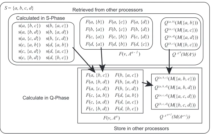
Calculation for a super-combination S = {a, b, c, d} in a single loop
Store in other processors
Q{b, c}(M({b, c}))
Figure 1: Schematic illustration of the calculation in a single loop on i for a=2. Aa represents a subset A⊂V where|A|=a.
4. Computational Experiments
In this section, we present computational experiments for evaluating the proposed algorithm. In the experiments, we first compared the running times and memory requirement for various values of σ. Next, we evaluated the running times of the original dynamic programming algorithm with a single processor and the proposed algorithm using 8 through 1024 processors. We also compared the results for different sizes of networks. In the experiments, we measured the running times using the continuous model score function BNRC proposed by Imoto et al. (2002). Finally, we tried to run the algorithm with as many nodes as possible on our supercomputers, as a proof of long-run practical execution that realizes the optimal large network structure learning. For this experiment, we used the discrete model score function BDe proposed by Heckerman et al. (1995), in addition to the BNRC score function. Brief definitions of BNRC and BDe are given in Appendix A. Before presenting the experimental results, we first describe the implementation of the algorithm and the computational environments used to execute the implemented programs.
4.1 Implementation and Computational Environment
We have used two different supercomputer systems, RIKEN RICC and Human Genome Center Supercomputer System. The former is a massively parallel computer where each computation node has dual Intel Xeon 5570 (2.93 GHz) CPUs (8 CPU cores per node) and 12 GiB memory. The computation nodes are linked by X4 DDR InfiniBand. RICC employs Fujitsu’s ParallelNavi that provides an MPI implementation, C compiler, BLAS/LAPACK library, and job scheduling. The latter system is similar to the former except that it has dual Intel Xeon 5450 (3 GHz) CPUs and 32 GiB memory per node. It employs OpenMPI 1.4 with Sun Grid Engine as a parallel computation environment. The compiler and the BLAS/LAPACK library are the Intel C compiler and Intel MKL, respectively.
In our implementation, each core in a CPU is treated equally as a single processor so that one MPI process runs in a single core. Therefore, 8 processes run in a computation node in both the systems. The memory in a single node is divided equally among these 8 processes.
For the comparison presented later and the verification of the implementation, we also imple-mented the original OS algorithm proposed by Ott et al. (2004). The verification of the implemen-tation was tested by comparing the optimal structures calculated by the implemenimplemen-tations of both the original algorithm and the proposed algorithm for up to p=23 using artificial simulated data with various numbers of processors. We also checked whether the greedy hill-climbing (HC) algorithm (Imoto et al., 2002) could search for a network structure having a better score than that of the opti-mal structure. We repeated the execution of the HC algorithm 10,000 times, and confirmed that no result was better than the optimal structure obtained using our algorithm.
4.2 Results
First, we generated artificial data with N=50 (sample size) for the randomly generated DAG struc-ture with n=23 (node size). Refer to Appendix C for details on the generation of the artificial network and data. We used n=23 because RICC has a limited running time of 72 hours. The calculation with a single processor for n=24 exceeds this limit. In all the experiments, we carried out three measurements for each setting and took the average of these measured times as an obser-vation for that setting. The total running times are measured for the entire execution of the program, including the input of the data from a file, output of the network to a file, and MPI initialization and finalization routine calls.
Figure 2 shows the result of the comparison ofσ=1, . . . ,5 for n=23. The row forσ=0 shows the results of the original DP algorithm with a single processor. We measured the running times using 256 processors here. During the computation, we also measured the times required for calling MPI functions to exchange required data between processors, and the times required for calculating the score funtion s(·). As discussed in Section 3.1,σcontrols the space-communication trade-off. We expected that an increase in the value of σwould reduce the time and increase the memory requirement. As expected, the total time decreased for up toσ=4 with an increase inσ; however, it increased for σ=5 and the memory requirement also increased significantly. As shown in the figure, σ does not affect the score calculation time. From these results, we employedσ=3 for later experiments because the increase in the memory requirement and the decrease in the total time appeared reasonable.
Next, we compared the running times for various numbers of processors. We carried out mea-surements for np =8,16,32,64,128,256,512, and 1024 processors using 1, 2, 4, 8, 16, 32, 64,
0 200 400 600 800 1000 1200 1400 1600 1800
1 2 3 4 5
10 50 100 T ime i n se co n d s Me mo ry u sa g e i n G iB σ
Total Time (left) Comm Time (left) Score Time (left) Memory (right)
σ Total Time Cm Time Sc Time Mem
0 - - - 1.27
1 1713.08 909.36 795.61 1.92 2 1267.98 458.32 794.27 4.75 3 1072.85 249.06 795.01 15.01 4 1033.20 196.04 794.75 43.69 5 1042.21 191.13 797.00 106.91
Figure 2: Running times and memory requirements withσ=1, . . . ,5 for n=23 and N=50 with 256 processors. “Total Time” represents the total time required for execution in seconds, “Cm Time” represents the total communication time required for calling MPI functions within the total time; “Sc Time,” the time required for score calculation; and “Mem,” the memory requirement in GiB.
1000 10000 100000
8 32 64 128 256 512
64 256 512 T ime i n se co n d s (l o g sca le ) Sp e e d u p
Number of processors
Time (left) Speedup (right) Ideal Speedup (right)
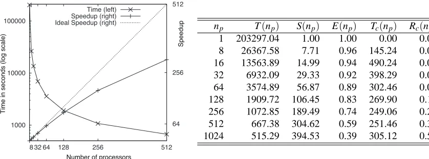
np T(np) S(np) E(np) Tc(np) Rc(np) 1 203297.04 1.00 1.00 0.00 0.00 8 26367.58 7.71 0.96 145.24 0.01 16 13563.89 14.99 0.94 490.24 0.04 32 6932.09 29.33 0.92 398.29 0.06 64 3574.89 56.87 0.89 302.46 0.08 128 1909.72 106.45 0.83 269.90 0.14 256 1072.85 189.49 0.74 249.06 0.23 512 667.38 304.62 0.59 251.46 0.38 1024 515.29 394.53 0.39 305.12 0.59
Figure 3: Scalability test results for n=23 and N =50 withσ=3. We did not present the result for np=1024 in the graph on the left-hand side because the speedup was too low.
As mentioned above, we usedσ=3. For np=1, we used the implementation of the original DP
algorithm. Therefore, we do not use the super-combination-based separation of our proposed al-gorithm although it works for np=1. Figure 3 shows the experimental result. We evaluated the
parallelization scalability of the proposed algorithm from the speedup S(np)and efficiency E(np).
100 1000 10000
20 21 22 23 24 25 26 27 10 20 30 40 50 60
T
ime
i
n
se
co
n
d
s
(l
o
g
sca
le
)
Me
mo
ry
u
sa
g
e
i
n
G
iB
(l
o
g
sca
le
)
Number of nodes
Total Time (left) Comm Time (left) Score Time (left) Memory (right)
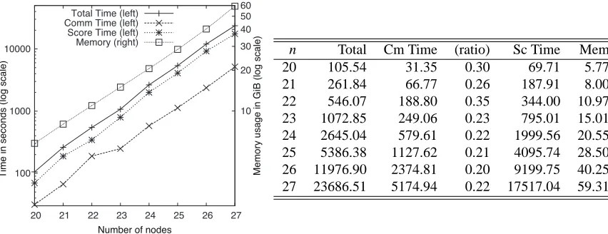
n Total Cm Time (ratio) Sc Time Mem 20 105.54 31.35 0.30 69.71 5.77 21 261.84 66.77 0.26 187.91 8.00 22 546.07 188.80 0.35 344.00 10.97 23 1072.85 249.06 0.23 795.01 15.01 24 2645.04 579.61 0.22 1999.56 20.55 25 5386.38 1127.62 0.21 4095.74 28.50 26 11976.90 2374.81 0.20 9199.75 40.25 27 23686.51 5174.94 0.22 17517.04 59.31
Figure 4: Comparison of running tims for various network sizes. Column n represents the size of the network and “(ratio),” the ratio of “Cm Time” to “Total.” “Mem” is represented in GiB. Other columns have the same meaning as in Figure 2.
that have E(np)≥0.5 are considered to be successfully parallelized. As shown in the table in
Fig-ure 3, the efficiencies are 0.74 and 0.59 for np=256 and 512, respectively. However, with 1024
processors, the efficiency became 0.39 and the speedup was very low as compared to that with 512 processors, and therefore, it is not efficient and feasible. From these results, we can conclude that the program can run very efficiently in parallel for up to 256 processors, and acceptably for up to 512 processors.
Tc(np)in Figure 3 represents the time required for calling MPI functions during the executions,
and Rc(np) is a ratio of Tc(np)to the total time T(np). Except for np=8, Tc(np) decreases with
an increase in np because the amount of communication for which each processor is responsible
decreases. However, it did not decrease linearly; in fact, for np≥512, it increased. This may
indi-cate the current limitation of both our algorithm and the computer used to carry out this experiment. For np=8, Tc(np) was very small. This is mainly because communication between computation
nodes was not required for this number of processors. If we subtract Tc(np)from T(np), then the
efficiency E(np)becomes 0.96, 0.95, and 0.94 for 256, 512, and 1024 processors, respectively. This
result suggests that the redundant calculation in our proposed algorithm does not have a great ef-fect, and the communication cost is the main cause of the inefficiency of our algorithm. Therefore, improving the communication speed in the future may significantly improve the efficiency of the algorithm with a larger number of processors.
0 2000 4000 6000 8000 10000
50 100 150 200 250 300 350 400
Time in seconds
Number of nodes Total Time
Comm Time Score Time
N Total Cm Time Sc Time 50 1072.85 249.06 795.01 100 1775.73 255.55 1492.78 150 2490.77 261.01 2201.52 200 2863.91 302.04 2533.35 250 3684.08 276.14 3379.34 300 5460.16 309.71 5122.12 350 7354.91 281.40 7045.05 400 8698.11 276.68 8392.88
Figure 5: Comparison of running times for various sample sizes. Column N represents the number of samples. Other columns have the same meaning as in Figure 2.
To check the scalability of the algorithm to the sample size, we compared the running times for various sample sizes. We generated artificial simulated data with N=50,100,150,200,250,300,350,
and 400 for the artificial network of n=23, which is used for the previous analyses. Theoretically, the sample size does not affect the running times, except for the score calculation. Figure 5 shows the result. We confirmed that the communication times are almost constant for all the tested sample sizes and that the score calculation increased with the sample sizes, as was expected. Note that the calculation of the BNRC score function is not in linear time, and it is difficult to determine the exact time complexity because it involves an iterative optimization step (Imoto et al., 2002).
4.3 Structure Search for Large Networks
Finally, we tried to search for the optimal structure of nodes with as many nodes as possible in the HGC system because it allows long execution for up to two weeks with 256 processor cores and has a larger memory in each computation node.
As in the above experiment, we first generated random DAGs having various numbers of nodes, and then generated simulated data with 50 samples. With the BNRC score function, we have suc-ceeded in searching for the optimal structure of a 31-node network by using 464.3 GiB memory in total (1.8 GiB per process) with 256 CPU cores in 32 computation nodes. For this calculation, we did not impose a restriction on the parent size or any other parameter restrictions. 8 days 6 hours 50 minutes 24 seconds were required to finish the calculation. The total time required for calling MPI functions was 2 days 15 hours 11 minutes 58 seconds. This is 32% of the total running time. Therefore, the communication time became a relatively large portion of the total computation time, relative to that in the case of n=27 presented above. As described in Parviainen and Koivisto (2009), thus far, the largest network search that has been reported was for a 29-node network (Si-lander and Myllym¨aki, 2006). Therefore, our result improved upon this result without even using an external hard disk drive.
calculated 100 times faster than the BNRC score (data not shown). Using the BDe score function, we successfully carried out optimal structure search for a 32-node network without any restriction using 836.1 GiB memory (3.3 GiB per process) in total with 256 CPU cores. The total computation time was 5 days 14 hours 24 minutes and 34 seconds. The MPI communication time was 4 days 12 hours 56 minutes 26 seconds, and this is 81% of the total time. Thus, for n=32 with the BDe score function, the calculation of score functions requires relatively very little time (actually, it required only around 1.5 hours per process) as compared to the total time, and the communication cost becomes the dominant part and the bottleneck of the calculation.
These results show that our algorithm is applicable to the optimal structure search of relatively large-sized networks and it can be run on modern low-cost supercomputers.
5. Discussions
In this paper, we have presented a parallel algorithm to search for the score-based optimal structure of Bayesian networks. The main feature of our algorithm is that it can run very efficiently on mas-sively parallel computers in parallel. We confirmed the scalability of the algorithm to the number of processors through computational experiments and successfully demonstrated optimal structure search for a 32-node network with 256 processors, an improvement over the most successful result reported thus far. Our algorithm overcomes the bottleneck of the previous algorithm by using a large amount of distributed memory for large-scale Bayesian network structure search.
Acknowledgments
Computational time was provided by the Supercomputer System, Human Genome Center, Insti-tute of Medical Science, The University of Tokyo; and RIKEN Supercomputer system, RICC. This research was supported by a Grant-in-Aid for Research and Development Project of the Next Gen-eration Integrated Simulation of Living Matter at RIKEN and by MEXT, Japan. The authors would like to thank the anonymous referees for their valuable comments.
Appendix A. Definitions of Score Functions
In this paper, we use BNRC (Imoto et al., 2002) and BDe (Heckerman et al., 1995) as a score function s(·) for computational experiments of the proposed algorithm. Here, we present brief definitions of these score functions.
A.1 The BNRC Score Function
BNRC is a score function for modeling continuous variables. In a continuous model, we consider the joint density of the variables instead of their joint probability. We search the network structure
G by maximizing the posterior of G for the input data matrix X . The posterior of G is given by
π(G|X) =π(G)
Z N
∏
i=1
n
∏
j=1
f(xi j|paGi j;θj)π(θG|λ)dθG,
whereπ(G)is the prior distribution of G; f(xi j|paGi j;θj), the local conditional density for the j-th
variable; paGi j = (pa(i1j), . . . ,pa(j)iqj), the set of observations in the i-th sample of qj variables that
represents the direct parents of the j-th node in a network;θG= (θ1, . . . ,θn), the parameter vector
of the conditional densities to be estimated; andπ(θG|λ), the prior distribution of θG specified by
the hyperparameterλ. Conditional density f(xi j|paGi j;θj)is modeled by nonparametric regression
with B-spline basis functions given by
f(xi j|paGi j;θj) =
1
q
2πσ2j exp
"
−{xi j−∑ qj
k=1mjk(pa
(j) ik )}2
2σ2j
#
,
where mjk(p(j)ik ) =∑ Mjk l=1γ
(j) lk b
(j) lk (p
(j) ik ),{b
(j)
1k(·), . . . ,b
(j)
Mjk,k(·)}is the prescribed set of Mjk B-splines;
σj, the variance, andγ(lkj), the coefficient parameters. By taking a−2 log of the posterior, the BNRC
score function for the j-th node is defined as
sBNRC(Xj,PaG(Xj),X) =−2 log n
πG j
Z N
∏
i=1
f(xi j|paGi j;θj)πj(θj|λj)dθj o
,
whereπGJ is the prior distribution of the local structure associated with the j-th node; andπj(θj|λj),
A.2 The BDe Score Function
BDe, a score function for the discrete model, can be applied to discrete (categorical) data. As in the case of BNRC, BDe also considers the posterior of G; that is,
P(G|X)∝P(G) Z
P(X|G,θ)P(θ|G)dθ,
where P(X|G,θ) is the product of local conditional probabilities (likelihood of X given G) and
P(θ|G), the prior distribution for parameters θ. In the discrete model, we employ multinomial distribution for modeling the conditional probability and the Dirichlet distribution as its prior dis-tribution. Let Xj be a discrete random variable corresponding to the j-th node, which takes one
of r values{u1, . . . ,ur}, where r is the number of categories of Xj. In this model, the conditional
probability of Xjis parameterized as
P(Xj=uk|PaG(Xj) =ujl) =θjlk,
where ujl(l=1, . . . ,rqj)is a combination of values for the parents and qj, the number of parents of
the j-th node. Note that∑rk=1θjlk=1. For the discrete model, the likelihood can be expressed as
P(X|G,θ) = n
∏
j=1
rq j
∏
l=1
r
∏
k=1 θNjlk
jlk,
where Njlkis the number of observations for the j-th node whose values equal ukin the data matrix X with respect to a combination of the parents’ observation l. Njl=∑rk=1Njlkandθdenotes a set of
parametersθjlk. For the parameter setθ, we assume the Dirichlet distribution asπ(θ|G); then, the
marginal likelihood can be described as
Z
P(X|G,θ)P(θ|G)dθ= n
∏
j=1
rq j
∏
l=1
Γ(αjl) Γ(αjl+Njl)
r
∏
k=1
Γ(αjlk+Njlk) Γ(αjlk)
,
where θ is a set of parameters; αjlk, a hyperparameter for the Dirichlet distribution; and αjl = ∑r
k=1αjlk. By taking−log of the posterior, the BDe score function for the j-th node is defined as
sBDe(Xj,PaG(Xj),X) =−logπGj −log (
rq j
∏
l=1
Γ(αjl) Γ(αjl+Njl)
r
∏
k=1
Γ(αjlk+Njlk) Γ(αjlk)
)
,
whereπGj is the prior probability of the local structure associated with the j-th node.
Appendix B. Proof of Corollary 10
Proof We prove that n−kσ· k+kσ = nk
O(nσ).
n−σ
k
·
k+σ k
= (n−σ)!
k!(n−σ−k)!·
(k+σ)!
k!(k+σ−k)!
= (n−σ)!
k!(n−σ−k)!·
(k+σ)!
k!σ! ·
(n−k)!
(n−k)!·
= n! k!(n−k)!·
(n−σ)!(k+σ)!(n−k)!
(n−σ−k)!k!σ!n!
=
n k
· (n−σ)! (n−σ−k)!·
(k+σ)!
k!σ! ·
(n−k)!
n!
=
n k
·(n−σ) n
(n−σ−1) (n−1) · · ·
(n−σ−k+1) (n−k+1) ·
(k+σ)· · ·(k+1)k!
σ!k!
=
n k
·O(1)·O((k+σ)σ) =
n k
·O((k+σ)σ).
For n<k+σ, we consider only super-combinations of size n. Thus, for each k, there are at most nkO(nσ)calculations.
Appendix C. Method for Generating Artificial Network and Data
To generate the random DAG structure, we simply added edges at random to an empty graph so that the acyclic structure is maintained and the average degree becomes d=4.0. Consequently, the number of total edges equals n·d/2. Note that the degree of DAGs does not affect the execution time of the algorithm as the algorithm searches all possible structures. To generate the artificial data, we first randomly assigned 8 different nonlinear or linear equations to the edges and then generated the artificial numerical values based on the normal distribution and the assigned equations. Figure 6 shows the assigned equations and examples of the generated data. If a node has more than two parent nodes, the generated values are summed before adding the noise. We set the noise ratio to be 0.2.
To apply BDe to the artificial data on the n=32 network, we discretized the continuous data generated by the same method for all variables into three categories (r=3) and then executed the algorithm for these discretized values.
Appendix D. Efficient Indexing of Combinations
When running the algorithm, we need to generate combination vectors discontinuously and indepen-dently in a processor. To do this efficiently, we require an algorithm that calculates a combination vector from its index and the index from its combination vector. Buckles and Lybanon (1977) pre-sented an efficient lexicographical index - vector conversion algorithm. However, this algorithm requires the calculation of binomial coefficients for every possible element in a combination every time. To speed up this calculation, we developed a linear time algorithm that needed polynomial time to construct a reusable table (Tamada et al., 2011). Our algorithm actually deals with the
re-verse lexicographical index instead of the ordinal lexicographical index; this enables us to calculate
the table only once and to make it reusable. In this section, we present the algorithms as described in Tamada et al. (2011). See Tamada et al. (2011) for details and the proofs of the theorems. In this section, note that we assume that∑ni=kfi=0 for any fiif n<k.
Theorem 13 (RLI calculation) Let
C
={C1,C2, . . . ,Cm} be the set of all the combinations of length k taken from n objects, arranged in lexicographical order, where m= nk(a) fa(X) =X+ε
(b) fb(X) =−X+ε
(c) fc(X) =1+e1−4X +ε (d) fd(X) =−1+e1−4X +ε (e) fe(X) =−(X−1.5)2+ε
(f) ff(X) = (−X−2.5)2+ε
(g) fg(X) =−(−X−2.5)2+ε
(h) fh(X) = (X−1.5)2+ε
−4 0 2
−2
0
2
4
−2 2 6
−4
0
2
4
−2 0 1 2
−4
−2
0
2
−6 −2 2 4
−3
−1
1
3
−4 0 2 4
−4
0
2
4
−6 −2 2 4
−2
0
2
4
−2 0 1 2
−4
0
2
4
−4 0 2 4 6
−4 0 2 4 (a) (b) (c) (d) (e) (f) (g) (h)
Figure 6: Left: Linear and nonlinear equations assigned to each edge in artificial networks.ε repre-sents the noise based on the normal distribution. Right: Examples of the values generated by these equations.
1,2,3 1,2,4 1,2,5 1,2,6 1,3,4 1,3,5 1,3,6 1,4,5 1,4,6 1,5,6 2,3,4 2,3,5 2,3,6 2,4,5 2,4,6 3,4,5 3,4,6 3,5,6 4,5,6 2,5,6 1 2 3 4 5 6 7 8 9 10 11 12 13 14 15 16 17 18 19 20
RLI(X, n) X
5 2
( )
4 2( )
3 2( )
= 10 = 6 = 3 2 2( )
= 1 42
( )
32
( )
22
( )
+ + =
( )
53 = 103 2
( )
2 =( )
43 = 4 2( )
+ 4 1( )
3 1( )
2 1( )
11
( )
31
( )
21
( )
11
( )
+ + =( )
42 = 62 1
( )
11
( )
+ =
( )
32 = 3Figure 7: RLI calculation for n=6 and k=3.
def
= m−i+1. Suppose that we consider a combination of natural numbers, that is, some
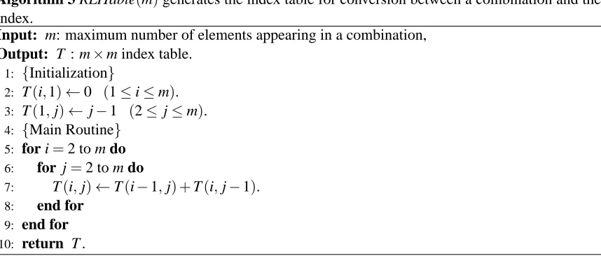
Algorithm 3 RLITable(m)generates the index table for conversion between a combination and the index.
Input: m: maximum number of elements appearing in a combination, Output: T : m×m index table.
1: {Initialization}
2: T(i,1)←0 (1≤i≤m).
3: T(1,j)← j−1 (2≤j≤m).
4: {Main Routine}
5: for i=2 to m do
6: for j=2 to m do
7: T(i,j)←T(i−1,j) +T(i,j−1).
8: end for
9: end for
10: return T .
Algorithm 4 RLI(X,n,T)calculates the reverse lexicographical index of the given combination X . Input: X={x1,x2, . . .xk} (x1<· · ·<xk∧1≤xi≤n): input combination of length k taken from
n objects, n : total number of elements, T : index table calculated by RLITable(·). Output: reverse lexicographical index of combination X .
1: r←0
2: for i=1 to k do
3: r←z+T(k−i+1,n−k−xi+i+1).
4: end for
5: return r+1.
calculated by
RLI(X,n) =
|X|
∑
i=1
n−xi |X| −i+1
+1.
Figure 7 shows an example of the calculation of RLI for n=6 and k=3. For example,
RLI({1,3,5},6) = 53 + 32
+ 11
+1=15.
Corollary 14 (RLI calculation by the index table) Let T be a(k,n−k+1)-size matrix whose ele-ment T(α,β)def= α+αβ−2
. Matrix T can be calculated only by(n−1)(n−k−1)time addition and by using T , RLI(X,n)can be calculated in linear time by RLI(X,n) =∑ki=1T(k−i+1,n−k−xi+i+1) + 1.
Algorithm 3 shows the pseudocode used to generate T and Algorithm 4, the pseudocode of
RLI(X,n). The inverse function that generates the combination vector for an RLI can be calculated by simply finding the largest column position of T , subtracting the value in the table from the index, and then repeating this k times.
Algorithm 5 RLI−1(r,n,k,T)calculates the combination vector of length k from n elements, corre-sponding to the given reverse lexicographical index r.
Input: r : reverse lexicographical index of the combination to be calculated, n : total number of elements, k : length of the combination, T : index table calculated by RLITable(·).
Output: X={x1,x2, . . . ,xk}: combination corresponding to r.
1: r←r−1.
2: for i=1 to k do
3: for j=n−k+1 to 1 do
4: if r≥T(k−i+1,j)then
5: xi←n−k−j+i+1.
6: r←r−T(k−i+1,j).
7: break
8: end if
9: end for
10: end for
11: return X={x1,x2, . . . ,xk}.
RLI−1(RLI(X,n),n,k)can be calculated by, for i=1, . . . ,k, xi=arg max
j T(k−i+1,n−k−j+i+1) <RLI(X)−
i−1
∑
α=1
T(k−α+1,n−k−xα+α+1).
Algorithm 5 shows the pseudocode used to calculate RLI−1(r,n,k)for RLI r in linear time.
The search space of 15 is independent of k but dependent on n. This is because once xi is
identified, we need to search only xj for j>i such that xj>xi. Therefore, the inverse function RLI−1(·)can generate the combination vector in linear time. By using the binary search, the search of proper objects in a vector can be calculated in log time. See Tamada et al. (2011) for the binary search version of this algorithm.
The advantage of using RLI is that once T is calculated for m, it can be used for calculating
RLI(X,n)and RLI−1(r,n,k)for any n and k, where k≤n≤m. The normal lexicographical order
can also be calculated in a similar manner for fixed values of n and k. However, it is required for constructing a different table for different values of n and k.
References
B. P. Buckles and M. Lybanon. Algorithm 515: Generation of a vector from the lexicographical index [G6]. ACM Transductions on Mathematical Software, 3(2):180–182, 1977.
D. M. Chickering, D. Geiger, and D. Heckerman. Learning Bayesian networks: Search methods and experimental results. In Proceedings of the Fifth Conference on Artificial Intelligence and
Statistics, pages 112–128, 1995.
D. Heckerman, D. Geiger, and D. M. Chickering. Learning Bayesian networks: the combination of knowledge and statistical data. Machine Learning, 20:197–243, 1995.
S. Imoto, T. Goto, and S. Miyano. Estimation of genetic networks and functional structures be-tween genes by using Bayesian networks and nonparametric regression. Pacific Symposium on
Biocomputing, 7:175–186, 2002.
M. Koivisto and K. Sood. Exact Bayesian structure discovery in Bayesian networks. Journal of
Machine Learning Research, 5:549–573, 2004.
S. Ott, S. Imoto, and S. Miyano. Finding optimal models for small gene networks. Pacific
Sympo-sium on Biocomputing, 9:557–567, 2004.
P. Parviainen and M. Koivisto. Exact structure discovery in Bayesian networks with less space.
Proceedings of the 25th Conference on Uncertainty in Artificial Intelligence (UAI 2009), 2009.
J. Pearl. Probabilistic Reasoning in Intelligent Systems: Networks of Plausible Inference. Morgan Kaufman Publishers, San Mateo, CA, 1988.
E. Perrier, S. Imoto, and S. Miyano. Finding optimal Bayesian network given a super-structure. J.
Machine Learning Research, 9:2251–2286, 2008.
T. Silander and P. Myllym¨aki. A simple approach for finding the globally optimal Bayesian network structure. Proceedings of the 22th Conference on Uncertainty in Artificial Intelligence (UAI
2006), pages 445–452, 2006.
Y. Tamada, S. Imoto, and S. Miyano. Conversion between a combination vector and the lexico-graphical index in linear time with polynomial time preprocessing, 2011. submitted.