lp-Norm Multiple Kernel Learning

ℓ

p

-Norm Multiple Kernel Learning

Marius Kloft∗ MKLOFT@CS.BERKELEY.EDU

University of California Computer Science Division Berkeley, CA 94720-1758, USA

Ulf Brefeld BREFELD@YAHOO-INC.COM

Yahoo! Research Avinguda Diagonal 177 08018 Barcelona, Spain

S¨oren Sonnenburg† SOEREN.SONNENBURG@TU-BERLIN.DE

Technische Universit¨at Berlin Franklinstr. 28/29

10587 Berlin, Germany

Alexander Zien‡ ZIEN@LIFEBIOSYSTEMS.COM

LIFE Biosystems GmbH Belfortstraße 2

69115 Heidelberg, Germany

Editor: Francis Bach

Abstract

Learning linear combinations of multiple kernels is an appealing strategy when the right choice of features is unknown. Previous approaches to multiple kernel learning (MKL) promote sparse kernel combinations to support interpretability and scalability. Unfortunately, thisℓ1-norm MKL is rarely observed to outperform trivial baselines in practical applications. To allow for robust kernel mixtures that generalize well, we extend MKL to arbitrary norms. We devise new insights on the connection between several existing MKL formulations and develop two efficient interleaved opti-mization strategies for arbitrary norms, that isℓp-norms with p_≥1. This interleaved optimization is much faster than the commonly used wrapper approaches, as demonstrated on several data sets. A theoretical analysis and an experiment on controlled artificial data shed light on the appropriateness of sparse, non-sparse andℓ∞-norm MKL in various scenarios. Importantly, empirical applications ofℓp-norm MKL to three real-world problems from computational biology show that non-sparse MKL achieves accuracies that surpass the state-of-the-art.

Data sets, source code to reproduce the experiments, implementations of the algorithms, and further information are available athttp://doc.ml.tu-berlin.de/nonsparse_mkl/.

Keywords: multiple kernel learning, learning kernels, non-sparse, support vector machine, con-vex conjugate, block coordinate descent, large scale optimization, bioinformatics, generalization bounds, Rademacher complexity

∗. Also at Machine Learning Group, Technische Universit¨at Berlin, 10587 Berlin, Germany.

†. Parts of this work were done while SS was at the Friedrich Miescher Laboratory, Max Planck Society, 72076 T¨ubingen, Germany.

1. Introduction

Kernels allow to decouple machine learning from data representations. Finding an appropriate data representation via a kernel function immediately opens the door to a vast world of powerful machine learning models (e.g., Sch¨olkopf and Smola, 2002) with many efficient and reliable off-the-shelf implementations. This has propelled the dissemination of machine learning techniques to a wide range of diverse application domains.

Finding an appropriate data abstraction—or even engineering the best kernel—for the problem at hand is not always trivial, though. Starting with cross-validation (Stone, 1974), which is probably the most prominent approach to general model selection, a great many approaches to selecting the right kernel(s) have been deployed in the literature.

Kernel target alignment (Cristianini et al., 2002; Cortes et al., 2010b) aims at learning the entries of a kernel matrix by using the outer product of the label vector as the ground-truth. Chapelle et al. (2002) and Bousquet and Herrmann (2002) minimize estimates of the generalization error of support vector machines (SVMs) using a gradient descent algorithm over the set of parameters. Ong et al. (2005) study hyperkernels on the space of kernels and alternative approaches include selecting kernels by DC programming (Argyriou et al., 2008) and semi-infinite programming ( ¨Oz¨og¨ur-Aky¨uz and Weber, 2008; Gehler and Nowozin, 2008). Although finding non-linear kernel mixtures (G¨onen and Alpaydin, 2008; Varma and Babu, 2009) generally results in non-convex optimization problems, Cortes et al. (2009b) show that convex relaxations may be obtained for special cases.

However, learning arbitrary kernel combinations is a problem too general to allow for a general optimal solution—by focusing on a restricted scenario, it is possible to achieve guaranteed optimal-ity. In their seminal work, Lanckriet et al. (2004) consider training an SVM along with optimizing the linear combination of several positive semi-definite matrices, K=∑M_m=1θmKm,subject to the

trace constraint tr(K)_≤c and requiring a valid combined kernel K 0. This spawned the new field of multiple kernel learning (MKL), the automatic combination of several kernel functions. Lanckriet et al. (2004) show that their specific version of the MKL task can be reduced to a convex optimization problem, namely a semi-definite programming (SDP) optimization problem. Though convex, however, the SDP approach is computationally too expensive for practical applications. Thus much of the subsequent research focuses on devising more efficient optimization procedures.

SVMs can still be prohibitive for large data sets. For this reason, Sonnenburg et al. (2005) also propose to interleave the SILP with the SVM training which reduces the training time drastically. Alternative optimization schemes include level-set methods (Xu et al., 2009) and second order ap-proaches (Chapelle and Rakotomamonjy, 2008). Szafranski et al. (2010), Nath et al. (2009), and Bach (2009) study composite and hierarchical kernel learning approaches. Finally, Zien and Ong (2007) and Ji et al. (2009) provide extensions for multi-class and multi-label settings, respectively.

Today, there exist two major families of multiple kernel learning models. The first is charac-terized by Ivanov regularization (Ivanov et al., 2002) over the mixing coefficients (Rakotomamonjy et al., 2007; Zien and Ong, 2007). For the Tikhonov-regularized optimization problem (Tikhonov and Arsenin, 1977), there is an additional parameter controlling the regularization of the mixing coefficients (Varma and Ray, 2007).

All the above mentioned multiple kernel learning formulations promote sparse solutions in terms of the mixing coefficients. The desire for sparse mixtures originates in practical as well as theoretical reasons. First, sparse combinations are easier to interpret. Second, irrelevant (and possibly expensive) kernels functions do not need to be evaluated at testing time. Finally, sparse-ness appears to be handy also from a technical point of view, as the additional simplex constraint kθk1≤1 simplifies derivations and turns the problem into a linearly constrained program.

Never-theless, sparseness is not always beneficial in practice and sparse MKL is frequently observed to be outperformed by a regular SVM using an unweighted-sum kernel K=∑_mKm(Cortes et al., 2008).

Consequently, despite all the substantial progress in the field of MKL, there still remains an unsatisfied need for an approach that is really useful for practical applications: a model that has a good chance of improving the accuracy (over a plain sum kernel) together with an implementation that matches today’s standards (i.e., that can be trained on 10,000s of data points in a reasonable time). In addition, since the field has grown several competing MKL formulations, it seems timely to consolidate the set of models. In this article we argue that all of this is now achievable.

1.1 Outline of the Presented Achievements

On the theoretical side, we cast multiple kernel learning as a general regularized risk minimization problem for arbitrary convex loss functions, Hilbertian regularizers, and arbitrary norm-penalties onθ. We first show that the above mentioned Tikhonov and Ivanov regularized MKL variants are equivalent in the sense that they yield the same set of hypotheses. Then we derive a dual repre-sentation and show that a variety of methods are special cases of our objective. Our optimization problem subsumes state-of-the-art approaches to multiple kernel learning, covering sparse and non-sparse MKL by arbitrary p-norm regularization (1_≤p_≤∞) on the mixing coefficients as well as the incorporation of prior knowledge by allowing for non-isotropic regularizers. As we demonstrate, the p-norm regularization includes both important special cases (sparse 1-norm and plain sum∞-norm) and offers the potential to elevate predictive accuracy over both of them.

to be stored completely in memory, which restricts these methods to small data sets with limited numbers of kernels. Our implementation is freely available within the SHOGUN machine learning toolbox available athttp://www.shogun-toolbox.org/. See also our supplementary homepage: http://doc.ml.tu-berlin.de/nonsparse_mkl/.

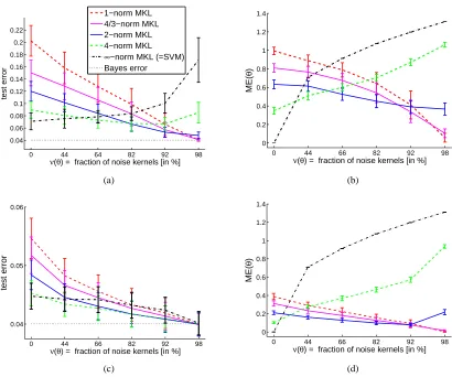
Our claims are backed up by experiments on artificial and real world data sets representing diverse, relevant and challenging problems from the application domain of bioinformatics. Using artificial data, we investigate the impact of the p-norm on the test error as a function of the size of the true sparsity pattern. The real world problems include subcellular localization of proteins, transcription start site detection, and enzyme function prediction. The results demonstrate (i) that combining kernels is now tractable on large data sets, (ii) that it can provide cutting edge classifica-tion accuracy, and (iii) that depending on the task at hand, different kernel mixture regularizaclassifica-tions are required for achieving optimal performance.

We also present a theoretical analysis of non-sparse MKL. We introduce a novel ℓ1-to-ℓp

con-version technique and use it to derive generalization bounds. Based on these, we perform a case study to compare an exemplary sparse with a non-sparse learning scenario. We show that in the sparse scenarioℓp>1-norm MKL yields a strictly better generalization bound than ℓ1-norm MKL,

while in the non-sparse scenario it is the other way around.

The remainder is structured as follows. We derive non-sparse MKL in Section 2 and discuss relations to existing approaches in Section 3. Section 4.3 introduces the novel optimization strategy and its implementation. We report on theoretical results in Section 5 and on our empirical results in Section 6. Section 7 concludes.

1.1.1 RELATED WORK

A basic version of this work appeared in NIPS 2009 (Kloft et al., 2009a). The present article additionally offers a more general and complete derivation of the main optimization problem, ex-emplary applications thereof, a simple algorithm based on a closed-form solution, technical details of the implementation, a theoretical analysis, and additional experimental results. Parts of Section 5 are based on Kloft et al. (2010) the present analysis however extends the previous publication by a novel conversion technique, an illustrative case study, tighter bounds, and an improved presentation. In related papers, non-sparse MKL has been applied, extended, and further analyzed by several researchers since its initial publication in Kloft et al. (2008), Cortes et al. (2009a), and Kloft et al. (2009a): Varma and Babu (2009) derive a projected gradient-based optimization method forℓ2-norm

MKL. Yu et al. (2010) present a more general dual view ofℓ2-norm MKL and show advantages of

ℓ2-norm over an unweighted-sum kernel SVM on six bioinformatics data sets. Cortes et al. (2010a)

provide generalization bounds for ℓ1- and ℓp≤2-norm MKL. The analytical optimization method

presented in this paper was independently and in parallel discovered by Xu et al. (2010) and has also been studied in Roth and Fischer (2007) and Ying et al. (2009) for ℓ1-norm MKL, and in

Szafranski et al. (2010) and Nath et al. (2009) for composite kernel learning on small and medium scales.

2. Multiple Kernel Learning—A Unifying View

We show that it comprises many popular MKL variants currently discussed in the literature, includ-ing seeminclud-ingly different ones.

We derive generalized dual optimization problems without making specific assumptions on the norm regularizers or the loss function, beside that the latter is convex. As a special case we derive ℓp-norm MKL in Section 4. In addition, our formulation covers binary classification and regression

tasks and can easily be extended to multi-class classification and structural learning settings using appropriate convex loss functions and joint kernel extensions (cf. Section 3). Prior knowledge on kernel mixtures and kernel asymmetries can be incorporated by non-isotropic norm regularizers.

2.1 Preliminaries

We begin with reviewing the classical supervised learning setup. Given a labeled sample

D

= {(xi,yi)}i=1...,n, where the xilie in some input space

X

and yi∈

Y

⊂R, the goal is to find a

hypoth-esis h_∈H, that generalizes well on new and unseen data. Regularized risk minimization returns a minimizer h∗,

h∗_∈argmin_hRemp(h) +λΩ(h),

where Remp(h) =1_n∑ni=1V(h(xi),yi)is the empirical risk of hypothesis h w.r.t. a convex loss function

V :R_×

Y

_→R_,Ω_{: H→}R_{is a regularizer, and}λ_{>0 is a trade-off parameter. We consider linear}

models of the form

hw˜,b(x) =hw˜,ψ(x)i+b, (1)

together with a (possibly non-linear) mappingψ:

X

_→

H

to a Hilbert space

H

(e.g., Sch¨olkopf et al., 1998; M¨uller et al., 2001) and constrain the regularization to be of the formΩ(h) = 1

2kw˜k 2 2

which allows to kernelize the resulting models and algorithms. We will later make use of kernel functions k(x,x′) =_hψ(x),ψ(x′)_iH to compute inner products in

H

.

2.2 Regularized Risk Minimization with Multiple Kernels

When learning with multiple kernels, we are given M different feature mappingsψm:

X

→

H

m,m=

1, . . .M, each giving rise to a reproducing kernel kmof

H

m. Convex approaches to multiple kernel

learning consider linear kernel mixtures kθ=∑θmkm,θm≥0. Compared to Equation (1), the primal

model for learning with multiple kernels is extended to

hw˜,b,θ(x) =

M

∑

m=1

p

θmhw˜m,ψm(x)iHm+b= hw˜,ψθ(x)iH +b

where the parameter vector ˜w and the composite feature mapψ_θhave a block structure ˜w= (w˜⊤₁, . . . , ˜

w⊤_M)⊤ andψθ=√θ1ψ1×. . .×√θMψM, respectively.

In learning with multiple kernels we aim at minimizing the loss on the training data w.r.t. the optimal kernel mixture∑M_m=1θmkmin addition to regularizingθto avoid overfitting. Hence, in terms

of regularized risk minimization, the optimization problem becomes

inf

˜ w,b,θ:θ≥0

1 n

n

∑

i=1

V

M

∑

m=1

p

θmhw˜m,ψm(xi)iHm+b, yi !

+λ 2

M

∑

m=1

for ˜µ>0. Note that the objective value of Equation (2) is an upper bound on the training error. Previous approaches to multiple kernel learning employ regularizers of the form ˜Ω(θ) =_kθ_k1 to

promote sparse kernel mixtures. In contrast, we propose to use convex regularizers of the form ˜

Ω(θ) =_kθ_k2_{, wherek · k}2 _{is an arbitrary norm in R}M_{, possibly allowing for non-sparse solutions}

and the incorporation of prior knowledge. The non-convexity arising from the√θmw˜mproduct in

the loss term of Equation (2) is not inherent and can be resolved by substituting wm←

√_θ

mw˜m.

Furthermore, the regularization parameter and the sample size can be decoupled by introducing ˜C=

1

nλ(and adjusting µ← ˜µ

λ) which has favorable scaling properties in practice. We obtain the following

convex optimization problem (Boyd and Vandenberghe, 2004) that has also been considered by Varma and Ray (2007) for hinge loss and anℓ1-norm regularizer

inf

w,b,θ:θ≥0

˜ C

n

∑

i=1

V

M

∑

m=1

hwm,ψm(xi)iHm+b, yi !

+1 2

M

∑

m=1

kwmk2_Hm

θm

+µ_kθ_k2, (3)

where we use the convention that t₀=0 if t =0 and∞otherwise.

An alternative approach has been studied by Rakotomamonjy et al. (2007) and Zien and Ong (2007), again using hinge loss andℓ1-norm. They upper bound the value of the regularizerkθk1≤1

and incorporate the regularizer as an additional constraint into the optimization problem. For C>0 and hinge loss, they arrive at the following problem which is the primary object of investigation in this paper.

2.2.1 GENERALPRIMALMKL OPTIMIZATIONPROBLEM

inf

w,b,θ:θ≥0 C n

∑

i=1

V

M

∑

m=1

hwm,ψm(xi)iHm+b, yi

+1 2

M

∑

m=1

kwmk2_H

m θm

(4)

s.t. kθk2_≤1.

It is important to note here that, while the Tikhonov regularization in (3) has two regularization pa-rameters (C and µ), the above Ivanov regularization (4) has only one (C only). Our first contribution shows that, despite the additional regularization parameter, both MKL variants are equivalent, in the sense that traversing the regularization paths yields the same binary classification functions.

Theorem 1 Let_{k · k}be a norm onRM_{and V a convex loss function. Suppose for the optimal w}∗_in Optimization Problem (4) it holds w∗₆=0. Then, for each pair(_C˜_{,µ)there exists C>0 such that} for each optimal solution (w,b,θ) of Equation (3) using(C˜,µ), we have that(w,b,κθ)is also an optimal solution of Optimization Problem (4) using C, and vice versa, whereκ>0 is a multiplicative constant.

For the proof we need Prop. 12, which justifies switching from Ivanov to Tikhonov regulariza-tion, and back, if the regularizer is tight. We refer to Appendix A for the proposition and its proof.

Proof of Theorem 1 Let be(C˜,µ)>0. In order to apply Prop. 12 to (3), we show that condition (31) in Prop. 12 is satisfied, that is, that the regularizer is tight.

Suppose on the contrary, that Optimization Problem (4) yields the same infimum regardless of whether we require

or not. Then this implies that in the optimal point we have∑M_m=1kw∗mk22

θ∗

m =0, hence,

kw∗_mk2₂

θ∗_m =0, ∀m=1, . . . ,M. (5)

Since all norms onRM _{are equivalent (e.g., Rudin, 1991), there exists a L<}∞_{such thatk}θ∗_k∞≤ Lkθ∗k. In particular, we havekθ∗k∞<∞, from which we conclude by (5), that wm=0 holds for all

m, which contradicts our assumption.

Hence, Prop. 12 can be applied,1which yields that (3) is equivalent to

inf

w,b,θ ˜ C

n

∑

i=1

V

M

∑

m=1

hwm,ψm(x)i+b,yi

+1

2

M

∑

m=1

kwmk22

θm

s.t. _kθ_k2_≤τ,

for someτ>0. Consider the optimal solution(w⋆,b⋆,θ⋆)corresponding to a given parametrization (C˜,τ). For anyλ>0, the bijective transformation(C˜,τ)_7→(λ−1/2_C˜,λτ_{)will yield(w}⋆_,b⋆_,λ1/2θ⋆₎ as optimal solution. Applying the transformation with λ:=1/τand setting C=C˜τ12 as well as κ=τ−1/2_{yields Optimization Problem (4), which was to be shown.}

Zien and Ong (2007) also show that the MKL optimization problems by Bach et al. (2004), Sonnenburg et al. (2006a), and their own formulation are equivalent. As a main implication of Theorem 1 and by using the result of Zien and Ong it follows that the optimization problem of Varma and Ray (2007) lies in the same equivalence class as Bach et al. (2004), Sonnenburg et al. (2006a), Rakotomamonjy et al. (2007) and Zien and Ong (2007). In addition, our result shows the coupling between trade-off parameter C and the regularization parameter µ in Equation (3): tweaking one also changes the other and vice versa. Theorem 1 implies that optimizing C in Optimization Problem (4) implicitly searches the regularization path for the parameter µ of Equation (3). In the remainder, we will therefore focus on the formulation in Optimization Problem (4), as a single parameter is preferable in terms of model selection.

2.3 MKL in Dual Space

In this section we study the generalized MKL approach of the previous section in the dual space. Let us begin with rewriting Optimization Problem (4) by expanding the decision values into slack variables as follows

inf

w,b,t,θ C

n

∑

i=1

V(ti,yi) +

1 2

M

∑

m=1

kwmk2_H

m θm

(6)

s.t. _∀i :

M

∑

m=1

hwm,ψm(xi)iHm+b=ti; kθk

2_{≤1 ; θ≥0,}

where_{k · k} is an arbitrary norm in Rm _{andk · kH}

M denotes the Hilbertian norm of

H

m. Applying

Lagrange’s theorem re-incorporates the constraints into the objective by introducing Lagrangian

multipliersα∈Rn_,β_∈R_{+, and}γ_∈RM_{. The Lagrangian saddle point problem is then given by}

sup

α,β,γ: β≥0,γ≥0

inf

w,b,t,θ C

n

∑

i=1

V(ti,yi) +

1 2

M

∑

m=1

kwmk2_H

m θm

−

n

∑

i=1

αi M

∑

m=1

hwm,ψm(xi)iHm+b−ti !

+β

1 2kθk

2₋1

2

−γ⊤θ.

Denoting the Lagrangian by

L

and setting its first partial derivatives with respect to w and b to 0 reveals the optimality conditions

1⊤α=0;

wm=θm n

∑

i=1

αiψm(xi), ∀m=1, . . . ,M.

Resubstituting the above equations yields

sup

α,β,γ: 1⊤α=0,

β≥0,γ≥0

inf

t,θ C

n

∑

i=1

(V(ti,yi) +αiti)−

1 2

M

∑

m=1

θmα⊤Kmα+β

1 2kθk

2

−1₂

−γ⊤θ,

which can also be written as

sup

α,β,γ: 1⊤α=0,

β≥0,γ≥0

−C

n

∑

i=1

sup

ti

−α_Citi−V(ti,yi)

−βsup

θ

1 β

M

∑

m=1

1 2α

⊤_K

mα+γm

_θ

m−

1 2kθk

2

! −1₂β.

As a consequence, we now may express the Lagrangian as2

sup

α,β,γ: 1⊤_{α=0,β≥0,γ≥0} − C

n

∑

i=1

V∗

−αi

C,yi

−_β1

1 2α ⊤_K

mα+γm

M

m=1

2 ∗ −1

2β, (7)

where h∗(x) =sup_ux⊤u₋h(u) denotes the Fenchel-Legendre conjugate of a function h and _{k ·} k∗ denotes the dual norm, that is, the norm defined via the identity 12k · k

2

∗:= 12k · k

2∗_{. In the}

following, we call V∗ the dual loss. Equation (7) now has to be maximized with respect to the dual variablesα,β, subject to 1⊤α=0 andβ≥0. Let us ignore for a moment the non-negativity constraint on β and solve ∂

L

/∂β=0 for the unboundedβ. Setting the partial derivative to zero allows to express the optimalβas

β= 1 2α ⊤_K

mα+γm

M

m=1

∗ . (8)

Obviously, at optimality, we always haveβ_≥0. We thus discard the corresponding constraint from the optimization problem and plugging Equation (8) into Equation (7) results in the following dual optimization problem:

2.3.1 GENERALDUALMKL OPTIMIZATIONPROBLEM

sup

α,γ: 1⊤_α=0,γ≥0 − C

n

∑

i=1

V∗₋αi C, yi

− 1 2α ⊤_K

mα+γm

M

m=1

∗ . (9)

The above dual generalizes multiple kernel learning to arbitrary convex loss functions and norms.3 Note that for the most common choices of norms (for example, ℓp-norm, weighted ℓp

-norms, and sum of ℓp-norms; but not the norms discussed in Section 3.5) it holdsγ∗=0 in the

optimal point so that theγ-term can be discarded and the above reduces to an optimization problem that solely depends on α. Also note that if the loss function is continuous (e.g., hinge loss), the supremum is also a maximum. The threshold b can be recovered from the solution by applying the KKT conditions.

The above dual can be characterized as follows. We start by noting that the expression in Optimization Problem (9) is a composition of two terms, first, the left hand side term, which depends on the conjugate loss function V∗, and, second, the right hand side term which depends on the conjugate norm. The right hand side can be interpreted as a regularizer on the quadratic terms that, according to the chosen norm, smoothens the solutions. Hence we have a decomposition of the dual into a loss term (in terms of the dual loss) and a regularizer (in terms of the dual norm). For a specific choice of a pair(V,_{k · k})we can immediately recover the corresponding dual by computing the pair of conjugates(V∗,_{k · k∗})(for a comprehensive list of dual losses see Rifkin and Lippert, 2007, Table 3). In the next section, this is illustrated by means of well-known loss functions and regularizers.

At this point we would like to highlight some properties of Optimization Problem (9) that arise due to our dualization technique. While approaches that firstly apply the representer theorem and secondly optimize in the primal such as Chapelle (2006) also can employ general loss functions, the resulting loss terms depend on all optimization variables. By contrast, in our formulation the dual loss terms are of a much simpler structure and they only depend on a single optimization variable αi. A similar dualization technique yielding singly-valued dual loss terms is presented in Rifkin

and Lippert (2007); it is based on Fenchel duality and limited to strictly positive definite kernel matrices. Our technique, which uses Lagrangian duality, extends the latter by allowing for positive semi-definite kernel matrices.

3. Recovering Previous MKL Formulations as Special Instances

In this section we show that existing MKL-based learners are subsumed by the generalized formu-lation in Optimization Problem (9). It is helpful for what is coming up to note that for most (but not all; see Section 3.5) choices of norms it holdsγ∗=0 in the generalized dual MKL problem (9), so that it simplifies to:

sup

α: 1⊤_α=0 − C

n

∑

i=1

V∗

−αi

C,yi

−1 2

α⊤_K mα

M

m=1

∗ . (10)

3.1 Support Vector Machines with Unweighted-Sum Kernels

First, we note that the support vector machine with an unweighted-sum kernel can be recovered as a special case of our model. To see this, we consider the regularized risk minimization problem using the hinge loss function V(t,y) =max(0,1₋ty)and the regularizer _kθ_k∞. We then can obtain the corresponding dual in terms of Fenchel-Legendre conjugate functions as follows.

We first note that the dual loss of the hinge loss is V∗(t,y) = _yt if₋1_≤ t_{y ≤}0 and∞elsewise (Rifkin and Lippert, 2007, Table 3). Hence, for each i the term V∗ ₋αi

C, yi

of the generalized dual, that is, Optimization Problem (9), translates to₋αi

Cyi, provided that 0≤

αi

yi ≤C. Employing a

variable substitution of the formαnew_i =αi

yi, Optimization Problem (9) translates to

max

α,γ:γ≥0 1 ⊤_α−

1 2α

⊤_{Y K}

mYα+γm

M

m=1

∗

, s.t. y⊤α=0 and 0_≤α_≤C1, (11)

where we denote Y =diag(y). The primalℓ_∞-norm penalty_kθ_k∞is dual to_kθ_k1, hence, via the

identity_{k · k∗}=_{k · k}1the right hand side of the last equation translates to∑mM=1α⊤Y KmYα, and we

note thatγ∗=0 in the optimal point. Combined with (11) this leads to the dual

max

α 1⊤α− M

∑

m=1

α⊤_{Y K}

mYα, s.t. y⊤α=0 and 0≤α≤C1,

which is precisely an SVM with an unweighted-sum kernel.

3.2 QCQP MKL of Lanckriet et al. (2004)

A common approach in multiple kernel learning is to employ regularizers of the form

Ω(θ) =_kθ_k1. (12)

This so-called ℓ1-norm regularizers are specific instances of sparsity-inducing regularizers. The

obtained kernel mixtures usually have a considerably large fraction of zero entries, and hence equip the MKL problem by the favor of interpretable solutions. Sparse MKL is a special case of our framework; to see this, note that the conjugate of (12) is_{k · k∞}. Recalling the definition of anℓp

-norm, the right hand side of Optimization Problem (9) translates to max_{m∈{1,...,M}}α⊤Y KmYα. The

maximum can subsequently be expanded into a slack variableξ, resulting in

sup

α,ξ

1⊤α−ξ

s.t. _∀m : 1 2α

⊤_{Y K}

mYα≤ξ; y⊤α=0 ; 0≤α≤C1,

which is the original QCQP formulation of MKL, firstly given by Lanckriet et al. (2004).

3.3 A Smooth Variant of Group Lasso

Yuan and Lin (2006) studied the following optimization problem for the special case

H

_m=Rdm_and ψm=idRdm, also known as group lasso,

min

w

C 2

n

∑

i=1

yi− M

∑

m=1

hwm,ψm(xi)iHm

!2

+1 2

M

∑

m=1

The above problem has been solved by active set methods in the primal (Roth and Fischer, 2008). We sketch an alternative approach based on dual optimization. First, we note that Equation (13) can be equivalently expressed as (Micchelli and Pontil, 2005, Lemma 26)

inf

w,θ:θ_≥0 C

2

n

∑

i=1

yi− M

∑

m=1

hwm,ψm(xi)iHm

!2

+1 2

M

∑

m=1

kwmk2_H

m θm

, s.t. _kθ_k2_1≤1.

The dual of V(t,y) = 1 2(y−t)

2 _{is V}∗_{(t,y) =} 1 2t

2_{+ty and thus the corresponding group lasso dual}

can be written as

max

α y⊤α−

1 2Ckαk

2 2− 1 2

α⊤_{Y K} mYα

M

m=1

_∞,

which can be expanded into the following QCQP

sup

α,ξ

y⊤α₋ 1 2Ckαk

2 2−ξ

s.t. _∀m : 1 2α

⊤_{Y K}

mYα≤ξ.

For small n, the latter formulation can be handled efficiently by QCQP solvers. However, the quadratic constraints caused by the non-smoothℓ_∞-norm in the objective still are computationally too demanding. As a remedy, we propose the following unconstrained variant based onℓp-norms

(1<p<∞), given by

max

α y⊤α−

1 2Ckαk

2 2− 1 2

α⊤_{Y K} mYα

M

m=1

_p∗.

It is straightforward to verify that the above objective function is differentiable in any α_∈Rn _(in

particular, notice that theℓp-norm function is differentiable for 1< p<∞) and hence the above

optimization problem can be solved very efficiently by, for example, limited memory quasi-Newton descent methods (Liu and Nocedal, 1989).

3.4 Density Level-Set Estimation

Density level-set estimators are frequently used for anomaly/novelty detection tasks (Markou and Singh, 2003a,b). Kernel approaches, such as one-class SVMs (Sch¨olkopf et al., 2001) and Sup-port Vector Domain Descriptions (Tax and Duin, 1999) can be cast into our MKL framework by employing loss functions of the form V(t) =max(0,1₋t). This gives rise to the primal

inf

w,θ:θ≥0 C n

∑

i=1

max 0,

M

∑

m=1

hwm,ψm(xi)iHm !

+1 2

M

∑

m=1

kwmk2_Hm

θm

, s.t. _kθ_k2_≤1.

Noting that the dual loss is V∗(t) =t if₋1_≤t_≤0 and∞elsewise, we obtain the following gener-alized dual

sup

α 1 ⊤_α−1

2

α⊤_K mα

M

m=1

_p∗, s.t. 0≤α≤C1,

which has been studied by Sonnenburg et al. (2006a) and Rakotomamonjy et al. (2008) forℓ1-norm,

3.5 Non-Isotropic Norms

In practice, it is often desirable for an expert to incorporate prior knowledge about the problem domain. For instance, an expert could provide estimates of the interactions of kernels_{K1, ...,KM}

in the form of an M_×M matrix E. Alternatively, E could be obtained by computing pairwise kernel alignments Ei j = _k<_KK_{ik k}i,K_Kj>_jk given a dot product on the space of kernels such as the Frobenius dot

product (Ong et al., 2005). In a third scenario, E could be a diagonal matrix encoding the a priori importance of kernels—it might be known from pilot studies that a subset of the employed kernels is inferior to the remaining ones.

All those scenarios can be handled within our framework by considering non-isotropic regular-izers of the form4

kθkE−1 = p

θ⊤_E−1θ _{with E≻0,}

where E−1is the matrix inverse of E.

However, this choice of a norm is quite different from what we have seen before: let us consider Optimization Problem (9); for non-isotropic norms we in general do not haveγ∗=0 in the optimal point so that this OP does not simplify to the dual (10) as in the subsections before. Instead we have to work with (9) directly. To this end, note that for the dual norm it holds 1_{2k · k}2_E−1

∗₌1

2k · k 2 E, so

that we obtain from (9) the following dual

sup

α,γ: 1⊤_α=0,γ≥0 − C

n

∑

i=1

V∗

−α_Ci, yi

−

1 2α

⊤_K

mα+γm

M

m=1

E

,

which is the desired non-isotropic MKL problem.

4. ℓp-Norm Multiple Kernel Learning

In this work, we propose to use non-sparse and thus more robust kernel mixtures by employing an ℓp-norm constraint with p>1, rather than the traditionally usedℓ1-norm constraint, on the mixing

coefficients (Kloft et al., 2009a). To this end, we employ non-sparse norms of the form_kθ_kp=

(∑M m=1θ

p

m)1/p, 1<p<∞.5 From the unifying framework of Section 2 we obtain the following

ℓp-norm MKL primal:

4.1 Primalℓp-norm MKL Optimization Problem

inf

w,b,θ:θ≥0 C n

∑

i=1

V

M

∑

m=1

hwm,ψm(xi)iHm+b,yi !

+1 2

M

∑

m=1

kwmk2_H

m θm

s.t. _kθ_k2_p≤1. (14)

Using that the dual norm of theℓp-norm is theℓp∗-norm, where p∗:= _pp

−1, and noting thatγ∗=0

in the optimal point, we obtain from Optimization Problem (9) the followingℓp-norm MKL dual:

4. This idea is inspired by the Mahalanobis distance (Mahalanobis, 1936).

5. While the upcoming reasoning also holds for weightedℓp-norms, the extension to more general norms, such as the

4.2 Dualℓp-norm MKL Optimization Problem

sup

α:1⊤_α=0 − C

n

∑

i=1

V∗₋αi C, yi

−1

2

α⊤_K mα

M

m=1

_p∗.

In the special case of hinge loss minimization, we obtain the optimization problem

sup

α 1 ⊤_α−1

2

α⊤_{Y K} mYα

M

m=1

p∗

, s.t. y⊤α=0 and 0_≤α_≤C1. (15)

In the subsequent sections, we will propose an efficient optimization algorithm for Optimization Problem (15) (Section 4.3) and proof its convergence (Section 4.3.3). Later we derive generalization bounds (Section 5), and analyzeℓp-norm MKL empirically using artificial and real-world data sets

(Section 6).

4.3 Optimization Strategies

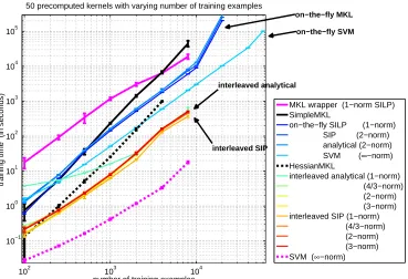
The dual as given in Optimization Problem (15) does not lend itself to efficient large-scale opti-mization in a straight-forward fashion, for instance by direct application of standard approaches like gradient descent. Instead, it is beneficial to exploit the structure of the MKL cost function by alternating between optimizing w.r.t. the mixingsθand w.r.t. the remaining variables. Most recent MKL solvers (e.g., Rakotomamonjy et al., 2008; Xu et al., 2009; Nath et al., 2009) do so by set-ting up a two-layer optimization procedure: a master problem, which is parameterized only byθ, is solved to determine the kernel mixture; to solve this master problem, repeatedly a slave prob-lem is solved which amounts to training a standard SVM on a mixture kernel. Importantly, for the slave problem, the mixture coefficients are fixed, such that conventional, efficient SVM optimizers can be recycled. Consequently these two-layer procedures are commonly implemented as wrapper approaches. Albeit appearing advantageous, wrapper methods suffer from two shortcomings: (i) Due to kernel cache limitations, the kernel matrices have to be pre-computed and stored or many kernel computations have to be carried out repeatedly, inducing heavy wastage of either memory or time. (ii) The slave problem is always optimized to the end (and many convergence proofs seem to require this), although most of the computational time is spend on the non-optimal mixtures. Cer-tainly suboptimal slave solutions would already suffice to improve far-from-optimalθin the master problem.

Due to these problems, MKL is prohibitive when learning with a multitude of kernels and on large-scale data sets as commonly encountered in many data-intense real world applications such as bioinformatics, web mining, databases, and computer security. The optimization approach pre-sented in this paper decomposes the MKL problem into smaller subproblems (Platt, 1999; Joachims, 1999; Fan et al., 2005) by establishing a wrapper-like scheme within the decomposition algorithm.

Our algorithm is embedded into the large-scale framework of Sonnenburg et al. (2006a) and extends it to the optimization of non-sparse kernel mixtures induced by anℓp-norm penalty. Our

4.3.1 A SIMPLEWRAPPERAPPROACHBASED ON ANANALYTICALUPDATE

We first present an easy-to-implement wrapper version of our optimization approach to multiple kernel learning. The interleaved decomposition algorithm is deferred to the next section.

To derive the new algorithm, we divide the optimization variables of the primal problem (14) into two groups, (w,b)on one hand and θon the other. Our algorithm will alternatingly operate on those two groups via a block coordinate descent algorithm, also known as the non-linear block Gauss-Seidel method. Thereby the optimization w.r.t. θwill be carried out analytically and the (w,b)-step will be computed in the dual, if needed.

The basic idea of our first approach is that for a given, fixed set of primal variables(w,b), the optimal θin the primal problem (14) can be calculated analytically as the following proposition shows.

Proposition 2 Let V be a convex loss function, be p>1. Given fixed (possibly suboptimal) w₆=0 and b, the minimalθin Optimization Problem (14) is attained for

θm=

kwmk

2 p+1

Hm

∑M

m′₌₁kwm′k

2p p+1

H_m′

1/p, ∀m=1, . . . ,M. (16)

Proof6 We start the derivation, by equivalently translating Optimization Problem (14) via Theo-rem 1 into

inf

w,b,θ:θ≥0

˜ C

n

∑

i=1

V

M

∑

m=1

hwm,ψm(xi)iHm+b, yi !

+1 2

M

∑

m=1

kwmk2_H

m θm

+µ 2kθk

2

p, (17)

with µ>0. Suppose we are given fixed (w,b), then setting the partial derivatives of the above objective w.r.t.θto zero yields the following condition on the optimality ofθ,

−kwmk

2

Hm

2θ2 m

+µ_·∂

1 2kθk2p

∂θm

=0, _∀m=1, . . . ,M. (18)

The first derivative of theℓp-norm with respect to the mixing coefficients can be expressed as

∂ 1

2kθk2p

∂θm

=θp−1

m kθk2p−p,

and hence Equation (18) translates into the following optimality condition,

∃ζ ∀m=1, . . . ,M : θm=ζkwmk

2 p+1

Hm . (19)

Because w₆=0, using the same argument as in the proof of Theorem 1, the constraint _kθ_k2_{p ≤}1 in (17) is at the upper bound, that is, kθkp=1 holds for an optimalθ. Inserting (19) in the latter

equation leads toζ=∑M

m=1kwmk 2p/p+1

Hm

1/p

. Resubstitution into (19) yields the claimed formula

(16).

Second, we consider how to optimize Optimization Problem (14) w.r.t. the remaining variables (w,b)for a given set of mixing coefficientsθ. Since optimization often is considerably easier in the dual space, we fixθand build the partial Lagrangian of Optimization Problem (14) w.r.t. all other primal variables w, b. The resulting dual problem is of the form (detailed derivations omitted)

sup

α:1⊤_α=0− C

n

∑

i=1

V∗₋αi C, yi

−1₂

M

∑

m=1

θmα⊤Kmα, (20)

and the KKT conditions yield wm=θm∑ni=1αiψm(xi)in the optimal point, hence

kwmk2=θ2mαKmα, ∀m=1, . . . ,M. (21)

We now have all ingredients (i.e., Equations (16), (20)–(21)) to formulate a simple macro-wrapper algorithm forℓp-norm MKL training:

Algorithm 1 Simpleℓp>1-norm MKL wrapper-based training algorithm. The analytical updates of

θand the SVM computations are optimized alternatingly. 1: input: feasibleαandθ

2: while optimality conditions are not satisfied do

3: Computeαaccording to Equation (20) (e.g., SVM)

4: Compute_kwmk2for all m=1, ...,M according to Equation (21)

5: Updateθaccording to Equation (16)

6: end while

The above algorithm alternatingly solves a convex risk minimization machine (e.g., SVM) w.r.t. the actual mixture θ(Equation (20)) and subsequently computes the analytical update according to Equation (16) and (21). It can, for example, be stopped based on changes of the objective function or the duality gap within subsequent iterations.

4.3.2 TOWARDSLARGE-SCALEMKL—INTERLEAVINGSVMANDMKL OPTIMIZATION

However, a disadvantage of the above wrapper approach still is that it deploys a full blown kernel matrix. We thus propose to interleave the SVM optimization of SVMlight with theθ- andα-steps at training time. We have implemented this so-called interleaved algorithm in Shogun for hinge loss, thereby promoting sparse solutions inα. This allows us to solely operate on a small number of active variables.7The resulting interleaved optimization method is shown in Algorithm 2. Lines 3-5 are standard in chunking based SVM solvers and carried out by SVMlight(note that Q is chosen as described in Joachims, 1999). Lines 6-7 compute SVM-objective values. Finally, the analyticalθ -step is carried out in Line 9. The algorithm terminates if the maximal KKT violation (cf. Joachims, 1999) falls below a predetermined precisionεand if the normalized maximal constraint violation |1−_ωω_old|<εmkl for the MKL-step, whereωdenotes the MKL objective function value (Line 8).

Algorithm 2 ℓp-Norm MKL chunking-based training algorithm via analytical update. Kernel

weightingθand (signed) SVMαare optimized interleavingly. The accuracy parameterεand the subproblem size Q are assumed to be given to the algorithm.

1: Initialize: gm,i=gˆi=αi=0,∀i=1, ...,n; L=S=−∞; θm= p

p

1/M,_∀m=1, ...,M 2: iterate

3: Select Q variablesαi1, . . . ,αiQ based on the gradient ˆg of (20) w.r.t.α

4: Storeαold=αand then updateαaccording to (20) with respect to the selected variables

5: Update gradient gm,i←gm,i+∑Qq=1(αiq−α

old

iq )km(xiq,xi), ∀m=1, . . . ,M, i=1, . . . ,n

6: Compute the quadratic terms Sm=1₂∑igm,iαi, qm=2θ2mSm, ∀m=1, . . . ,M

7: Lold=L, L=∑iyiαi, Sold=S, S=∑mθmSm

8: if_|1_−L L−S

old−Sold| ≥ε

9: θm= (qm)1/(p+1)/

∑M

m′=1(qm′)p/(p+1)

1/p

, ∀m=1, . . . ,M 10: else

11: break

12: end if

13: gˆi=∑mθmgm,ifor all i=1, . . . ,n

4.3.3 CONVERGENCEPROOF FORp>1

In the following, we exploit the primal view of the above algorithm as a nonlinear block Gauss-Seidel method, to prove convergence of our algorithms. We first need the following useful result about convergence of the nonlinear block Gauss-Seidel method in general.

Proposition 3 (Bertsekas, 1999, Prop. 2.7.1) Let

X

=NM_m=1

X

_mbe the Cartesian product of closed convex sets

X

m⊂Rdm, be f :

X

→Ra continuously differentiable function. Define the nonlinear

block Gauss-Seidel method recursively by letting x0_∈

X

be any feasible point, and be xk_m+1=argmin

ξ∈Xm

fxk₁+1,_···,xk_m+₋1₁,ξ,xk_m+1,_···,x_Mk , _∀m=1, . . . ,M. (22)

Suppose that for each m and x_∈

X

, the minimum

min

ξ∈Xm

f(x1,···,xm−1,ξ,xm+1,···,xM)

is uniquely attained. Then every limit point of the sequence_{xk_}k∈Nis a stationary point.

The proof can be found in Bertsekas (1999), p. 268-269. The next proposition basically establishes convergence of the proposedℓp-norm MKL training algorithm.

Theorem 4 Let V be the hinge loss and be p>1. Let the kernel matrices K1, . . . ,KM be positive

definite. Then every limit point of Algorithm 1 is a globally optimal point of Optimization Problem (14). Moreover, suppose that the SVM computation is solved exactly in each iteration, then the same holds true for Algorithm 2.

To this aim, we have to transform Optimization Problem (14) into a form such that the require-ments for application of Prop. 3 are fulfilled. We start by expanding Optimization Problem (14) into

min

w,b,ξ,θ C

n

∑

i=1

ξi+

1 2

M

∑

m=1

kwmk2Hm θm

,

s.t. _∀i :

M

∑

m=1

hwm,ψm(xi)iHm+b≥1−ξi; ξ≥0; kθk

2

p≤1; θ≥0,

thereby extending the second block of variables,(w,b), into(w,b,ξ). Moreover, we note that after an application of the representer theorem8 (Kimeldorf and Wahba, 1971) we may without loss of generality assume

H

_m=Rn_.

In the problem’s current form, the possibility of an optimal θm=0 while wm6=0 renders the

objective function nondifferentiable. This hinders the application of Prop. 3. Fortunately, it follows from Prop. 2 (note that Km≻0 implies w6=0) that this case is impossible for p>1. We therefore can

substitute the constraintθ_≥0 byθ>0 for all m without changing the optimum. In order to maintain the closeness of the feasible set we subsequently apply a bijective coordinate transformation φ:

RM

+ →RM withθnewm =φm(θm) =log(θm), resulting in the following equivalent problem,

inf

w,b,ξ,θ C

n

∑

i=1

ξi+

1 2

M

∑

m=1

exp(₋θm)kwmk2Rn,

s.t. _∀i :

M

∑

m=1

hwm,ψm(xi)iRn+b≥1−ξ_i; ξ≥0; kexp(θ)k2_p≤1,

where we employ the notation exp(θ) = (exp(θ1),···,exp(θM))⊤.

Applying the Gauss-Seidel method in Equation (22) to the base problem Optimization Problem (14) and to the reparametrized problem yields the same sequence of solutions _{(w,b,θ)k_}

k∈N₀. The above problem now allows to apply Prop. 3 for the two blocks of coordinates θ_∈

X

1 and

(w,b,ξ)_∈

X

₂: the objective is continuously differentiable and the sets

X

₁ and

X

₂ are closed and convex. To see the latter, note that_{k · k}2

p◦exp is a convex function (cf., Section 3.2.4 in Boyd and

Vandenberghe, 2004). Moreover, the minima in Equation (22) are uniquely attained: the(w,b)-step amounts to solving an SVM on a positive definite kernel mixture, and the analyticalθ-step clearly yields unique solutions as well.

Hence, we conclude that every limit point of the sequence _{(w,b,θ)k_}

k∈Nis a stationary point of Optimization Problem (14). For a convex problem, this is equivalent to such a limit point being globally optimal.

In practice, we are facing two problems. First, the standard Hilbert space setup necessarily implies that_kwmk ≥0 for all m. However in practice this assumption may often be violated, either

due to numerical imprecision or because of using an indefinite “kernel” function. However, for anykwmk ≤0 it also follows thatθ⋆m=0 as long as at least one strictly positivekwm′k>0 exists. This is because for any λ<0 we have limh_→0,h>0λ_h =−∞. Thus, for any m with kwmk ≤0, we

8. Note that the coordinate transformation into Rn _{can be explicitly given in terms of the empirical kernel map}

can immediately set the corresponding mixing coefficientsθ⋆_m to zero. The remaining θare then computed according to Equation (2), and convergence will be achieved as long as at least one strictly positive_kwm′k>0 exists in each iteration.

Second, in practice, the SVM problem will only be solved with finite precision, which may lead to convergence problems. Moreover, we actually want to improve theα only a little bit be-fore recomputingθsince computing a high precision solution can be wasteful, as indicated by the superior performance of the interleaved algorithms (cf. Sect. 6.5). This helps to avoid spending a lot ofα-optimization (SVM training) on a suboptimal mixtureθ. Fortunately, we can overcome the potential convergence problem by ensuring that the primal objective decreases within eachα-step. This is enforced in practice, by computing the SVM by a higher precision if needed. However, in our computational experiments we find that this precaution is not even necessary: even without it, the algorithm converges in all cases that we tried (cf. Section 6).

Finally, we would like to point out that the proposed block coordinate descent approach lends itself more naturally to combination with primal SVM optimizers like Chapelle (2006), LibLin-ear (Fan et al., 2008) or Ocas (Franc and Sonnenburg, 2008). Especially for linLibLin-ear kernels this is extremely appealing.

4.4 Technical Considerations

In this section we report on implementation details and discuss kernel normalization.

4.4.1 IMPLEMENTATIONDETAILS

We have implemented the analytic optimization algorithm described in the previous Section, as well as the cutting plane and Newton algorithms by Kloft et al. (2009a), within the SHOGUN toolbox (Sonnenburg et al., 2010) for regression, one-class classification, and two-class classifica-tion tasks. In addiclassifica-tion one can choose the optimizaclassifica-tion scheme, that is, decide whether the inter-leaved optimization algorithm or the wrapper algorithm should be applied. In all approaches any of the SVMs contained in SHOGUN can be used. Our implementation can be downloaded from http://www.shogun-toolbox.org.

In the more conventional family of approaches, the wrapper algorithms, an optimization scheme onθwraps around a single kernel SVM. Effectively this results in alternatingly solving forαandθ. For the outer optimization (i.e., that onθ) SHOGUN offers the three choices listed above. The semi-infinite program (SIP) uses a traditional SVM to generate new violated constraints and thus requires a single kernel SVM. A linear program (for p=1) or a sequence of quadratically constrained linear programs (for p>1) is solved via GLPK9or IBM ILOG CPLEX10. Alternatively, either an analytic or a Newton update (forℓp norms with p>1) step can be performed, obviating the need for an

additional mathematical programming software.

The second, much faster approach performs interleaved optimization and thus requires modifi-cation of the core SVM optimization algorithm. It is currently integrated into the chunking-based SVRlight and SVMlight. To reduce the implementation effort, we implement a single function perform mkl step(∑_α, obj_m), that has the arguments∑_α:=∑n

i=1αiand objm=1₂αTKmα, that is,

the current linearα-term and the SVM objectives for each kernel. This function is either, in the

9. GLPK can be found athttp://www.gnu.org/software/glpk/.

interleaved optimization case, called as a callback function (after each chunking step or a couple of SMO steps), or it is called by the wrapper algorithm (after each SVM optimization to full precision).

Recovering Regression and One-Class Classification. It should be noted that one-class classifi-cation is trivially implemented using∑_α=0 while support vector regression (SVR) is typically per-formed by internally translating the SVR problem into a standard SVM classification problem with twice the number of examples once positively and once negatively labeled with correspondingαand α∗_{. Thus one needs direct access toα}∗_{and computes∑}

α=−∑ni=1(αi+α∗i)ε−∑ni=1(αi−α∗i)yi(cf.

Sonnenburg et al., 2006a). Since this requires modification of the core SVM solver we implemented SVR only for interleaved optimization and SVMlight.

Efficiency Considerations and Kernel Caching. Note that the choice of the size of the kernel cache becomes crucial when applying MKL to large scale learning applications.11 While for the wrapper algorithms only a single kernel SVM needs to be solved and thus a single large kernel cache should be used, the story is different for interleaved optimization. Since one must keep track of the several partial MKL objectives objm, requiring access to individual kernel rows, the same

cache size should be used for all sub-kernels.

4.4.2 KERNELNORMALIZATION

The normalization of kernels is as important for MKL as the normalization of features is for training regularized linear or single-kernel models. This is owed to the bias introduced by the regularization: optimal feature / kernel weights are requested to be small. This is easier to achieve for features (or entire feature spaces, as implied by kernels) that are scaled to be of large magnitude, while down-scaling them would require a correspondingly upscaled weight for representing the same predictive model. Upscaling (downscaling) features is thus equivalent to modifying regularizers such that they penalize those features less (more). As is common practice, we here use isotropic regularizers, which penalize all dimensions uniformly. This implies that the kernels have to be normalized in a sensible way in order to represent an “uninformative prior” as to which kernels are useful.

There exist several approaches to kernel normalization, of which we use two in the computa-tional experiments below. They are fundamentally different. The first one generalizes the common practice of standardizing features to entire kernels, thereby directly implementing the spirit of the discussion above. In contrast, the second normalization approach rescales the data points to unit norm in feature space. Nevertheless it can have a beneficial effect on the scaling of kernels, as we argue below.

Multiplicative Normalization. As done in Ong and Zien (2008), we multiplicatively normalize the kernels to have uniform variance of data points in feature space. Formally, we find a positive rescalingρmof the kernel, such that the rescaled kernel ˜km(·,·) =ρmkm(·,·)and the corresponding

feature map ˜Φm(·) =√ρmΦm(·)satisfy

1 n

n

∑

i=1

_Φ˜_m(xi)−Φ˜_m(¯x)2

=1

for each m=1, . . . ,M, where ˜Φm(¯x):= 1_n∑ni=1Φ˜m(xi)is the empirical mean of the data in feature

space. The above equation can be equivalently be expressed in terms of kernel functions as

1 n

n

∑

i=1

˜km(xi,xi)−

1 n2

n

∑

i=1

n

∑

j=1

˜km(xi,xj) =1,

so that the final normalization rule is

k(x,¯x)_{7−→ 1} k(x,¯x)

n∑ n

i=1k(xi,xi)−_n12∑

n

i,j=1,k(xi,xj)

.

Note that in case the kernel is centered (i.e., the empirical mean of the data points lies on the origin), the above rule simplifies to k(x,¯x)_7−→k(x,¯x)/1_ntr(K), where tr(K):=∑n_i=1k(xi,xi) is the trace of

the kernel matrix K.

Spherical Normalization. Frequently, kernels are normalized according to

k(x,¯x)_7−→ p k(x,¯x)

k(x,x)k(¯x,¯x). (23)

After this operation,_kx_k=k(x,x) =1 holds for each data point x; this means that each data point is rescaled to lie on the unit sphere. Still, this also may have an effect on the scale of the features: a spherically normalized and centered kernel is also always multiplicatively normalized, because the multiplicative normalization rule becomes k(x,¯x)_7−→k(x,¯x)/1_ntr(K) =k(x,¯x)/1.

Thus the spherical normalization may be seen as an approximate to the above multiplicative normalization and may be used as a substitute for it. Note, however, that it changes the data points themselves by eliminating length information; whether this is desired or not depends on the learning task at hand. Finally note that both normalizations achieve that the optimal value of C is not far from 1.

4.5 Limitations and Extensions of our Framework

In this section, we show the connection ofℓp-norm MKL to a formulation based on block norms,

point out limitations and sketch extensions of our framework. To this aim let us recall the primal MKL problem (14) and consider the special case ofℓp-norm MKL given by

inf

w,b,θ:θ≥0 C n

∑

i=1

V

M

∑

m=1

hwm,ψm(xi)iHm+b,yi !

+1 2

M

∑

m=1

kwmk2_H

m θm

, s.t. _kθ_k2_p≤1. (24)

The subsequent proposition shows that (24) equivalently can be translated into the following mixed-norm formulation,

inf

w,b

˜ C

n

∑

i=1

V

M

∑

m=1

hwm,ψm(xi)iHm+b,yi !

+1 2

M

∑

m=1

kwmkq_H

m, (25)

Proposition 5 Let be p>1, be V a convex loss function, and define q := _p2p₊₁ (i.e., p= ₂₋q_q). Optimization Problem (24) and (25) are equivalent, that is, for each C there exists a ˜C>0, such that for each optimal solution (w∗,b∗,θ∗_{) of OP (24) using C, we have that (w}∗_,b∗_{) is also optimal}

in OP (25) using ˜C, and vice versa.

Proof From Prop. 2 it follows that for any fixed w in (24) it holds for the w-optimalθ:

∃ζ: θm=ζkwmk

2 p+1

Hm , ∀m=1, . . . ,M.

Plugging the above equation into (24) yields

inf

w,b C n

∑

i=1

V

M

∑

m=1

hwm,ψm(xi)iHm+b,yi !

+ 1

2ζ

M

∑

m=1

kwmk

2p p+1

Hm .

Defining q := _p2p₊₁ and ˜C :=ζC results in (25).

Now, let us take a closer look on the parameter range of q. It is easy to see that when we vary p in the real interval[1,∞], then q is limited to range in[1,2]. So in other words the methodology presented in this paper only covers the 1_≤q_≤2 block norm case. However, from an algorithmic perspective our framework can be easily extended to the q>2 case: although originally aiming at the more sophisticated case of hierarchical kernel learning, Aflalo et al. (2011) showed in particular that for q_≥2, Equation (25) is equivalent to

sup

θ:θ≥0,kθk2 r≤1

inf

w,b

˜ C

n

∑

i=1

V

M

∑

m=1

hwm,ψm(xi)iHm+b, yi !

+1 2

M

∑

m=1

θmkwmk2Hm,

where r := _q−q₂. Note the difference to ℓp-norm MKL: the mixing coefficients θ appear in the

nominator and by varying r in the interval[1,∞], the range of q in the interval[2,∞]can be obtained, which explains why this method is complementary to ours, where q ranges in[1,2].

It is straightforward to show that for every fixed (possibly suboptimal) pair(w,b)the optimalθ is given by

θm=

kwmk

2 r−1

Hm

∑M

m′₌₁kwm′k

2r r−1

H_m′

1/r, ∀m=1, . . . ,M.

The proof is analogous to that of Prop. 2 and the above analytical update formula can be used to derive a block coordinate descent algorithm that is analogous to ours. In our framework, the mixingsθ, however, appear in the denominator of the objective function of Optimization Problem (14). Therefore, the corresponding update formula in our framework is

θm=

kwmk

−2 r−1

Hm

∑M

m′₌₁kwm′k −2r r−1

H_m′

1/r, ∀m=1, . . . ,M. (26)