Importance Weighting Without Importance Weights:
An Efficient Algorithm for Combinatorial Semi-Bandits
Gergely Neu [email protected]
Universitat Pompeu Fabra
Roc Boronat 138, 08018, Barcelona, Spain
G´abor Bart´ok [email protected]
Google Z¨urich
Brandschenkestrasse 100, 8002, Z¨urich, Switzerland
Editor:Manfred Warmuth
Abstract
We propose a sample-efficient alternative for importance weighting for situations where one only has sample access to the probability distribution that generates the observations. Our new method, called Geometric Resampling (GR), is described and analyzed in the context of online combinatorial optimization under semi-bandit feedback, where a learner sequentially selects its actions from a combinatorial decision set so as to minimize its cumulative loss. In particular, we show that the well-known Follow-the-Perturbed-Leader (FPL) prediction method coupled with Geometric Resampling yields the first computationally efficient reduction from offline to online optimization in this setting. We provide a thorough theoretical analysis for the resulting algorithm, showing that its performance is on par with previous, inefficient solutions. Our main contribution is showing that, despite the relatively large variance induced by theGRprocedure, our performance guarantees hold with high probability rather than only in expectation. As a side result, we also improve the best known regret bounds forFPLin online combinatorial optimization with full feedback, closing the perceived performance gap betweenFPLand exponential weights in this setting.
Keywords: online learning, combinatorial optimization, bandit problems, semi-bandit feedback, follow the perturbed leader, importance weighting
1. Introduction
Importance weighting is a crucially important tool used in many areas of machine learning, and specifically online learning with partial feedback. While most work assumes that importance weights are readily available or can be computed with little effort during runtime, this is often not the case in many practical settings, even when one has cheap sample access to the distribution generating the observations. Among other cases, such situations may arise when observations are generated by complex hierarchical sampling schemes, probabilistic programs, or, more generally, black-box generative models. In this paper, we propose a simple and efficient sampling scheme calledGeometric Resampling (GR) to compute reliable estimates of importance weightsusing only sample access.
Our main motivation is studying a specific online learning algorithm whose practical applicability in partial-feedback settings had long been hindered by the problem outlined above. Specifically, we consider the well-known Follow-the-Perturbed-Leader (FPL) prediction method that maintains implicit sampling distributions that usually cannot be expressed in closed form. In this paper, we endow FPL with our Geometric Resampling scheme to construct the first known computationally efficient reduction from offline to online combinatorial optimization under an important
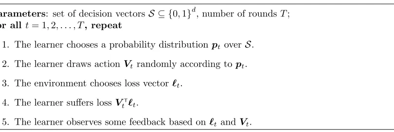
Parameters: set of decision vectorsS ⊆ {0,1}d, number of roundsT; For all t= 1,2, . . . , T, repeat
1. The learner chooses a probability distribution ptoverS.
2. The learner draws action Vtrandomly according to pt.
3. The environment chooses loss vector `t.
4. The learner suffers loss VT
t`t.
5. The learner observes some feedback based on`tand Vt.
Figure 1: The protocol of online combinatorial optimization.
information scheme known as semi-bandit feedback. In the rest of this section, we describe our precise setting, present related work and outline our main results.
1.1 Online Combinatorial Optimization
We consider a special case of online linear optimization known as online combinatorial optimization (see Figure 1). In every roundt= 1,2, . . . , T of this sequential decision problem, the learner chooses an action Vt from the finite action set S ⊆ {0,1}d, where kvk1 ≤m holds for all v ∈ S. At the same time, the environment fixes a loss vector `t ∈ [0,1]d and the learner suffers loss VtT`t. The goal of the learner is to minimize the cumulative lossPT
t=1VtT`t. As usual in the literature of online optimization (Cesa-Bianchi and Lugosi, 2006), we measure the performance of the learner in terms of theregret defined as
RT = max v∈S
T
X
t=1
(Vt−v)T`t= T
X
t=1
VT
t`t−min v∈S
T
X
t=1
vT`
t, (1)
that is, the gap between the total loss of the learning algorithm and the best fixed decision in hind-sight. In the current paper, we focus on the case ofnon-oblivious (oradaptive) environments, where we allow the loss vector`tto depend on the previous decisionsV1, . . . ,Vt−1in an arbitrary fashion. Since it is well-known that no deterministic algorithm can achieve sublinear regret under such weak assumptions, we will consider learning algorithms that choose their decisions in a randomized way. For such learners, another performance measure that we will study is theexpected regret defined as
b
RT = max v∈S
T
X
t=1
E(Vt−v)T`t=E
" T
X
t=1
VT
t`t
#
−min v∈SE
" T
X
t=1
vT`
t
#
.
The framework described above is general enough to accommodate a number of interesting problem instances such as path planning, ranking and matching problems, finding minimum-weight spanning trees and cut sets. Accordingly, different versions of this general learning problem have drawn considerable attention in the past few years. These versions differ in the amount of information made available to the learner after each roundt. In the simplest setting, called thefull-information setting, it is assumed that the learner gets to observe the loss vector `tregardless of the choice of
learner only observes the components `t,i of the loss vector for which Vt,i = 1, that is, the losses associated with the components selected by the learner.1
1.2 Related Work
The most well-known instance of our problem is the multi-armed bandit problem considered in the seminal paper of Auer, Cesa-Bianchi, Freund, and Schapire (2002): in each round of this problem, the learner has to select one ofN arms and minimize regret against the best fixed arm while only observing the losses of the chosen arms. In our framework, this setting corresponds to settingd=N andm= 1. Among other contributions concerning this problem, Auer et al. propose an algorithm called Exp3 (Exploration and Exploitation using Exponential weights) based on constructing loss estimates b`t,i for each component of the loss vector and playing arm i with probability propor-tional to exp(−ηPt−1
s=1`bs,i) at time t, where η >0 is a parameter of the algorithm, usually called
the learning rate2. This algorithm is essentially a variant of the Exponentially Weighted Average (EWA) forecaster (a variant of weighted majority algorithm of Littlestone and Warmuth, 1994, and aggregating strategies of Vovk, 1990, also known asHedge by Freund and Schapire, 1997). Besides proving that theexpected regret of Exp3isO √N TlogN, Auer et al. also provide a general lower bound of Ω √N T
on the regret of any learning algorithm on this particular problem. This lower bound was later matched by a variant of the Implicitly Normalized Forecaster (INF) of Audibert and Bubeck (2010) by using the same loss estimates in a more refined way. Audibert and Bubeck also show bounds ofO pN T /logNlog(N/δ)
on the regret that hold with probability at least 1−δ, uniformly for anyδ >0.
The most popular example of online learning problems with actual combinatorial structure is the shortest path problem first considered by Takimoto and Warmuth (2003) in the full informa-tion scheme. The same problem was considered by Gy¨orgy, Linder, Lugosi, and Ottucs´ak (2007), who proposed an algorithm that works with semi-bandit information. Since then, we have come a long way in understanding the “price of information” in online combinatorial optimization—see Audibert, Bubeck, and Lugosi (2014) for a complete overview of results concerning all of the infor-mation schemes considered in the current paper. The first algorithm directly targeting general online combinatorial optimization problems is due to Koolen, Warmuth, and Kivinen (2010): their method namedComponent Hedgeguarantees an optimal regret ofO mpTlog(d/m)in the full information setting. As later shown by Audibert, Bubeck, and Lugosi (2014), this algorithm is an instance of a more general algorithm class known as Online Stochastic Mirror Descent (OSMD). Taking the idea one step further, Audibert, Bubeck, and Lugosi (2014) also show thatOSMD-based methods can also be used for proving expected regret bounds ofO √mdTfor the semi-bandit setting, which is also shown to coincide with the minimax regret in this setting. For completeness, we note that theEWA
forecaster is known to attain an expected regret of O m3/2p
Tlog(d/m)
in the full information case andO mpdTlog(d/m)
in the semi-bandit case.
While the results outlined above might suggest that there is absolutely no work left to be done in the full information and semi-bandit schemes, we get a different picture if we restrict our attention tocomputationally efficient algorithms. First, note that methods based on exponential weighting of each decision vector can only be efficiently implemented for a handful of decision setsS—see Koolen et al. (2010) and Cesa-Bianchi and Lugosi (2012) for some examples. Furthermore, as noted by Audibert et al. (2014),OSMD-type methods can be efficiently implemented by convex programming if the convex hull of the decision set can be described by a polynomial number of constraints. Details of such an efficient implementation are worked out by Suehiro, Hatano, Kijima, Takimoto, and Nagano (2012), whose algorithm runs inO(d6) time, which can still be prohibitive in practical applications.
1 Here,Vt,iand`t,iare theithcomponents of the vectorsVt and`t, respectively.
While Koolen et al. (2010) list some further examples whereOSMD can be implemented efficiently, we conclude that there is no general efficient algorithm with near-optimal performance guarantees for learning in combinatorial semi-bandits.
The Follow-the-Perturbed-Leader (FPL) prediction method (first proposed by Hannan, 1957 and later rediscovered by Kalai and Vempala, 2005) offers a computationally efficient solution for the online combinatorial optimization problem given that thestaticcombinatorial optimization problem minv∈SvT`admits computationally efficient solutions for any `∈Rd. The idea underlying FPLis very simple: in every round t, the learner draws some random perturbationsZt∈ Rd and selects
the action that minimizes the perturbed total losses:
Vt= arg min v∈S
vT
t−1
X
s=1
`s−Zt
!
.
Despite its conceptual simplicity and computational efficiency, FPLhave been relatively overlooked until very recently, due to two main reasons:
• The best known bound for FPLin the full information setting is O m√dT, which is worse than the bounds for bothEWAandOSMDthat scale only logarithmically withd.
• Considering bandit information, no efficientFPL-style algorithm is known to achieve a regret of O √T
. On one hand, it is relatively straightforward to proveO T2/3
bounds on the expected regret for an efficientFPL-variant (see, e.g., Awerbuch and Kleinberg, 2004 and McMahan and Blum, 2004). Poland (2005) proved bounds ofO √N TlogN
in theN-armed bandit setting, however, the proposed algorithm requires O T2numerical operations per round.
The main obstacle for constructing a computationally efficientFPL-variant that works with partial information is precisely the lack of closed-form expressions for importance weights. In the current paper, we address the above two issues and show that an efficientFPL-based algorithm using inde-pendent exponentially distributed perturbations can achieve as good performance guarantees asEWA
in online combinatorial optimization.
Our work contributes to a new wave of positive results concerning FPL. Besides the reservations towardsFPLmentioned above, the reputation of FPLhas been also suffering from the fact that the nature of regularization arising from perturbations is not as well-understood as the explicit regu-larization schemes underlyingOSMD orEWA. Very recently, Abernethy et al. (2014) have shown that
FPLimplements a form of strongly convex regularization over the convex hull of the decision space. Furthermore, Rakhlin et al. (2012) showed thatFPLrun with a specific perturbation scheme can be regarded as a relaxation of the minimax algorithm. Another recently initiated line of work shows that intuitive parameter-free variants of FPL can achieve excellent performance in full-information settings (Devroye et al., 2013 and Van Erven et al., 2014).
1.3 Our Results
In this paper, we propose a loss-estimation scheme called Geometric Resampling to efficiently com-pute importance weights for the observed components of the loss vector. Building on this technique and theFPLprinciple, resulting inan efficient algorithm for regret minimization under semi-bandit feedback. Besides this contribution, our techniques also enable us to improve the best known regret bounds of FPLin the full information case. We prove the following results concerning variants of our algorithm:
• a bound of O mpdTlog(d/m)
on the expected regret under semi-bandit feedback (Theo-rem 1),
• a bound ofO mpdTlog(d/m) +√mdTlog(1/δ)
• a bound ofO m3/2p
Tlog(d/m)
on the expected regret under full information (Theorem 13).
We also show that both of our semi-bandit algorithms access the optimization oracle O(dT) times overT rounds with high probability, increasing the running time only by a factor ofdcompared to the full-information variant. Notably, our results close the gaps between the performance bounds of
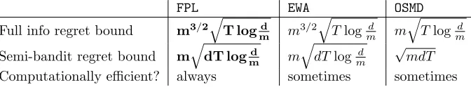
FPLandEWAunder both full information and semi-bandit feedback. Table 1 puts our newly proven regret bounds into context.
FPL EWA OSMD
Full info regret bound m3/2qT logd
m m
3/2qTlog d m m
q
Tlog d m
Semi-bandit regret bound m
q
dT logmd m
q
dTlogmd √mdT Computationally efficient? always sometimes sometimes
Table 1: Upper bounds on the regret of various algorithms for online combinatorial optimization, up to constant factors. The third row roughly describes the computational efficiency of each algorithm—see the text for details. New results are presented in boldface.
2. Geometric Resampling
In this section, we introduce the main idea underlying Geometric Resampling in the specific context ofN-armed bandits whered=N,m= 1 and the learner has access to the basis vectors{ei}di=1 as its decision set S. In this setting, components of the decision vector are referred to as arms. For ease of notation, define It as the unique arm such that Vt,It = 1 and Ft−1 as the sigma-algebra
induced by the learner’s actions and observations up to the end of roundt−1. Using this notation, we definept,i=P[It=i| Ft−1].
Most bandit algorithms rely on feeding some loss estimates to a sequential prediction algorithm. It is commonplace to considerimportance-weighted loss estimates of the form
b
`∗t,i= I{It=i}
pt,i
`t,i (2)
for allt, isuch thatpt,i >0. It is straightforward to show thatb`∗t,iis an unbiased estimate of the loss
`t,i for all such t, i. Otherwise, whenpt,i= 0, we setb`∗t,i= 0, which givesE h
b
`∗t,i
Ft−1
i
= 0≤`t,i. To our knowledge, all existing bandit algorithms operating in the non-stochastic setting utilize some version of the importance-weighted loss estimates described above. This is a very natural choice for algorithms that operate by first computing the probabilitiespt,i and then samplingIt from the resulting distributions. While many algorithms fall into this class (including the Exp3 algorithm of Auer et al. (2002), the Green algorithm of Allenberg et al. (2006) and the INF algorithm of Audibert and Bubeck (2010), one can think of many other algorithms where the distributionpt is specified implicitly and thus importance weights are not readily available. Arguably,FPLis the most important online prediction algorithm that operates with implicit distributions that are notoriously difficult to compute in closed form. To overcome this difficulty, we propose a different loss estimate that can be efficiently computedeven when ptis not available for the learner.
Our estimation procedure dubbed Geometric Resampling (GR) is based on the simple observation that, even thoughpt,Itmight not be computable in closed form, one can simply generate a geometric
random variable with expectation 1/pt,It by repeated sampling frompt. Specifically, we propose the
Geometric Resampling for multi-armed bandits
1. The learner drawsIt∼pt.
2. Fork= 1,2, . . .
(a) DrawIt0(k)∼pt. (b) IfIt0(k) =It, break.
3. LetKt=k.
Observe thatKtgenerated this way is a geometrically distributed random variable givenItandFt−1.
Consequently, we haveE[Kt|Ft−1, It] = 1/pt,It. We use this property to construct the estimates
b
`t,i=KtI{It=i}`t,i (3)
for all armsi. We can easily show that the above estimate is unbiased wheneverpt,i>0:
E
h b
`t,i
Ft−1
i
=X j
pt,jE
h b
`t,i
Ft−1, It=j i
=pt,iE[`t,iKt|Ft−1, It=i] =pt,i`t,iE[Kt|Ft−1, It=i] =`t,i.
Notice that the above procedure producesb`t,i= 0 almost surely wheneverpt,i= 0, givingE
h b
`t,i
Ft−1
i
= 0 for sucht, i.
One practical concern with the above sampling procedure is that its worst-case running time is unbounded: while the expected number of necessary samplesKtis clearlyN, the actual number of samples might be much larger. In the next section, we offer a remedy to this problem, as well as generalize the approach to work in the combinatorial semi-bandit case.
3. An Efficient Algorithm for Combinatorial Semi-Bandits
In this section, we present our main result: an efficient reduction from offline to online combinatorial optimization under semi-bandit feedback. The most critical element in our technique is extending the Geometric Resampling idea to the case of combinatorial action sets. For defining the procedure, let us assume that we are running a randomized algorithm mapping histories to probability distributions over the action setS: letting Ft−1 denote the sigma-algebra induced by the history of interaction between the learner and the environment, the algorithm picks actionv∈ S with probabilitypt(v) =
P[Vt=v|Ft−1]. Also introducingqt,i =E[Vt,i|Ft−1], we can define the counterpart of the standard importance-weighted loss estimates of Equation 2 as the vector`b∗t with components
b
`∗t,i= Vt,i qt,i
`t,i. (4)
the overall learning algorithm too much. Thus, we define the Geometric Resampling procedure for combinatorial semi-bandits as follows:
Geometric Resampling for combinatorial semi-bandits
1. The learner drawsVt∼pt.
2. Fork= 1,2, . . . , M, drawVt0(k)∼pt.
3. Fori= 1,2, . . . , d,
Kt,i= min
k:Vt,i0 (k) = 1 ∪ {M}
.
Based on the random variables output by the GRprocedure, we construct our loss-estimate vector
b
`t∈Rd with components
b
`t,i=Kt,iVt,i`t,i (5)
for all i = 1,2, . . . , d. SinceVt,i are nonzero only for coordinates for which `t,i is observed, these estimates are well-defined. It also follows that the sampling procedure can be terminated once for everyi withVt,i = 1, there is a copyVt0(k) such thatVt,i0 (k) = 1.
Now everything is ready to define our algorithm: FPL+GR, standing for Follow-the-Perturbed-Leader with Geometric Resampling. Defining Lbt = Pts=1`bs, at time step t FPL+GR draws the
components of the perturbation vector Zt independently from a standard exponential distribution and selects action3
Vt= arg min v∈S
vTη
b
Lt−1−Zt
, (6)
where η > 0 is a parameter of the algorithm. As we mentioned earlier, the distribution pt, while implicitly specified byZtand the estimated cumulative lossesLbt−1, cannot usually be expressed in
closed form forFPL.4 However, sampling the actionsVt0(·) can be carried out by drawing additional perturbation vectorsZt0(·) independently from the same distribution asZtand then solving a linear optimization task. We emphasize that the above additional actions arenever actually played by the algorithm, but are only necessary for constructing the loss estimates. The power of FPL+GRis that, unlike other algorithms for combinatorial semi-bandits, its implementation only requires access to a linear optimization oracle overS. We point the reader to Section 3.2 for a more detailed discussion of the running time of FPL+GR. Pseudocode forFPL+GRis shown on as Algorithm 1.
As we will show shortly,FPL+GRas defined above comes with strong performance guarantees that holdin expectation. One can think of several possible ways to robustifyFPL+GR so that it provides bounds that hold with high probability. One possible path is to follow Auer et al. (2002) and define the loss-estimate vector`e∗t with components
e
`∗t,i=`bt,i− β qt,i
for some β >0. The obvious problem with this definition is that it requires perfect knowledge of the importance weightsqt,i for alli. While it is possible to extend Geometric Resampling developed in the previous sections to construct a reliable proxy to the above loss estimate, there are several downsides to this approach. First, observe that one would need to obtain estimates of 1/qt,ifor every singlei—even for the ones for whichVt,i = 0. Due to this necessity, there is no hope to terminate
3 By the definition of the perturbation distribution, the minimum is unique almost surely.
Algorithm 1:FPL+GRimplemented with a waiting list. The notationa◦bstands for elemen-twise product of vectorsaandb: (a◦b)i=aibi for alli.
Input: S ⊆ {0,1}d,η∈R+,M ∈Z+;
Initialization: Lb=0∈Rd;
fort=1,. . . ,T do
Draw Z∈Rd with independent componentsZ
i∼Exp(1); Choose actionV = arg min
v∈S n
vTη
b
L−Zo; /* Follow the perturbed leader */
K= 0; r=V; /* Initialize waiting list and counters */
fork=1,. . . ,M do /* Geometric Resampling */
K=K+r; /* Increment counter */
Draw Z0∈
Rd with independent componentsZi0∼Exp(1);
V0 = arg min
v∈S n
vTη
b
L−Z0o; /* Sample a copy of V */
r=r◦V0; /* Update waiting list */
if r= 0thenbreak; /* All indices recurred */
end
b
L=Lb+K◦V ◦`; /* Update cumulative loss estimates */
end
the sampling procedure in reasonable time. Second, reliable estimation requires multiple samples of Kt,i, where the sample size has to explicitly depend on the desired confidence level.
Thus, we follow a different path: Motivated by the work of Audibert and Bubeck (2010), we propose to use a loss-estimate vector`etwith components of the form
e
`t,i= 1 βlog
1 +β`bt,i
(7)
with an appropriately chosenβ >0. Then, definingLet−1=P t−1
s=1`es, we propose a variant ofFPL+GR
that simply replacesLbt−1byLet−1in the rule (6) for choosingVt. We refer to this variant of FPL+GR asFPL+GR.P. In the next section, we provide performance guarantees for both algorithms.
3.1 Performance Guarantees
Now we are ready to state our main results. Proofs will be presented in Section 4. First, we present a performance guarantee forFPL+GR in terms of theexpected regret:
Theorem 1 The expected regret ofFPL+GR satisfies
b
RT ≤
m(log (d/m) + 1)
η + 2ηmdT+
dT eM
under semi-bandit information. In particular, with
η=
r
log(d/m) + 1
2dT and M =
& √
dT
emp2 (log(d/m) + 1)
'
,
the expected regret ofFPL+GR is bounded as
b
RT ≤3m
s
2dT
log d m+ 1
Our second main contribution is the following bound on the regret of FPL+GR.P.
Theorem 2 Fix an arbitraryδ >0. With probability at least1−δ, the regret ofFPL+GR.Psatisfies
RT ≤
m(log(d/m) + 1)
η +η M m
r
2Tlog5 δ + 2md
r
Tlog5
δ+ 2mdT
!
+ dT eM
+β M
r
2mTlog5 δ+ 2d
r
Tlog5 δ + 2dT
!
+mlog(5d/δ) β
+mp2(e−2)Tlog5 δ +
r
8Tlog5 δ +
p
2(e−2)T .
In particular, with
M =
&r
dT m
'
, β=
r
m
dT, and η=
r
log(d/m) + 1
dT ,
the regret of FPL+GR.Pis bounded as
RT ≤3m
s
dT
log d m+ 1
+
√
mdT
log5d δ + 2
+
r
2mTlog5 δ
r
log d
m+ 1 + 1
!
+ 1.2m√Tlog5 δ+
√
T
r
8 log5 δ + 1.2
!
+ 2
r
dlog5
δ m
r
log d m + 1 +
√
m
!
with probability at least1−δ.
3.2 Running Time
Let us now turn our attention to computational issues. First, we note that the efficiency of FPL -type algorithms crucially depends on the availability of an efficient oracle that solves the static combinatorial optimization problem of finding arg minv∈SvT`. Computing the running time of the
full-information variant of FPLis straightforward: assuming that the oracle computes the solution to the static problem in O(f(S)) time, FPL returns its prediction in O(f(S) +d) time (with the d overhead coming from the time necessary to generate the perturbations). Naturally, our loss estimation scheme multiplies these computations by the number of samples taken in each round. While terminating the estimation procedure after M samples helps in controlling the running time with high probability, observe that the na¨ıve bound ofM T on the number of samples becomes way too large when settingM as suggested by Theorems 1 and 2. The next proposition shows that the amortized running time of Geometric Resampling remains as low as O(d) even for large values of M.
Proposition 3 LetStdenote the number of sample actions taken byGRin roundt. Then,E[St]≤d.
Also, for any δ >0,
T
X
t=1
St≤(e−1)dT+Mlog 1 δ
holds with probability at least 1−δ.
Proof For proving the first statement, let us fix a time stept and notice that
St= max j:Vt,j=1
Kt,j = max
j=1,2,...,dVt,jKt,j≤ d
X
j=1
Now, observe that E[Kt,j| Ft−1, Vt,j] ≤ 1/E[Vt,j| Ft−1], which gives E[St] ≤d, thus proving the
first statement. For the second part, notice thatXt= (St−E[St| Ft−1]) is a martingale-difference
sequence with respect to (Ft) withXt≤M and with conditional variance
Var [Xt| Ft−1] =E
h
(St−E[St| Ft−1])2 Ft−1
i
≤ESt2
Ft−1
=E
max
j (Vt,jKt,j) 2
Ft−1
≤E
d
X
j=1
Vt,jKt,j2
Ft−1
≤
d
X
j=1 min
2
qt,j , M
≤dM,
where we usedEKt,i2
Ft−1= 2−qt,i
q2
t,i
. Then, the second statement follows from applying a version of Freedman’s inequality due to Beygelzimer et al. (2011) (stated as Lemma 16 in the appendix) withB=M and ΣT ≤dM T.
Notice that choosingM =O √dT
as suggested by Theorems 1 and 2, the above result guarantees that the amortized running time of FPL+GRisO (d+pd/T)·(f(S) +d)
with high probability.
4. Analysis
This section presents the proofs of Theorems 1 and 2. In a didactic attempt, we present statements concerning the loss-estimation procedure and the learning algorithm separately: Section 4.1 presents various important properties of the loss estimates produced by Geometric Resampling, Section 4.2 presents general tools for analyzing Follow-the-Perturbed-Leader methods. Finally, Sections 4.3 and 4.4 put these results together to prove Theorems 1 and 2, respectively.
4.1 Properties of Geometric Resampling
The basic idea underlying Geometric Resampling is replacing the importance weights 1/qt,i by appropriately defined random variables Kt,i. As we have seen earlier (Section 2), runningGRwith M = ∞ amounts to sampling each Kt,i from a geometric distribution with expectation 1/qt,i, yielding an unbiased loss estimate. In practice, one would want to setM to a finite value to ensure that the running time of the sampling procedure is bounded. Note however that early termination of GRintroduces a bias in the loss estimates. This section is mainly concerned with the nature of this bias. We emphasize that the statements presented in this section remain valid no matter what randomized algorithm generates the actionsVt. Our first lemma gives an explicit expression on the expectation of the loss estimates generated by GR.
Lemma 4 For allj andtsuch that qt,j>0, the loss estimates (5) satisfy
E
h
b
`t,j
Ft−1
i
= 1−(1−qt,j)M
`t,j.
Proof Fix anyj, t satisfying the condition of the lemma. Settingq=qt,j for simplicity, we write
E[Kt,j|Ft−1] =
∞ X
k=1
k(1−q)k−1q−
∞ X
k=M
(k−M)(1−q)k−1q
=
∞ X
k=1
k(1−q)k−1q−(1−q)M
∞ X
k=M
(k−M)(1−q)k−M−1q
= 1−(1−q)M ∞ X
k=1
k(1−q)k−1q= 1−(1−q) M
The proof is concluded by combining the above withEhb`t,j
Ft−1
i
=qt,j`t,jE[Kt,j| Ft−1].
The following lemma shows two important properties of theGRloss estimates (5). Roughly speaking, the first of these properties ensure that any learning algorithm relying on these estimates will be optimisticin the sense that the loss of anyfixed decision will be underestimated in expectation. The second property ensures that the learner will not beoverly optimisticconcerning its own performance.
Lemma 5 For allv∈ S andt, the loss estimates (5) satisfy the following two properties:
E h vT b `t Ft−1
i
≤ vT`
t, (8)
E
" X
u∈S
pt(u)uT
b `t
Ft−1
#
≥ X
u∈S
pt(u) uT`
t− d
eM. (9)
Proof Fix any v ∈ S and t. The first property is an immediate consequence of Lemma 4: we have thatE
h b
`t,k
Ft−1
i
≤`t,k for allk, and thusE
h vT b `t Ft−1
i
≤vT`t. For the second statement,
observe that
E
" X
u∈S
pt(u)uT
b `t
Ft−1
#
= d
X
i=1 qt,iE
h
b
`t,i
Ft−1
i
= d
X
i=1
qt,i 1−(1−qt,i)M
`t,i
also holds by Lemma 4. To control the bias term P
iqt,i(1−qt,i)
M, note that qt,i(1−qt,i)M ≤ qt,ie−M qt,i. By elementary calculations, one can show that f(q) = qe−M q takes its maximum at q= M1 and thusPd
i=1qt,i(1−qt,i) M ≤ d
eM.
Our last lemma concerning the loss estimates (5) bounds the conditional variance of the estimated loss of the learner. This term plays a key role in the performance analysis of Exp3-style algorithms (see, e.g., Auer et al. (2002); Uchiya et al. (2010); Audibert et al. (2014)), as well as in the analysis presented in the current paper.
Lemma 6 For allt, the loss estimates (5) satisfy
E
" X
u∈S
pt(u)uT
b `t 2
Ft−1
#
≤2md.
Before proving the statement, we remark that the conditional variance can be bounded as mdfor the standard (although usually infeasible) loss estimates (4). That is, the above lemma shows that, somewhat surprisingly, the variance of our estimates is only twice as large as the variance of the standard estimates.
Proof Fix an arbitraryt. For simplifying notation below, let us introduce Ve as an independent
copy ofVtsuch thatP
h e
V =v Ft−1
i
=pt(v) holds for allv∈ S. To begin, observe that for anyi
EKt,i2
Ft−1≤ 2−qt,i
holds, asKt,i has a truncated geometric law. The statement is proven as
E
" X
u∈S
pt(u)uT
b `t 2
Ft−1
# =E d X i=1 d X j=1 e
Vib`t,i Vej`bt,j
Ft−1
=E d X i=1 d X j=1 e
ViKt,iVt,i`t,i VejKt,jVt,j`t,j
Ft−1
(using the definition of`bt)
≤E d X i=1 d X j=1
Kt,i2 +Kt,j2 2
e
ViVt,i`t,i VejVt,j`t,j
Ft−1
(using 2AB≤A2+B2)
≤2E
d X i=1 1 q2 t,i e
ViVt,i`t,i
Xd
j=1 Vt,j`t,j
Ft−1
(using symmetry, Eq. (10) andVej≤1)
≤2mE
d X j=1 `t,j
Ft−1
≤2md,
where the last line follows from usingkVtk1≤m,k`tk∞≤1, andE[Vt,i| Ft−1] =E
h
e
Vi
Ft−1
i
=qt,i.
4.2 General Tools for Analyzing FPL
In this section, we present the key tools for analyzing theFPL-component of our learning algorithm. In some respect, our analysis is a synthesis of previous work on FPL-style methods: we borrow several ideas from Poland (2005) and the proof of Corollary 4.5 in Cesa-Bianchi and Lugosi (2006). Nevertheless, our analysis is the first to directly target combinatorial settings, and yields the tightest known bounds for FPLin this domain. Indeed, the tools developed in this section also permit an improvement forFPLin the full-information setting, closing the presumed performance gap between
FPLandEWAin both the full-information and the semi-bandit settings. The statements we present in this section are not specific to the loss-estimate vectors used byFPL+GR.
Like most other known work, we study the performance of the learning algorithm through a virtual algorithm that (i) uses a time-independent perturbation vector and (ii) is allowed to peek one step into the future. Specifically, lettingZe be a perturbation vector drawn independently from
the same distribution asZ1, the virtual algorithm picks itstth action as
e
Vt= arg min v∈S
n
vTη
b
Lt−Ze o
. (11)
In what follows, we will crucially use thatVetandVt+1 are conditionally independent and identically distributed givenFt. In particular, introducing the notations
qt,i=E[Vt,i| Ft−1] eqt,i=E h e Vt,i Ft i
pt(v) =P[Vt=v| Ft−1] pet(v) =P h
e
Vt=v
Ft
i
we will exploit the above property by usingqt,i=qet−1,i andpt(v) =pet−1(v) numerous times in the
proofs below.
First, we show a regret bound on the virtual algorithm that plays the action sequenceVe1,Ve2, . . . ,VeT.
Lemma 7 For any v∈ S,
T
X
t=1
X
u∈S e
pt(u)
(u−v)T
b
`t
≤ m(log(d/m) + 1)
η . (12)
Although the proof of this statement is rather standard, we include it for completeness. We also note that the lemma slightly improves other known results by replacing the usual logdterm by log(d/m). Proof Fix anyv∈ S. Using Lemma 3.1 of Cesa-Bianchi and Lugosi (2006) (sometimes referred to as the“follow-the-leader/be-the-leader”lemma) for the sequence η`b1−Ze, η`b2, . . . , η`bT
, we obtain
η T
X
t=1
e
VT
t`bt−Ve1TZe≤η
T
X
t=1
vT
b
`t−vTZe.
Reordering and integrating both sides with respect to the distribution ofZe gives
η T
X
t=1
X
u∈S e
pt(u)(u−v)T
b
`t
≤E
e
V1−v
T
e
Z
. (13)
The statement follows from usingE
h
e
VT
1Ze i
≤m(log(d/m) + 1), which is proven in Appendix A as Lemma 14, noting thatVe1TZe is upper-bounded by the sum of themlargest components ofZe.
The next lemma relates the performance of the virtual algorithm to the actual performance of FPL. The lemma relies on a “sparse-loss” trick similar to the trick used in the proof Corollary 4.5 in Cesa-Bianchi and Lugosi (2006), and is also related to the “unit rule” discussed by Koolen et al. (2010).
Lemma 8 For all t = 1,2, . . . , T, assume that `bt is such that `bt,k ≥ 0 for all k ∈ {1,2, . . . , d}. Then,
X
u∈S
pt(u)−pet(u)uT
b
`t
≤ηX u∈S
pt(u)uT
b
`t
2
.
Proof Fix an arbitraryt and u∈ S, and define the “sparse loss vector” `b−t(u) with components b
`−t,k(u) =uk`bt,k and
Vt−(u) = arg min v∈S
n
vTη
b
Lt−1+η`b−t(u)−Ze o
.
Using the notation p−t(u) = P
Vt−(u) =u
Ft
, we show in Lemma 15 (stated and proved in Appendix A) thatp−t(u)≤pet(u). Also, define
U(z) = arg min v∈S
n
vTη
b
Lt−1−z
o
Lettingf(z) =e−kzk1 (z∈
Rd+) be the density of the perturbations, we have pt(u) =
Z
z∈[0,∞]d
I{U(z)=u}f(z)dz
=eηk`b−t(u)k 1
Z
z∈[0,∞]d
I{U(z)=u}f
z+η`b−t(u)
dz
=eηk`b−t(u)k 1
Z
· · ·
Z
zi∈[`b−t,i(u),∞]
I{U(z−η`bt−(u))=u}f(z)dz
≤eηk`b
− t(u)k1
Z
z∈[0,∞]d
I{U(z−η`bt−(u))=u}f(z)dz
≤eηk`b−t(u)k 1p−
t(u)≤e
ηk`b−t(u)k 1
e
pt(u).
Now notice that b`−t(u)
1=uT`b−t(u) =uT`bt, which gives
e
pt(u)≥pt(u)e−ηuTb`t ≥pt(u)1−ηuT
b
`t
.
The proof is concluded by repeating the same argument for allu∈ S, reordering and summing the terms as
X
u∈S
pt(u)
uT
b
`t
≤X
u∈S e
pt(u)
uT
b
`t
+ηX u∈S
pt(u)
uT
b
`t
2
. (14)
4.3 Proof of Theorem 1
Now, everything is ready to prove the bound on the expected regret ofFPL+GR. Let us fix an arbitrary
v∈ S. By putting together Lemmas 6, 7 and 8, we immediately obtain
E
" T
X
t=1
X
u∈S
pt(u)(u−v)T`bt
#
≤m(log(d/m) + 1)
η + 2ηmdT, (15)
leaving us with the problem of upper bounding the expected regret in terms of the left-hand side of the above inequality. This can be done by using the properties of the loss estimates (5) stated in Lemma 5:
E
" T X
t=1
(Vt−v)
T
`t
#
≤E
" T X
t=1
X
u∈S
pt(u)
(u−v)T
b
`t
#
+ dT eM.
Putting the two inequalities together proves the theorem.
4.4 Proof of Theorem 2
We now turn to prove a bound on the regret of FPL+GR.P that holds with high probability. We begin by noting that the conditions of Lemmas 7 and 8 continue to hold for the new loss estimates, so we can obtain the central terms in the regret:
T
X
t=1
X
u∈S
pt(u)
(u−v)T
e
`t
≤ m(log(d/m) + 1)
η +η
T
X
t=1
X
u∈S
pt(u)
uT
e
`t
2
The first challenge posed by the above expression is relating the left-hand side to the true regret with high probability. Once this is done, the remaining challenge is to bound the second term on the right-hand side, as well as the other terms arising from the first step. We first show that the loss estimates used byFPL+GR.Pconsistently underestimate the true losses with high probability.
Lemma 9 Fix anyδ0 >0. For anyv∈ S,
vT
e
LT−LT
≤ mlog (d/δ
0)
β
holds with probability at least 1−δ0.
The simple proof is directly inspired by Appendix C.9 of Audibert and Bubeck (2010). Proof Fix anyt andi. Then,
E
h
expβe`t,i
Ft−1
i
=E
h
explog1 +β`bt,i
Ft−1
i
≤1 +β`t,i≤exp(β`t,i),
where we used Lemma 4 in the first inequality and 1+z≤ezthat holds for allz∈R. As a result, the
processWt= exp
β Let,i−Lt,i
is a supermartingale with respect to (Ft): E[Wt| Ft−1]≤Wt−1.
Observe that, sinceW0= 1, this impliesE[Wt]≤E[Wt−1]≤. . .≤1. Applying Markov’s inequality
gives that
P
h e
LT ,i> LT ,i+ε
i
=PhLeT ,i−LT ,i> ε
i
≤EhexpβLeT ,i−LT ,i
i
exp(−βε)≤exp(−βε)
holds for anyε >0. The statement of the lemma follows after usingkvk1≤m, applying the union bound for alli, and solving forε.
The following lemma states another key property of the loss estimates.
Lemma 10 For anyt,
d
X
i=1
qt,i`bt,i≤ d
X
i=1
qt,i`et,i+ β 2
d
X
i=1 qt,i`b2t,i.
Proof The statement follows trivially from the inequality log(1 +z) ≥z−z2
2 that holds for all z≥0. In particular, for any fixedtandi, we have
log1 +β`bt,i
≥β`bt,i− β2
2 `b 2 t,i.
Multiplying both sides byqt,i/β and summing for alliproves the statement. The next lemma relates the total loss of the learner to its total estimated losses.
Lemma 11 Fix anyδ0>0. With probability at least1−2δ0,
T
X
t=1
VT
t`t≤ T
X
t=1
X
u∈S
pt(u)uT
b
`t
+ dT eM +
p
2(e−2)T
mlog 1 δ0 + 1
+
r
8Tlog 1 δ0
Proof We start by rewriting
X
u∈S
pt(u)
uT
b
`t
= d
X
i=1
Now letkt,i =E[Kt,i| Ft−1] for alliand notice that
Xt= d
X
i=1
qt,iVt,i`t,i(kt,i−Kt,i)
is a martingale-difference sequence with respect to (Ft) with elements upper-bounded by m (as Lemma 4 implieskt,iqt,i ≤1 and kVtk1 ≤m). Furthermore, the conditional variance of the incre-ments is bounded as
Var [Xt| Ft−1]≤E
d
X
i=1
qt,iVt,iKt,i
!2
Ft−1
≤E d X j=1 Vt,j d X i=1 qt,i2 Kt,i2
!
Ft−1
≤2m,
where the second inequality is Cauchy–Schwarz and the third one follows fromE
K2 t,i
Ft−1
≤2/q2 t,i and kVtk1 ≤ m. Thus, applying Lemma 16 with B = m and ΣT ≤ 2mT we get that for any S≥m
q
logδ10
(e−2),
T X t=1 d X i=1
qt,i`t,iVt,i(kt,i−Kt,i)≤
r
(e−2) log 1 δ0
2mT
S +S
holds with probability at least 1−δ0, where we have usedkV
tk1≤m. After settingS=m
q
2Tlog 1 δ0,
we obtain that T X t=1 d X i=1
qt,i`t,iVt,i(kt,i−Kt,i)≤
p
2 (e−2)T
mlog 1 δ0 + 1
(16)
holds with probability at least 1−δ0.
To proceed, observe thatqt,ikt,i= 1−(1−qt,i)M holds by Lemma 4, implying
d
X
i=1
qt,iVt,i`t,ikt,i≥VtT`t− d
X
i=1
Vt,i(1−qt,i)M.
Together with Eq. (16), this gives
T
X
t=1
VT
t`t≤ T
X
t=1
X
u∈S
pt(u)
uT
b
`t
+p2 (e−2)T
mlog 1 δ0 + 1
+ T X t=1 d X i=1
Vt,i(1−qt,i)M.
Finally, we use that, by Lemma 5, (1−qt,i)M ≤1/(eM), and
Yt= d
X
i=1
(Vt,i−qt,i) (1−qt,i)M
is a martingale-difference sequence with respect to (Ft) with increments bounded in [−1,1]. Then, by an application of Hoeffding–Azuma inequality, we have
T X t=1 d X i=1
Vt,i(1−qt,i)M ≤ dT eM +
r
8Tlog 1 δ0
with probability at least 1−δ0, thus proving the lemma.
Lemma 12 Fix anyδ0>0. With probability at least1−2δ0, the following hold simultaneously: T X t=1 X v∈S
pt(v)vT
b
`t
2
≤M m
r
2Tlog 1
δ0 + 2md r
Tlog 1
δ0 + 2mdT
T X t=1 d X i=1
qt,i`b2t,i≤M r
2mTlog 1 δ0 + 2d
r
Tlog 1
δ0 + 2dT.
Proof First, recall that
E
" X
v∈S
pt(v)vT
b `t 2
Ft−1
#
≤2md
holds by Lemma 8. Now, observe that
Xt=
X
v∈S
pt(v)
vT b `t 2 −E vT b `t 2
Ft−1
is a martingale-difference sequence with increments in [−2md, mM]. An application of the Hoeffding– Azuma inequality gives that
T
X
t=1
X
v∈S
pt(v)
vT b `t 2 −E vT b `t 2
Ft−1
≤M m
r
2Tlog 1
δ0 + 2md r
Tlog 1 δ0
holds with probability at least 1−δ0. Reordering the terms completes the proof of the first statement. The second statement is proven analogously, building on the bound
E
" d
X
i=1 qt,ib`2t,i
Ft−1
#
≤E
" d
X
i=1
qt,iVt,iKt,i2
Ft−1
#
≤2d.
Theorem 2 follows from combining Lemmas 9 through 12 and applying the union bound.
5. Improved Bounds for Learning With Full Information
Our proof techniques presented in Section 4.2 also enable us to tighten the guarantees forFPLin the full information setting. In particular, consider the algorithm choosing action
Vt= arg min v∈S
vT(ηL
t−1−Zt),
whereLt=Pts=1`s and the components ofZtare drawn independently from a standard exponen-tial distribution. We state our improved regret bounds concerning this algorithm in the following theorem.
Theorem 13 For anyv∈ S, the total expected regret ofFPLsatisfies
b
RT ≤
m(log(d/m) + 1)
η +ηm
T
X
t=1
E[VtT`t]
under full information. In particular, definingL∗T = minv∈SvTLT and setting
η= min
(s
log(d/m) + 1 L∗T ,
1 2
)
the regret of FPLsatisfies
RT ≤4mmax
(s
L∗
T
log
d
m
+ 1
, m2+ 1
log d m+ 1
)
.
In the worst case, the above bound becomes 2m3/2qT log(d/m) + 1
, which improves the best known bound forFPLof Kalai and Vempala (2005) by a factor ofpd/m.
Proof The first statement follows from combining Lemmas 7 and 8, and bounding
N
X
u∈S
pt(u) uT`
t 2
≤m N
X
u∈S
pt(u) uT`
t,
while the second one follows from standard algebraic manipulations.
6. Conclusions and Open Problems
In this paper, we have described the first general and efficient algorithm for online combinato-rial optimization under semi-bandit feedback. We have proved that the regret of this algorithm is O mpdTlog(d/m)
in this setting, and have also shown thatFPLcan achieveO m3/2p
Tlog(d/m)
in the full information case when tuned properly. While these bounds are off by a factor of
p
mlog(d/m) and √m from the respective minimax results, they exactly match the best known regret bounds for the well-studied Exponentially Weighted Forecaster (EWA). Whether the remaining gaps can be closed forFPL-style algorithms (e.g., by using more intricate perturbation schemes or a more refined analysis) remains an important open question. Nevertheless, we regard our contri-bution as a significant step towards understanding the inherent trade-offs between computational efficiency and performance guarantees in online combinatorial optimization and, more generally, in online optimization.
The efficiency of our method rests on a novel loss estimation method called Geometric Resampling (GR). This estimation method is not specific to the proposed learning algorithm. While GR has no immediate benefits for OSMD-type algorithms where the ideal importance weights are readily available, it is possible to think about problem instances whereEWAcan be efficiently implemented while importance weights are difficult to compute.
The most important open problem left is the case of efficient online linear optimization with full bandit feedback where the learner only observes the inner product VT
t`t in roundt. Learning algorithms for this problem usually require that the (pseudo-)inverse of the covariance matrixPt=
E[VtVtT| Ft−1] is readily available for the learner at each time step (see, e.g., McMahan and Blum
Acknowledgments
The authors wish to thank Csaba Szepesv´ari for thought-provoking discussions. The research pre-sented in this paper was supported by the UPFellows Fellowship (Marie Curie COFUND program n◦ 600387), the French Ministry of Higher Education and Research and by FUI project Herm`es.
Appendix A. Further Proofs and Technical Tools
Lemma 14 LetZ1, . . . , Zd be i.i.d. exponentially distributed random variables with unit expectation and letZ1∗, . . . , Zd∗ be their permutation such thatZ1∗≥Z2∗≥ · · · ≥Zd∗. Then, for any1≤m≤d,
E
"m
X
i=1 Zi∗
#
≤m
log
d
m
+ 1
.
Proof Let us define Y =Pm
i=1Zi∗. Then, asY is nonnegative, we have for anyA≥0 that
E[Y] =
Z ∞
0
P[Y > y]dy
≤A+
Z ∞
A
P
"m
X
i=1 Zi∗> y
#
dy
≤A+
Z ∞
A
P
h
Z1∗> y m
i
dy
≤A+d
Z ∞
A
P
h
Z1> y m
i
dy
=A+de−A/m
≤mlog
d
m
+m,
where in the last step, we used thatA= log d m
minimizesA+de−A/m over the real line.
Lemma 15 Fix any v ∈ S and any vectors L ∈ Rd and ` ∈ [0,∞)d. Define the vector `0 with
components `0k=vk`k. Then, for any perturbation vector Z with independent components,
P[vT(L+`0−Z)≤uT(L+`0−Z) (∀u∈ S)]
≤P[vT(L+`−Z)≤uT(L+`−Z) (∀u∈ S)].
Proof Fix anyu∈ S \ {v}and define the vector`00=`−`0. Define the events
A0(u) ={vT(L+`0−Z)≤uT(L+`0−Z)}
and
A(u) ={vT(L+`
−Z)≤uT(L+`
−Z)}.
We have
A0(u) =
(v−u)T
Z≥(v−u)T
(L+`0)
⊆
(v−u)T
Z≥(v−u)T
(L+`0)−uT`00
=
(v−u)T
Z≥(v−u)T
where we usedvT`00= 0 anduT`00≥0. Now, sinceA0(u)⊆A(u), we have∩
u∈SA0(u)⊆ ∩u∈SA(u),
thus provingP[∩u∈SA0(u)]≤P[∩u∈SA(u)] as claimed in the lemma.
Lemma 16 (cf. Theorem 1 in Beygelzimer et al. (2011)) AssumeX1, X2, . . . , XT is a martingale-difference sequence with respect to the filtration (Ft) with Xt ≤ B for 1 ≤ t ≤ T. Let σt2 = Var [Xt| Ft−1] andΣ2t=
Pt
s=1σ 2
s.Then, for anyδ >0,
P
" T
X
t=1
Xt> Blog 1
δ+ (e−2) Σ2
T B
#
≤δ.
Furthermore, for anyS > Bplog(1/δ))(e−2),
P
" T X
t=1
Xt>
r
(e−2) log1 δ
Σ2 T S +S
#
≤δ.
References
J. Abernethy, C. Lee, A. Sinha, and A. Tewari. Online linear optimization via smoothing. In Proceedings of The 27th Conference on Learning Theory (COLT), pages 807–823, 2014.
C. Allenberg, P. Auer, L. Gy¨orfi, and Gy. Ottucs´ak. Hannan consistency in on-line learning in case of unbounded losses under partial monitoring. InProceedings of the 17th International Conference on Algorithmic Learning Theory (ALT), pages 229–243, 2006.
J.-Y. Audibert and S. Bubeck. Regret bounds and minimax policies under partial monitoring. Journal of Machine Learning Research, 11:2635–2686, 2010.
J.-Y. Audibert, S. Bubeck, and G. Lugosi. Regret in online combinatorial optimization.Mathematics of Operations Research, 39:31–45, 2014.
P. Auer, N. Cesa-Bianchi, Y. Freund, and R. E. Schapire. The nonstochastic multiarmed bandit problem. SIAM Journal on Computing, 32(1):48–77, 2002.
B. Awerbuch and R. D. Kleinberg. Adaptive routing with end-to-end feedback: distributed learning and geometric approaches. In Proceedings of the 36th Annual ACM Symposium on Theory of Computing, pages 45–53, 2004.
A. Beygelzimer, J. Langford, L. Li, L. Reyzin, and R. E. Schapire. Contextual bandit algorithms with supervised learning guarantees. InProceedings of the 14th International Conference on Artificial Intelligence and Statistics (AISTATS), pages 19–26, 2011.
S. Bubeck, N. Cesa-Bianchi, and S. M. Kakade. Towards minimax policies for online linear optimiza-tion with bandit feedback. InProceedings of The 25th Conference on Learning Theory (COLT), pages 1–14, 2012.
S. Bubeck and N. Cesa-Bianchi.Regret Analysis of Stochastic and Nonstochastic Multi-armed Bandit Problems. Now Publishers Inc, 2012.
N. Cesa-Bianchi and G. Lugosi. Prediction, Learning, and Games. Cambridge University Press, New York, NY, USA, 2006.
V. Dani, T. Hayes, and S. Kakade. The price of bandit information for online optimization. In Advances in Neural Information Processing Systems (NIPS), volume 20, pages 345–352, 2008.
L. Devroye, G. Lugosi, and G. Neu. Prediction by random-walk perturbation. InProceedings of the 26th Conference on Learning Theory, pages 460–473, 2013.
Y. Freund and R. Schapire. A decision-theoretic generalization of on-line learning and an application to boosting. Journal of Computer and System Sciences, 55:119–139, 1997.
A. Gy¨orgy, T. Linder, G. Lugosi, and Gy. Ottucs´ak. The on-line shortest path problem under partial monitoring. Journal of Machine Learning Research, 8:2369–2403, 2007.
J. Hannan. Approximation to Bayes risk in repeated play. Contributions to the Theory of Games, 3:97–139, 1957.
A. Kalai and S. Vempala. Efficient algorithms for online decision problems. Journal of Computer and System Sciences, 71:291–307, 2005.
W. Koolen, M. Warmuth, and J. Kivinen. Hedging structured concepts. InProceedings of the 23rd Conference on Learning Theory (COLT), pages 93–105, 2010.
N. Littlestone and M. Warmuth. The weighted majority algorithm. Information and Computation, 108:212–261, 1994.
H. B. McMahan and A. Blum. Online geometric optimization in the bandit setting against an adaptive adversary. In Proceedings of the 17th Conference on Learning Theory (COLT), pages 109–123, 2004.
G. Neu and G. Bart´ok. An efficient algorithm for learning with semi-bandit feedback. InProceedings of the 24th International Conference on Algorithmic Learning Theory (ALT), pages 234–248, 2013.
J. Poland. FPL analysis for adaptive bandits. In3rd Symposium on Stochastic Algorithms, Foun-dations and Applications (SAGA), pages 58–69, 2005.
S. Rakhlin, O. Shamir, and K. Sridharan. Relax and randomize: From value to algorithms. In Advances in Neural Information Processing Systems (NIPS), volume 25, pages 2150–2158, 2012.
D. Suehiro, K. Hatano, S. Kijima, E. Takimoto, and K. Nagano. Online prediction under submodular constraints. InProceedings of the 23rd International Conference on Algorithmic Learning Theory (ALT), pages 260–274, 2012.
E. Takimoto and M. Warmuth. Paths kernels and multiplicative updates. Journal of Machine Learning Research, 4:773–818, 2003.
T. Uchiya, A. Nakamura, and M. Kudo. Algorithms for adversarial bandit problems with multiple plays. InProceedings of the 21st International Conference on Algorithmic Learning Theory (ALT), pages 375–389, 2010.
T. Van Erven, M. Warmuth, and W. Kot lowski. Follow the leader with dropout perturbations. In Proceedings of The 27th Conference on Learning Theory (COLT), pages 949–974, 2014.