Augmentable Gamma Belief Networks
Mingyuan Zhou∗ [email protected]
Department of Information, Risk, and Operations Management McCombs School of Business
The University of Texas at Austin Austin, TX 78712, USA
Yulai Cong yulai [email protected]
Bo Chen∗ [email protected]
National Laboratory of Radar Signal Processing
Collaborative Innovation Center of Information Sensing and Understanding Xidian University
Xi’an, Shaanxi 710071, China
Editor:Francois Caron
Abstract
To infer multilayer deep representations of high-dimensional discrete and nonnegative real vectors, we propose an augmentable gamma belief network (GBN) that factorizes each of its hidden layers into the product of a sparse connection weight matrix and the nonnegative real hidden units of the next layer. The GBN’s hidden layers are jointly trained with an upward-downward Gibbs sampler that solves each layer with the same subroutine. The gamma-negative binomial process combined with a layer-wise training strategy allows in-ferring the width of each layer given a fixed budget on the width of the first layer. Example results illustrate interesting relationships between the width of the first layer and the in-ferred network structure, and demonstrate that the GBN can add more layers to improve its performance in both unsupervisedly extracting features and predicting heldout data. For exploratory data analysis, we extract trees and subnetworks from the learned deep network to visualize how the very specific factors discovered at the first hidden layer and the increasingly more general factors discovered at deeper hidden layers are related to each other, and we generate synthetic data by propagating random variables through the deep network from the top hidden layer back to the bottom data layer.
Keywords: Bayesian nonparametrics, deep learning, multilayer representation, Poisson factor analysis, topic modeling, unsupervised learning
1. Introduction
There has been significant recent interest in deep learning. Despite its tremendous success in supervised learning, inferring a multilayer data representation in an unsupervised manner remains a challenging problem (Bengio and LeCun, 2007; Ranzato et al., 2007; Bengio et al., 2015). To generate data with a deep network, it is often unclear how to set the structure of the network, including the depth (number of layers) of the network and the width (number of hidden units) of each layer. In addition, for some commonly used deep
generative models, including the sigmoid belief network (SBN), deep belief network (DBN), and deep Boltzmann machine (DBM), the hidden units are often restricted to be binary. More specifically, the SBN, which connects the binary units of adjacent layers via the sigmoid functions, infers a deep representation of multivariate binary vectors (Neal, 1992; Saul et al., 1996); the DBN (Hinton et al., 2006) is a SBN whose top hidden layer is replaced by the restricted Boltzmann machine (RBM) (Hinton, 2002) that is undirected; and the DBM is an undirected deep network that connects the binary units of adjacent layers using the RBMs (Salakhutdinov and Hinton, 2009). All these three deep networks are designed to model binary observations, without principled ways to set the network structure. Although one may modify the bottom layer to model Gaussian and multinomial observations, the hidden units of these networks are still typically restricted to be binary (Salakhutdinov and Hinton, 2009; Larochelle and Lauly, 2012; Salakhutdinov et al., 2013). To generalize these models, one may consider the exponential family harmoniums (Welling et al., 2004; Xing et al., 2005) to construct more general networks with non-binary hidden units, but often at the expense of noticeably increased complexity in training and data fitting. To model real-valued data without restricting the hidden units to be binary, one may consider the general framework of nonlinear Gaussian belief networks (Frey and Hinton, 1999) that constructs continuous hidden units by nonlinearly transforming Gaussian distributed latent variables, including as special cases both the continuous SBN of Frey (1997a,b) and the rectified Gaussian nets of Hinton and Ghahramani (1997). More recent scalable generalizations under that framework include variational auto-encoders (Kingma and Welling, 2014) and deep latent Gaussian models (Rezende et al., 2014).
Moving beyond conventional deep generative models using binary or nonlinearly trans-formed Gaussian hidden units and setting the network structure in a heuristic manner, we construct deep networks using gamma distributed nonnegative real hidden units, and combine the gamma-negative binomial process (Zhou and Carin, 2015; Zhou et al., 2015b) with a greedy-layer wise training strategy to automatically infer the network structure. The proposed model is called the augmentable gamma belief network, referred to hereafter for brevity as the GBN, which factorizes the observed or latent count vectors under the Poisson likelihood into the product of a factor loading matrix and the gamma distributed hidden units (factor scores) of layer one; and further factorizes the shape parameters of the gamma hidden units of each layer into the product of a connection weight matrix and the gamma hidden units of the next layer. The GBN together with Poisson factor analysis can unsu-pervisedly infer a multilayer representation from multivariate count vectors, with a simple but powerful mechanism to capture the correlations between the visible/hidden features across all layers and handle highly overdispersed counts. With the Bernoulli-Poisson link function (Zhou, 2015), the GBN is further applied to high-dimensional sparse binary vec-tors by truncating latent counts, and with a Poisson randomized gamma distribution, the GBN is further applied to high-dimensional sparse nonnegative real data by randomizing the gamma shape parameters with latent counts.
It was not until recently that a Gibbs sampling algorithm, imposing priors on the network connection weights and sampling from their conditional posteriors, was developed for the SBN by Gan et al. (2015b), using the Polya-Gamma data augmentation technique developed for logistic models (Polson et al., 2012). In this paper, we will develop data augmentation technique unique for the augmentable GBN, allowing us to develop a fully Bayesian upward-downward Gibbs sampling algorithm to infer the posterior distributions of not only the hidden units, but also the connection weights between adjacent layers.
Distinct from previous deep networks that often require tuning both the width (number of hidden units) of each layer and the network depth (number of layers), the GBN employs nonnegative real hidden units and automatically infers the widths of subsequent layers given a fixed budget on the width of its first layer. Note that the budget could be infinite and hence the whole network can grow without bound as more data are being observed. Similar to other belief networks that can often be improved by adding more hidden layers (Hinton et al., 2006; Sutskever and Hinton, 2008; Bengio et al., 2015), for the proposed model, when the budget on the first layer is finite and hence the ultimate capacity of the network could be limited, our experimental results also show that a GBN equipped with a narrower first layer could increase its depth to match or even outperform a shallower one with a substantially wider first layer.
The gamma distribution density function has the highly desired strong non-linearity for deep learning, but the existence of neither a conjugate prior nor a closed-form maximum likelihood estimate (Choi and Wette, 1969) for its shape parameter makes a deep network with gamma hidden units appear unattractive. Despite seemingly difficult, we discover that, by generalizing the data augmentation and marginalization techniques for discrete data modeled with the Poisson, gamma, and negative binomial distributions (Zhou and Carin, 2015), one may propagate latent counts one layer at a time from the bottom data layer to the top hidden layer, with which one may derive an efficient upward-downward Gibbs sampler that, one layer at a time in each iteration, upward samples Dirichlet distributed connection weight vectors and then downward samples gamma distributed hidden units, with the latent parameters of each layer solved with the same subroutine.
With extensive experiments in text and image analysis, we demonstrate that the deep GBN with two or more hidden layers clearly outperforms the shallow GBN with a single hidden layer in both unsupervisedly extracting latent features for classification and predict-ing heldout data. Moreover, we demonstrate the excellent ability of the GBN in exploratory data analysis: by extracting trees and subnetworks from the learned deep network, we can follow the paths of each tree to visualize various aspects of the data, from very general to very specific, and understand how they are related to each other.
high-dimensional discrete or nonnegative real vectors, whose distributions are governed by the GBN, by propagating the gamma hidden units of the top hidden layer back to the bottom data layer. We note this paper significantly extends our recent conference publication (Zhou et al., 2015a) that proposes the Poisson GBN.
2. Augmentable Gamma Belief Networks
Denotingθ(jt)∈RK+t as theKthidden units of sample jat layert, whereR+={x:x≥0},
the generative model of the augmentable gamma belief network (GBN) withT hidden layers,
from top to bottom, is expressed as
θ(jT)∼Gamr,1
c(jT+1), ..
.
θ(jt)∼GamΦ(t+1)θ(jt+1),1
c(jt+1), ..
.
θ(1)j ∼GamΦ(2)θ(2)j , p(2)j
1−p(2)j
, (1)
wherex∼Gam(a,1/c) represents a gamma distribution with meana/cand variancea/c2.
Fort= 1,2, . . . , T−1, the GBN factorizes the shape parameters of the gamma distributed
hidden unitsθ(jt)∈R+Kt of layertinto the product of the connection weight matrixΦ(t+1)∈
RK+t×Kt+1 and the hidden units θ
(t+1)
j ∈ R
Kt+1
+ of layer t+ 1; the top layer’s hidden units
θ(jT) share the same vector r = (r1, . . . , rKT)
0 as their gamma shape parameters; and the
p(2)j are probability parameters and {1/c(t)}3,T+1 are gamma scale parameters, withc(2)j :=
1−p(2)j p(2)j . We will discuss later how to measure the connection strengths between the
nodes of adjacent layers and the overall popularity of a factor at a particular hidden layer.
For scale identifiability and ease of inference and interpretation, each column of Φ(t)∈
RK+t−1×Kt is restricted to have a unitL1 norm and hence 0≤Φ(t)(k0, k) ≤1. To complete
the hierarchical model, fort∈ {1, . . . , T−1}, we let
φ(kt) ∼Dir η(t), . . . , η(t), rk∼Gam γ0/KT,1/c0
(2)
where φ(kt) ∈ RKt−1
+ is the kth column of Φ(t); we impose c0 ∼ Gam(e0,1/f0) and γ0 ∼
Gam(a0,1/b0); and fort∈ {3, . . . , T + 1}, we let
pj(2)∼Beta(a0, b0), cj(t)∼Gam(e0,1/f0). (3)
We expect the correlations between the Kt rows (latent features) of (θ(1t), . . . ,θ
(t)
J ) to be
captured by the columns ofΦ(t+1). Even ifΦ(t)fort≥2 are all identity matrices, indicating
no correlations between the latent features to be captured, our analysis in Section 3.2 will
show that a deep structure with T ≥ 2 could still benefit data fitting by better modeling
the variability of the latent features θ(1)j . Before further examining the network structure,
2.1 Distributions for Count, Binary, and Nonnegative Real Data
Below we first describe some useful count distributions that will be used later.
2.1.1 Useful Count Distributions and Their Relationships
Let the Chinese restaurant table (CRT) distribution l ∼ CRT(n, r) represent the random
number of tables seated byncustomers in a Chinese restaurant process (Blackwell and
Mac-Queen, 1973; Antoniak, 1974; Aldous, 1985; Pitman, 2006) with concentration parameterr.
Its probability mass function (PMF) can be expressed as
P(l|n, r) = Γ(r)r
l
Γ(n+r)|s(n, l)|,
wherel∈Z,Z:={0,1, . . . , n}, and|s(n, l)|are unsigned Stirling numbers of the first kind.
A CRT distributed sample can be generated by taking the summation of n independent
Bernoulli random variables as
l=
n
X
i=1
bi, bi∼Bernoulli [r/(r+i−1)].
Let u ∼ Log(p) denote the logarithmic distribution (Fisher et al., 1943; Anscombe, 1950;
Johnson et al., 1997) with PMF
P(u|p) = 1
−ln(1−p) pu
u ,
where u∈ {1,2, . . .}, and let n∼NB(r, p) denote the negative binomial (NB) distribution
(Greenwood and Yule, 1920; Bliss and Fisher, 1953) with PMF
P(n|r, p) = Γ(n+r)
n!Γ(r) p
n(1−p)r,
where n ∈ Z. The NB distribution n ∼ NB(r, p) can be generated as a gamma mixed
Poisson distribution as
n∼Pois(λ), λ∼Gam [r, p/(1−p)],
wherep/(1−p) is the gamma scale parameter.
As shown in (Zhou and Carin, 2015), the joint distribution of nand lgiven r and p in
l∼CRT(n, r), n∼NB(r, p),
wherel∈ {0, . . . , n} and n∈Z, is the same as that in
n=Pl
t=1ut, ut∼Log(p), l∼Pois[−rln(1−p)], (4)
which is called the Poisson-logarithmic bivariate distribution, with PMF
P(n, l|r, p) = |s(n, l)|r
l
n! p
n(1−p)r.
2.1.2 Bernoulli-Poisson Link and Truncated Poisson Distribution
As in Zhou (2015), the Bernoulli-Poisson (BerPo) link thresholds a random count at one to obtain a binary variable as
b=1(m≥1), m∼Pois(λ), (5)
where b= 1 if m≥1 and b= 0 if m= 0. If m is marginalized out from (5), then given λ,
one obtains a Bernoulli random variable as b∼Ber 1−e−λ. The conditional posterior of
the latent countm can be expressed as
(m|b, λ)∼b·Pois+(λ),
where x ∼ Pois+(λ) follows a truncated Poisson distribution, with P(x = k) = (1−
e−λ)−1λke−λ/k! for k ∈ {1,2, . . .}. Thus if b = 0, then m = 0 almost surely (a.s.), and
if b= 1, then m ∼Pois+(λ), which can be simulated with a rejection sampler that has a
minimal acceptance rate of 63.2% atλ= 1 (Zhou, 2015). Given the latent count m and a
gamma prior onλ, one can then update λusing the gamma-Poisson conjugacy. The BerPo
link shares some similarities with the probit link that thresholds a normal random variable
at zero, and the logistic link that letsb∼Ber[ex/(1 +ex)]. We advocate the BerPo link as
an alternative to the probit and logistic links since if b= 0, then m = 0 a.s., which could
lead to significant computational savings if the binary vectors are sparse. In addition, the conjugacy between the gamma and Poisson distributions makes it convenient to construct hierarchical Bayesian models amenable to posterior simulation.
2.1.3 Poisson Randomized Gamma and Truncated Bessel Distributions
To model nonnegative data that include both zeros and positive observations, we introduce the Poisson randomized gamma (PRG) distribution as
x∼PRG(λ, c),
whose distribution has a point mass at x = 0 and is continuous for x > 0. The PRG
distribution is generated as a Poisson mixed gamma distribution as
x∼Gam(n,1/c), n∼Pois(λ),
in which we define Gam(0,1/c) = 0 a.s. and hencex= 0 if and onlyn= 0. Thus the PMF
of x∼PRG(λ, c) can be expressed as
fX(x|λ, c) =
∞
X
n=0
Gam(x;n,1/c)Pois(n;λ)
=e−λ1(x=0)
"
e−λ−cx r
λc
x I−1
2
√
λcx
#1(x>0)
, (6)
where
I−1(α) =
α
2
−1X∞
n=1
α2
4
n
is the modified Bessel function of the first kindIν(α) with ν fixed at−1. Using the laws of
total expectation and total variance, or using the PMF directly, one may show that
E[x|λ, c] =λ/c, var[x|λ, c] = 2λ/c2.
Thus the variance-to-mean ratio of the PRG distribution is 2/c, as controlled byc.
The conditional posterior of ngiven x,λ, and ccan be expressed as
fN(n|x, λ, c) =
Gam(x;n,1/c)Pois(n;λ)
PRG(x;λ, c)
=1(x= 0)δ0+1(x >0)
∞
X
n=1
1
I−1
2√λcx
(λcx)n−12
n!Γ(n) δn
=1(x= 0)δ0+1(x >0)
∞
X
n=1
Bessel−1(n; 2
√
cxλ)δn, (7)
where we define n∼Bessel−1(α) as the truncated Bessel distribution, with PMF
Bessel−1(n;α) =
α
2
2n−1
I−1(α)n!Γ(n)
, n∈ {1,2, . . .}.
Thus n= 0 if and only ifx= 0, and nis a positive integer drawn from a truncated Bessel
distribution if x > 0. In Appendix A, we plot the probability distribution functions of
the proposed PRG and truncated Bessel distributions and show how they differ from the randomized gamma and Bessel distributions (Yuan and Kalbfleisch, 2000), respectively.
2.2 Link Functions for Three Different Types of Observations
If the observations are multivariate count vectors x(1)j ∈ ZV, where V := K
0, then we
link the integer-valued visible units to the nonnegative real hidden units at layer one using Poisson factor analysis (PFA) as
x(1)j ∼Pois
Φ(1)θ(1)j
. (8)
Under this construction, the correlations between the K0 rows (features) of (x(1)1 , . . . ,x
(1)
J )
are captured by the columns ofΦ(1). Detailed descriptions on how PFA is related to a wide
variety of discrete latent variable models, including nonnegative matrix factorization (Lee and Seung, 2001), latent Dirichlet allocation (Blei et al., 2003), the gamma-Poisson model (Canny, 2004), discrete Principal component analysis (Buntine and Jakulin, 2006), and the focused topic model (Williamson et al., 2010), can be found in Zhou et al. (2012) and Zhou and Carin (2015).
1_1
x_1
x_2 x_6 x_3
1_6
x_8
1_2
x_4 x_7
1_3
2_1 2_3
1_4 2_2
x_5
2_4 3_2 3_3
4_1 4_2
3_1 4_3
5_1 5_2
1_5
Figure 1: An example directed network of five hidden layers, with K0 = 8 visible units,
[K1, K2, K3, K4, K5] = [6,4,3,3,2], and sparse connections between the units of
adja-cent layers.
If the observations are high-dimensional sparse binary vectors b(1)j ∈ {0,1}V, then we
factorize them using Bernoulli-Poisson factor analysis (Ber-PFA) as
b(1)j =1 x(1)j ≥0
, x(1)j ∼PoisΦ(1)θ(1)j . (9)
We call Ber-PFA with the augmentable GBN as the prior on its factor scores θ(1)j as the
Bernoulli-Poisson gamma belief network (BerPo-GBN).
If the observations are high-dimensional sparse nonnegative real-valued vectors y(1)j ∈
RV+, then we factorize them using Poisson randomized gamma (PRG) factor analysis as
y(1)j ∼Gam(x(1)j ,1/aj), x(1)j ∼Pois
Φ(1)θ(1)j . (10)
We call PRG factor analysis with the augmentable GBN as the prior on its factor scores
θ(1)j as the PRG gamma belief network (PRG-GBN).
We show in Figure 1 an example directed belief network of five hidden layers, with
K0 = 8 visible units, with 6, 4, 3, 3, and 2 hidden units for layers one, two, three, four, and
five, respectively, and with sparse connections between the units of adjacent layers.
2.3 Exploratory Data Analysis
To interpret the network structure of the GBN, we notice that
Ex(1)j
θ
(t)
j ,{Φ
(`), c(`)
j }1,t
=
" t Y
`=1 Φ(`)
#
θ(jt)
Qt
`=2c (`)
j
, (11)
Eθ(jt)
{Φ(`), c
(`)
j }t+1,T,r
=
" T
Y
`=t+1 Φ(`)
#
r
QT+1
`=t+1c (`)
j
2_1
1_1 1_2
3_2 4_1 5_1
2_3
1_3 1_2 1_1
2_2
1_4 3_3
2_1
1_1 1_2
2_3
1_3 1_4
2_2 3_3 3_1
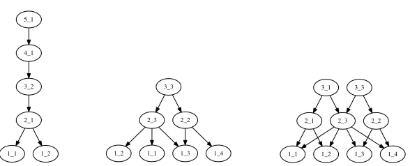
Figure 2: Extracted from the network shown in Figure 1, the left plot is a tree rooted at node 5 1,
the middle plot is a tree rooted at node 3 3, and the right plot is a subnetwork consisting of both the tree rooted at node 3 1 and the tree rooted at node 3 3.
Thus for visualization, it is straightforward to project the Kt topics/hidden units/factor
loadings/nodes of layer t ∈ {1, . . . , T} to the bottom data layer as the columns of the
V ×Kt matrix
t
Y
`=1
Φ(`), (13)
and rank their popularities using theKt dimensional nonnegative weight vector
r(t):=
" T
Y
`=t+1 Φ(`)
#
r. (14)
To measure the connection strength between node k of layer t and node k0 of layer t−1,
we use the value of
Φ(t)(k0, k),
which is also expressed as φ(kt)(k0) or φ(kt0)k.
Our intuition is that examining the nodes of the hidden layers, via their projections to the bottom data layer, from the top to bottom layers will gradually reveal less general and more specific aspects of the data. To verify this intuition and further understand the relationships between the general and specific aspects of the data, we consider extracting
a tree for each node of layer t, where t ≥2, to help visualize the inferred multilayer deep
structure. To be more specific, to construct a tree rooted at a node of layer t, we grow the
tree downward by linking the root node (if at layer t) or each leaf node of the tree (if at a
layer below layert) to all the nodes at the layer below that are connected to the root/leaf
2.3.1 Visualizing Nodes of Different Layers
Before presenting the technical details, we first provide some example results obtained with the PGBN on extracting multilayer representations from the 11,269 training documents
of the 20newsgroups data set (http://qwone.com/∼jason/20Newsgroups/). Given a fixed
budget ofK1 max = 800 on the width of the first layer, withη(t) = 0.1 for all t, a five-layer
deep network inferred by the PGBN has a network structure as [K1, K2, K3, K4, K5] =
[386,63,58,54,51], meaning that there are 386, 63, 58, 54, and 51 nodes at layers one to
five, respectively.
For visualization, we first relabel the nodes at each layer based on their weights{rk(t)}1,Kt,
calculated as in (14), with a more popular (larger weight) node assigned with a smaller label.
We visualize node k of layer t by displaying its top 12 words ranked according to their
probabilities in Qt−1
`=1Φ (`)
φ(kt), thekth column of the projected representation calculated
as in (13). We set the font size of node k of layer t proportional to r(kt)/r1(t)
1
10 in each
subplot, and color the outside border of a text box as red, green, orange, blue, or black for a node of layer five, four, three, two, or one, respectively. For better interpretation, we also exclude from the vocabulary the top 30 words of node 1 of layer one: “don just like people think know time good make way does writes edu ve want say really article use right did things point going better thing need sure used little,” and the top 20 words of node 2 of layer one: “edu writes article com apr cs ca just know don like think news cc david university john org wrote world.” These 50 words are not in the standard list of stopwords but can be considered as stopwords specific to the 20newsgroups corpus discovered by the PGBN.
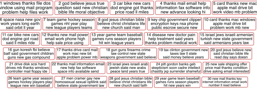
For the [386,63,58,54,51] PGBN learned on the 20newsgroups corpus, we plot 54
ex-ample topics of layer one in Figure 3, the top 30 topics of layer three in Figure 4, and the top 30 topics of layer five in Figure 5. Figure 3 clearly shows that the topics of layer one, except for topics 1-3 that mainly consist of common functional words of the corpus, are all very specific. For example, topics 71 and 81 shown in the first row are about “candida yeast symptoms” and “sex,” respectively, topics 53, 73, 83, and 84 shown in the second row are about “printer,” “msg,” “police radar detector,” and “Canadian health care sys-tem,” respectively, and topics 46 and 76 shown in third row are about “ice hockey” and “second amendment,” respectively. By contrast, the topics of layers three and five, shown in Figures 4 and 5, respectively, are much less specific and can in general be matched
to one or two news groups out of the 20 news groups, including comp.{graphics,
os.ms-windows.misc, sys.ibm.pc.hardware, sys.mac.hardware, windows.x}, rec.{autos,
motorcy-cles}, rec.sport.{baseball, hockey}, sci.{crypt, electronics, med, space}, misc.forsale, talk.
politics.{misc, guns, mideast}, and{talk.religion.misc, alt.atheism, soc.religion.christian}.
2.3.2 Visualizing Trees Rooted at The Top-Layer Hidden Units
While it is interesting to examine the topics of different layers to understand the general and specific aspects of the corpus used to train the PGBN, it would be more informative to further illustrate how the topics of different layers are related to each other. Thus we consider constructing trees to visualize the PGBN. We first pick a node as the root of a tree
and grow the tree downward by drawing a line from node k at layer t, the root or a leaf
1 doesn new problem work probably let said years ll long question course 11 team game hockey season games nhl year league teams players play cup 21 disease doctor pain treatment medical patients medicine cancer help skin blood problems 31 key chip bit keys number serial encrypted bits clipper escrow algorithm des 41 henry toronto zoo spencer work utzoo zoology man umd kipling eng allen 51 ground wire wiring neutral outlets circuit cable electrical wires outlet connected house 61 callison uoknor james car ecn lights uokmax fake bird continental alarm slb 71 candida yeast noring steve symptoms jon vitamin dyer body quack patients sinus 81 sex child copy women children protection pregnancy depression abstinence sexual education sehari 2 michael netcom andrew new uucp internet mark steve opinions mike mail net 12 sale new shipping offer condition price asking sell cover cd interested best 22 space nasa earth orbit gov data shuttle mission lunar spacecraft solar jpl 32 israel israeli lebanese lebanon attacks peace arab israelis civilians killed palestinian soldiers 42 graphics ftp pub data ray risc contact sgi machines pc instruction mail 52 won lost san new kaldis rutgers york houston st astros louis reds 62 sweden fi finland germany canada players finnish german april swedish wc czech 72 gatech prism gt georgia atlanta technology institute internet uucp gilkey hydra lankford 82 hall dave fame smith eddie murray winfield kingman yount steve guys bsu 3 thanks mail email help fax advance looking hi info information phone send 13 power output input high signal low voltage chip radio battery circuit data 23 gun guns firearms crime control weapons self criminals defense handgun firearm violent 33 cramer men gay homosexual optilink sexual clayton sex homosexuals homosexuality male virginia 43 ohio state magnus acs drugs ncr atlantaga wilson ncratl legal war ryan 53 printer hp print laser ink printers deskjet postscript bj canon quality toner 63 rit isc ultb bobby mozumder snm religious religion eric mom atheist men 73 msg dyer spdcc glutamate food effects brain studies humans blood olney foods 83 radar detector detectors police car beam illegal antenna radio virginia law band 4 god jesus christian bible christ christians life faith believe man christianity church 14 law government rights state court laws states public case civil legal federal 24 koresh fbi batf gas stratus compound waco children atf cdt believe government 34 turkish armenian armenians turks armenia turkey genocide soviet today russian government war 44 dod bmw ride motorcycle shaft rider motorcycles rec denizens club level list 54 ted colorado frank thf kimbark teel uchicago khan psu large psuvm cso 64 sandvik kent apple newton private alink ksand activities net cheers order royalroads 74 lib libxmu xmu ld symbol undefined doug usr imake problem sunos error 84 insurance health private care canada coverage canadian hospital medical pay public national 5 mac apple mhz modem ram bit card speed port board simms memory 15 bike dod ride bikes riding motorcycle sun left road bnr ama honda 25 jews israel israeli jewish arab arabs land center policy anti research palestine 35 pitt gordon banks geb skepticism cadre chastity intellect jxp soon surrender shameful 45 uiuc cso uxa ux illinois urbana josh manta cka hopkins champaign amin 55 uga georgia michael ai covington mcovingt easter programs jayne athens amateur research 65 speed car drive manual drivers traffic cars fuel automatic auto lane shift 75 behanna nec nj lock syl chris dod cb pack bike ll wide 85 war iran jury farid energy bombing hussein iraq military iraqi bomb civilians 6 available software version ftp server file sun program unix mit information code 16 clipper government chip key encryption nsa phone crypto secure keys netcom public 26 said went didn came told saw home left started says took apartment 36 scsi mb bus ide controller isa bit pc drive data mac os 46 period play power pp puck goal flyers shots pts scorer second lindros 56 problem polygon algorithm points reference edge cartridge program surface curve line edges 66 fred software ti mccall dseg nick level process mksol negev bedouin safety 76 militia amendment arms bear second constitution regulated government shall state ulowell organized 86 font fonts tt truetype type atm printer characters adobe ps character print
Figure 3: Example topics of layer one of the PGBN trained on the 20newsgroups corpus.
1 thanks mail email information help fax software info advance looking new hi
2 mac apple thanks bit mhz card modem ram speed port board memory
3 god jesus believe christian bible true question life christians said faith christ
4 car cars new engine miles dealer price drive
year road buy speed
5 windows dos file files thanks problem program using
run running win ms 6 team game hockey season
games nhl year play league new players teams
7 year game team baseball runs games season players
hit win league years
8 god jesus christian bible christ believe christians church
life faith man said
9 bike dod ride bikes riding motorcycle got sun
left new said ll
10 window thanks widget application using display available program
mail server set software 11 power thanks mail output
input high work line using low phone circuit
12 government key encryption clipper chip nsa phone public keys secure crypto escrow
13 gun guns firearms crime control law weapons state new self government said
14 disease doctor pain new help treatment medical years said problem thanks patients
15 card monitor video vga windows thanks drivers cards
mode mail graphics ati 16 drive scsi disk hard
drives mb windows thanks controller floppy mail ide
17 space nasa new gov work henry long doesn
said believe let ll
18 israel jews israeli arab jewish state arabs peace land policy new years
19 new sale shipping offer price mail condition drive thanks asking email interested
20 space nasa new information gov earth data orbit research program shuttle national
21 koresh fbi batf believe gas compound children stratus
waco said atf government
22 new sale shipping thanks mail offer price condition email interested asking best
23 new uiuc believe said cso read let ll doesn says long post
24 objective morality moral keith frank values livesey jon
wrong caltech sgi isn
25 tax clinton taxes government new money ll house pay look bush congress 26 law new state government
said president mr rights states information public national
27 men cramer gay homosexual sexual optilink clayton sex homosexuals homosexuality male state
28 space nasa new work gov henry long doesn
ll said believe let
29 pitt gordon banks geb skepticism soon cadre intellect chastity jxp surrender shameful
30 turkish armenian armenians turks armenia turkey government genocide
soviet said today new
Figure 4: The top 30 topics of layer three of the PGBN trained on the 20newsgroups corpus.
1 windows thanks file dos window using mail program
problem help files work
2 god believe jesus true question said new christian
bible life moral objective
3 car bike new cars dod engine got thanks
price road ll miles
4 thanks mail email help information fax software info
new advance looking hi
5 card thanks new mac apple mail drive bit work video mb problem
6 space nasa new gov work years long earth
said orbit ll year
7 team game hockey season games nhl year play new league players teams
8 god jesus christian bible believe christ christians life new church said man
9 key chip government clipper encryption keys nsa phone
public escrow secure new
10 card thanks mac windows apple mail drive bit problem work mb new
11 car bike new cars dod engine got road said ll miles ride
12 thanks new mail power email work phone high
help sale price using
13 year game team baseball games runs season players
hit win league years
14 disease new doctor pain help treatment said years thanks problem medical work
15 israel jews israeli armenian turkish new state government said armenians years law
16 gun koresh fbi believe batf said government children
guns new gas compound
17 thanks drive card mail work mac new bit apple problem power mb
18 gun guns firearms crime law control new state weapons government said believe
19 tax clinton government new taxes law ll state said money believe years
20 god jesus believe new said christian bible life
read day says doesn
21 drive disk scsi hard drives mb thanks windows
controller mail floppy ide
22 thanks mail information email new help fax software space info available send
23 israel jews israeli arab jewish state new arabs
peace land years true
24 pitt gordon banks geb skepticism soon cadre intellect chastity jxp surrender shameful
25 new sale shipping offer price mail thanks condition drive asking email interested
26 team game year season games hockey players play league new win baseball
27 men cramer gay new homosexual sexual optilink said
believe state government law
28 god jesus christian bible believe christ christians life new church said faith
29 year game team baseball games runs season players
hit new years win
30 new mail thanks key internet information email work
number ll read believe
1 windows thanks file dos window using mail program problem help files work
1 windows thanks file dos window using mail program problem help files work
1 thanks mail email information help fax software info advance looking new hi 5 windows dos file files
thanks problem program using run running win ms
10 window thanks widget application using display available program
mail server set software 15 card monitor video vga
windows thanks drivers cards mode mail graphics ati
1 thanks mail email information help fax software info advance new looking send 26 image jpeg gif file
files color images bit format thanks windows program
6 windows dos file problem thanks files using program
run win running ms
9 window thanks widget application using display available program
mail server set software 16 card monitor video vga
windows drivers thanks cards mode mail graphics ati
1 doesn new problem work probably let said years ll long question course 2 michael netcom andrew new uucp internet mark steve opinions mike mail net 3 thanks mail email help fax advance looking hi info information phone send 6 available software version ftp server file sun program unix mit information code 7 new information national research program year april center washington general years dr 42 graphics ftp pub data ray risc contact sgi machines pc instruction mail 56 problem polygon algorithm points reference edge cartridge program surface curve line edges 59 au australia oz mark philips canberra melbourne qdeck uwa quarterdeck network prl 69 graphics group ch comp umich split aspects groups engin radiosity grafsys hidden 8 windows dos file files problem program run using win disk ms driver 27 image jpeg gif color files file images format bit display graphics program 39 uk ac ed picture dcs sleeve liverpool demon tony simon oxford warwick 53 printer hp print laser ink printers deskjet postscript bj canon quality toner 86 font fonts tt truetype type atm printer characters adobe ps character print 18 window widget application display manager set using problem visual color value xlib 68 xterm keyboard key echo keys title host set keycode sequences ff hostname 74 lib libxmu xmu ld symbol undefined doug usr imake problem sunos error 17 card monitor video vga drivers cards mode ati graphics screen svga driver
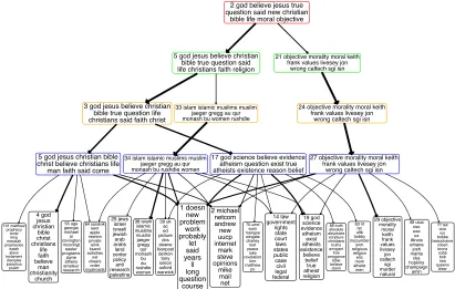
Figure 6: A [18,5,4,1,1] tree that includes all the lower-layer nodes (directly or indirectly) linked
with non-negligible weights to the top ranked node of the top layer, taken from the full [386,63,58,54,51] network inferred by the PGBN on the 11,269 training documents of the 20newsgroups corpus, withη(t)= 0.1 for allt. A line from nodekat layertto nodek0
at layert−1 indicates thatΦ(t)(k0, k)>3/Kt−1, with the width of the line proportional
to
q
Φ(t)(k0, k). For each node, the rank (in terms of popularity) at the corresponding
layer and the top 12 words of the corresponding topic are displayed inside the text box, where the text font size monotonically decreases as the popularity of the node decreases, and the outside border of the text box is colored as red, green, orange, blue, or black if the node is at layer five, four, three, two, or one, respectively.
where we set the width of the line connecting node k of layer t to node k0 of layer t−1
be proportional to q
Φ(t)(k0, k) and use τ
t to adjust the complexity of a tree. In general,
increasing τt would discard more weak connections and hence make the tree simpler and
easier to visualize.
We set τt= 3 for all tto visualize both a five-layer tree rooted at the top ranked node
2 god believe jesus true question said new christian
bible life moral objective
5 god jesus believe christian bible true question said life christians faith religion
21 objective morality moral keith frank values livesey jon
wrong caltech sgi isn
3 god jesus believe christian bible true question life christians said faith christ
33 islam islamic muslims muslim jaeger gregg au qur monash bu women rushdie
24 objective morality moral keith frank values livesey jon
wrong caltech sgi isn
5 god jesus christian bible christ believe christians life man faith said come
17 god science believe evidence atheism question exist true atheists existence reason belief 34 islam islamic muslims muslim
jaeger gregg au qur monash bu rushdie women
1 doesn new problem work probably let said years ll long question course 2 michael netcom andrew new uucp internet mark steve opinions mike mail net 4 god jesus christian bible christ christians life faith believe man christianity church 55 uga georgia michael ai covington mcovingt easter programs jayne athens amateur research 64 sandvik kent apple newton private alink ksand activities net cheers order royalroads 101 matthew prophecy tomb king messiah prophecies isaiah jesus testament disciples josephus psalm 14 law government rights state court laws states public case civil legal federal 19 god science evidence atheism exist atheists existence believe belief true atheist religion 39 uk ac ed picture dcs sleeve liverpool demon tony simon oxford warwick 63 rit isc ultb bobby mozumder snm religious religion eric mom atheist men 70 umd wam mangoe wingate charley text peace luke revelation kmr matthew po 88 truth absolute absolutes scripture christians truths arrogant true arrogance bible believe claim 25 jews israel israeli jewish arab arabs land center policy anti research palestine 38 islam islamic muslims muslim jaeger gregg qur monash bu au rushdie women
27 objective morality moral keith frank values livesey jon
wrong caltech sgi isn
29 objective morality moral keith frank values livesey jon caltech sgi murder natural 45 uiuc cso uxa ux illinois urbana josh manta cka hopkins champaign amin 77 tek vice ico bobbe beauchaine robert bronx cobb bob sea queens blew
Figure 7: Analogous plot to Figure 6 for a tree on “religion,” rooted at node 2 of the top-layer.
Following the branches of each tree shown in both figures, it is clear that the topics become more and more specific when moving along the tree from the top to bottom. Taking the tree on “religion” shown in Figure 7 for example, the root node splits into two nodes when moving from layers five to four: while the left node is still mainly about “religion,” the right node is on “objective morality.” When moving from layers four to three, node 5 of layer four splits into a node about “Christian” and another node about “Islamic.” When moving from layers three to two, node 3 of layer three splits into a node about “God, Jesus, & Christian,” and another node about “science, atheism, & question of the existence of God.” When moving from layers two to one, all four nodes of layer two split into multiple topics, and they are all strongly connected to both topics 1 and 2 of layer one, whose top words are those that appear frequently in the 20newsgroups corpus.
2.3.3 Visualizing Subnetworks Consisting of Related Trees
Examining the top-layer topics shown in Figure 5, one may find that some of the nodes seem to be closely related to each other. For example, topics 3 and 11 share eleven words out of the top twelve ones; topics 15 and 23 both have “Israel” and “Jews” as their top two words; topics 16 and 18 are both related to “gun;” and topics 7, 13, and 26 all share “team(s),” “game(s),” “player(s),” “season,” and “league.”
that topic 15 differs from topic 23 in that it is not only about “Israel & Arabs,” but also about “Israel, Armenia, & Turkey.” It is clear from Figure 19 in that topic 16 differs from topic 18 in that it is mainly about Waco siege happened in 1993 involving David Koresh, the Federal Bureau of Investigation (FBI), and the Bureau of Alcohol, Tobacco, Firearms and Explosives (BATF). It is clear from Figure 20 that topics 7 and 13 are mainly about “ice hockey” and “baseball,” respectively, and topic 26 is a mixture of both.
2.3.4 Capturing Correlations Between Nodes
For the augmentable GBN, as in (18), given the weight vectorθ(1)j , we have
Ex(1)j Φ(1),θ
(1)
j
=Φ(1)θ(1)j . (15)
A distinction between a shallow augmentable GBN with T = 1 hidden layer and a deep
augmentable GBN with T ≥2 hidden layers is that the prior forθ(1)j changes from θ(1)j ∼
Gam(r,1/c(2)j ) for T = 1 to θ(1)j ∼ Gam(Φ(2)θ(2)j ,1/c(2)j ) for T ≥ 2. For the GBN with
T = 1, given the shared weight vector r, we have
Ex(1)j
Φ(1),r
=Φ(1)r/c(2)j ; (16)
for the GBN with T = 2, given the shared weight vectorr, we have
Ex(1)j
Φ(1),Φ(2),r
=Φ(1)Φ(2)r. c(2)j c(3)j ; (17)
and for the GBN withT ≥2, given the weight vectorθ(2)j , we have
Ex(1)j
Φ(1),Φ(2),θ
(2)
j
=Φ(1)Φ(2)θ(2)j /c(2)j . (18)
Thus in the prior, the co-occurrence patterns of the columns ofΦ(1) are modeled by only a
single vectorrwhenT = 1, but are captured in the columns ofΦ(2)whenT ≥2. Similarly,
in the prior, if T ≥ t+ 1, the co-occurrence patterns of the Kt columns of the projected
topicsQt
`=1Φ
(`) will be captured in the columns of theK
t×Kt+1 matrixΦ(t+1).
To be more specific, we show in Figure 21 in Appendix C three example trees rooted
at three different nodes of layer three, where we lower the threshold to τt = 1 to reveal
more weak links between the nodes of adjacent layers. The top subplot reveals that, in addition to strongly co-occurring with the top two topics of layer one, topic 21 of layer one on “medicine” tends to co-occur not only with topics 7, 21, and 26, which are all common topics that frequently appear, but also with some much less common topics that are related to very specific diseases or symptoms, such as topic 67 on “msg” and “Chinese restaurant syndrome,” topic 73 on “candida yeast symptoms,” and topic 180 on “acidophilous” and “astemizole (hismanal).”
The bottom subplot reveals that in layer one, topic 14 on “law & government,” topic 32 on “Israel & Lebanon,” topic 34 on “Turkey, Armenia, Soviet Union, & Russian,” topic 132 on “Greece, Turkey, & Cyprus,” topic 98 on “Bosnia, Serbs, & Muslims,” topic 143 on “Armenia, Azeris, Cyprus, Turkey, & Karabakh,” and several other very specific topics related to Turkey and/or Armenia all tend to co-occur with each other.
We note that capturing the co-occurrence patterns between the topics not only helps exploratory data analysis, but also helps extract better features for classification in an unsupervised manner and improves prediction for held-out data, as will be demonstrated in detail in Section 4.
2.4 Related Models
The structure of the augmentable GBN resembles the sigmoid belief network and recently proposed deep exponential family model (Ranganath et al., 2014b). Such kind of gamma distribution based network and its inference procedure were vaguely hinted in Corollary 2 of Zhou and Carin (2015), and had been exploited by Acharya et al. (2015) to develop a gamma Markov chain to model the temporal evolution of the factor scores of a dynamic count matrix, but have not yet been investigated for extracting multilayer data represen-tations. The proposed augmentable GBN may also be considered as an exponential family harmonium (Welling et al., 2004; Xing et al., 2005).
2.4.1 Sigmoid and Deep Belief Networks
Under the hierarchical model in (1), given the connection weight matrices, the joint distri-bution of the observed/latent counts and gamma hidden units of the GBN can be expressed, similar to those of the sigmoid and deep belief networks (Bengio et al., 2015), as
P
x(1)j ,{θ(jt)}t
{Φ
(t)}
t
=P
x(1)j
Φ
(1),θ(1)
j
"T−1
Y
t=1
P
θ(jt)
Φ
(t+1),θ(t+1)
j
#
P
θ(jT)
.
Withφv:representing the vth row Φ, for the gamma hidden unitsθvj(t) we have
P
θ(vjt)
φ
(t+1)
v: ,θ (t+1)
j , c
(t+1)
j+1
=
c(jt+1+1)
φ(vt:+1)θ (t+1)
j
Γ
φ(vt:+1)θ(jt+1)
θ(vjt)
φ(vt:+1)θ (t+1)
j −1
e−c
(t+1)
j+1 θ (t)
vj, (19)
which are highly nonlinear functions that are strongly desired in deep learning. By contrast,
with the sigmoid function σ(x) = 1/(1 +e−x) and bias terms b(vt+1), a sigmoid/deep belief
network would connect the binary hidden units θvj(t) ∈ {0,1} of layer t (for deep belief
networks,t < T −1 ) to the product of the connection weights and binary hidden units of
the next layer with
P
θ(vjt)= 1
φ
(t+1)
v: ,θ (t+1)
j , b
(t+1)
v
=σ
bv(t+1)+φv(t:+1)θ(jt+1)
. (20)
limitation of binary units in capturing the approximately linear data structure over small ranges is a key motivation for Frey and Hinton (1999) to investigate nonlinear Gaussian belief networks with real-valued units. As a new alternative to binary units, it would be interesting to further investigate whether the gamma distributed nonnegative real units can in theory carry richer information and model more complex nonlinearities given the same network structure. Note that the rectified linear units have emerged as powerful alternatives of sigmoid units to introduce nonlinearity (Nair and Hinton, 2010). It would be interesting to investigate whether the gamma units can be used to introduce nonlinearity into the positive region of the rectified linear units.
2.4.2 Deep Poisson Factor Analysis
WithT = 1, the PGBN specified by (1)-(3) and (8) reduces to Poisson factor analysis (PFA)
using the (truncated) gamma-negative binomial process (Zhou and Carin, 2015), with a
truncation level of K1. As discussed in (Zhou et al., 2012; Zhou and Carin, 2015), with
priors imposed on neitherφ(1)k norθ(1)j , PFA is related to nonnegative matrix factorization
(Lee and Seung, 2001), and with the Dirichlet priors imposed on both φ(1)k and θ(1)j , PFA
is related to latent Dirichlet allocation (Blei et al., 2003).
Related to the PGBN and the dynamic model in (Acharya et al., 2015), the deep ex-ponential family model of Ranganath et al. (2014b) also considers a gamma chain under Poisson observations, but it is the gamma scale parameters that are chained and factorized, which allows learning the network parameters using black box variational inference (Ran-ganath et al., 2014a). In the proposed PGBN, we chain the gamma random variables via the gamma shape parameters. Both strategies worth through investigation. We prefer chain-ing the shape parameters in this paper, which leads to efficient upward-downward Gibbs sampling via data augmentation and makes it clear how the latent counts are propagated across layers, as discussed in detail in the following sections. The sigmoid belief network has also been recently incorporated into PFA for deep factorization of count data (Gan et al., 2015a), however, that deep structure captures only the correlations between binary factor usage patterns but not the full connection weights. In addition, neither Ranganath et al. (2014b) nor Gan et al. (2015a) provide a principled way to learn the network struc-ture, whereas the proposed GBN uses the gamma-negative binomial process together with a greedy layer-wise training strategy to automatically infer the widths of the hidden layers, which will be described in Section 3.3.
2.4.3 Correlated and Tree-Structured Topic Models
The PGBN with T = 2 can also be related to correlated topic models (Blei and Lafferty,
2006; Paisley et al., 2012; Chen et al., 2013; Ranganath and Blei, 2015; Linderman et al., 2015), which typically use the logistic normal distributions to replace the topic-proportion Dirichlet distributions used in latent Dirichlet allocation (Blei et al., 2003), capturing the co-occurrence patterns between the topics in the latent Gaussian space using a covariance matrix. By contrast, the PGBN factorizes the topic usage weights (not proportions) under the gamma likelihood, capturing the co-occurrence patterns between the topics of the first
layer (i.e., the columns ofΦ(1)) in the columns ofΦ(2), the latent weight matrix connecting
matrix inversion, which is often necessary for correlated topic models without specially structured covariance matrices, and scales linearly with the number of topics, hence it is suitable to be used to capture the correlations between hundreds of or thousands of topics. As in Figures 6, 7, and 17-21, trees and subnetworks can be extracted from the inferred deep network to visualize the data. Tree-structured topic models have also been proposed before, such as those in Blei et al. (2010), Adams et al. (2010), and Paisley et al. (2015), but they usually artificially impose the tree structures to be learned, whereas the PGBN learns a directed network, from which trees and subnetworks can be extracted for visualization, without the need to specify the number of nodes per layer, restrict the number of branches per node, and forbid a node to have multiple parents.
3. Model Properties and Inference
Inference for the GBN shown in (1) appears challenging, because not only the conjugate prior is unknown for the shape parameter of a gamma distribution, but also the gradients are difficult to evaluate for the parameters of the (log) gamma probability density function, which, as in (19), includes the parameters inside the (log) gamma function. To address these challenges, we consider data augmentation (van Dyk and Meng, 2001) that intro-duces auxiliary variables to make it simple to compute the conditional posteriors of model parameters via the joint distribution of the auxiliary and existing random variables. We will first show that each gamma hidden unit can be linked to a Poisson distributed latent count variable, leading to a negative binomial likelihood for the parameters of the gamma hidden unit if it is margined out from the Poisson distribution; we then introduce an auxiliary count variable, which is sampled from the CRT distribution parametrized by the negative binomial latent count and shape parameter, to make the joint likelihood of the auxiliary CRT count and latent negative binomial count given the parameters of the gamma hidden unit amenable to posterior simulation. More specifically, under the proposed augmentation scheme, the gamma shape parameters will be linked to auxiliary counts under the Poisson likelihoods, making it straightforward for posterior simulation, as described below in detail.
3.1 The Upward Propagation of Latent Counts
We break the inference of the GBN ofT hidden layers into T related subproblems, each of
which is solved with the same subroutine. Thus for implementation, it is straightforward
for the GBN to adjust its depth T. Let us denote x(jt) ∈ ZKt−1 as the observed or latent
count vector of layert∈ {1, . . . , T}, and xvj(t) as its vth element, where v∈ {1, . . . , Kt−1}.
Lemma 1 (Augment-and-Conquer The Gamma Belief Network) Withp(1)j := 1−
e−1 and
p(jt+1):=−ln(1−p(jt)) . h
c(jt+1)−ln(1−p(jt)) i
(21)
for t= 1, . . . , T, one may connect the observed or latent counts x(jt) ∈ZKt−1 to the product
Φ(t)θ(jt) at layert under the Poisson likelihood as
x(jt) ∼Pois h
−Φ(t)θ(jt)ln
1−p(jt) i
Proof By definition (22) is true for layer t = 1. Suppose that (22) is also true for layer
t >1, then we can augment each count x(vjt), where v∈ {1, . . . , Kt−1}, into the summation
of Ktlatent counts, which are smaller than or equal to x(vjt) as
x(vjt)=
Kt
X
k=1
x(vjkt) , x(vjkt) ∼Pois h
−φ(vkt)θkj(t)ln
1−p(jt) i
. (23)
Let the· symbol represent summing over the corresponding index and let
m(kjt)(t+1) :=x(·jkt) :=
Kt−1 X
v=1
x(vjkt)
represent the number of times that factork∈ {1, . . . , Kt}of layertappears in observationj
andm(jt)(t+1) :=x·(jt)1, . . . , x(·jKt)
t
0
. SincePKt−1
v=1 φ (t)
vk = 1, we can marginalize outΦ
(t) as in
(Zhou et al., 2012), leading to
mj(t)(t+1)∼Poish−θj(t)ln1−p(jt)i.
Further marginalizing out the gamma distributedθ(jt) from the Poisson likelihood leads to
m(jt)(t+1) ∼NB
Φ(t+1)θ(jt+1), p(jt+1)
. (24)
Elementk ofm(jt)(t+1) can be augmented under its compound Poisson representation as
m(kjt)(t+1)=
x(kjt+1)
X
`=1
u`, u`∼Log(p
(t+1)
j ), x
(t+1)
kj ∼Pois
h
−φ(kt:+1)θ(jt+1)ln
1−p(jt+1)
i .
Thus if (22) is true for layer t, then it is also true for layert+ 1.
Corollary 2 (Propagate the latent counts upward) Using Lemma 4.1 of (Zhou et al., 2012) on (23) and Theorem 1 of (Zhou and Carin, 2015) on (24), we can propagate the
latent counts x(vjt) of layer t upward to layer t+ 1 as
n
x(vjt)1, . . . , x(vjKt)
t
x
(t)
vj,φ
(t)
v:,θ (t)
j
o
∼Mult
x
(t)
vj,
φ(vt1)θ(1tj)
PKt
k=1φ (t)
vkθ
(t)
kj
, . . . , φ
(t)
vKtθ (t)
Ktj
PKt
k=1φ (t)
vkθ
(t)
kj
,(25)
x(kjt+1)
m
(t)(t+1)
kj ,φ
(t+1)
k: ,θ (t+1)
j
( )1 j x
( )1
( )1 j
θ ( )2
( )2 j
θ ( )3
( )3
j c
( )T j
θ (T+1)
j
c r 0
c0
J
( )1 j
p
( )2 j
c
(a)
( )1 j
x ( )1
( )1 j θ J ( ) { } 1 vjk
x ( )1 j
p ( )2
( )2 j
θ ( )3
( )3
j c
( )2 j
c
(b)
( )1 j
x ( )1
( )1 j θ J ( ) { } 1 vjk x
( )2
( )2 j
θ ( )3
( )3
j c ( )( ) { } 1 2 kj m
( )2 j c
( )1 j
p
(c)
( )1 j
x ( )1
J ( ) { } 1 vjk x
( )2 j
p ( )2
( )2 j
θ ( )3
( )3
j c ( )( ) { } 1 2 kj m (d)
( )1 j
x ( )1
J ( ) { } 1 vjk x
( )2 j
p ( )2
( )2 j
θ
( )3
( )3 j c ( )( ) { } 1 2 kj m
( )2 j
x
(e)
( )1 j
x
( )1 J ( ) { } 1 vjk x
( )2 j
θ ( )3
( )3
j c ( )( ) { } 1 2 kj m
( )2 j
x ( )2
j
p ( )2
(f)
J
( )t j x ( ) { } t vjk x
( )t
( )( ) { } t t+1 kj m
(t+1) j
x
(t+1)
(t+1)
j
θ
(t+1)
j
p (t+2)
(t+2)
j
c
(g)
J
( )T j x ( ) { } T vjk x ( )T
( )( ) { } T T+1 kj m
(T+1) j
x (T+1) j p
r
0
c0
(h)
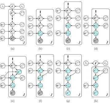
Figure 8: Graphical representations of the model and data augmentation and marginalization based
inference scheme. (a) graphical representation of the GBN hierarchical model. (b) an augmented representation of Poisson factor model of layert= 1, corresponding to (23) witht= 1. (c) an alternative representation using the relationships between the Poisson and multinomial distributions, obtained by applying Lemma 4.1 of (Zhou et al., 2012) on (23) fort= 1. (d) a negative binomial distribution based representation that marginal-izes out the gamma from the Poisson distributions, corresponding to (24) fort= 1. (e) an equivalent representation that introduces CRT distributed auxiliary variables, corre-sponding to (26) witht= 1. (f) an equivalent representation using Theorem 1 of (Zhou and Carin, 2015) on (24) and (26) fort= 1. (g) An representation obtained by repeating the same augmentation-marginalization steps described in (b)-(f) one layer at a time from layers 1 tot. (h) An representation of the top hidden layer.
Note thatx(·jt) =m(·jt)(t+1), and as the number of tables occupied by the customers is in
the same order as the logarithm of the customer number in a Chinese restaurant process,
xkj(t+1) is in the same order as ln mkj(t)(t+1). Thus the total count of layert+ 1 as P
jx
(t+1)
·j
would often be much smaller than that of layer tasP
jx
(t)
·j (though in general not as small
as a count that is in the same order of the logarithm of P
jx
(t)
·j ), and hence one may use
the total countP
jx
(T)
layers to the GBN. In addition, if the latent countx(kt0)·k:=
P
jx
(t)
k0jk becomes close or equal
to zero, then the posterior mean of Φ(t)(k0, k) could become so small that node k0 of layer
t−1 can be considered to be disconnected from nodekof layer t.
3.2 Modeling Data Variability With Distributed Representation
In comparison to a single-layer model with T = 1, which assumes that the hidden units
of layer one are independent in the prior, the multilayer model with T ≥ 2 captures the
correlations between them. Note that for the extreme case that Φ(t) = IKt for t ≥ 2 are
all identity matrices, which indicates that there are no correlations between the features
of θ(jt−1) left to be captured, the deep structure could still provide benefits as it helps
model latent countsm(1)(2)j that may be highly overdispersed. For example, let us assume
Φ(t)=IK2 for all t≥2, then from (1) and (24) we have
m(1)(2)kj ∼NB(θ(2)kj, p(2)j ), . . . , θ(kjt)∼Gam(θ(kjt+1),1/c(jt+1)), . . . , θ(kjT) ∼Gam(rk,1/c(jT+1)).
Using the laws of total expectation and total variance, we have
Eθkj(2)|rk
= rk
QT+1
t=3 c (t)
j
, var
θkj(2)|rk
=rk
T+1
X
t=3
" t Y
`=3
c(j`)
−2# "TY+1
`=t+1
c(j`)
−1#
.
Further applying the same laws, we have
Em(1)(2)kj |rk
= rkp
(2)
j
1−p(2)j
QT+1
t=3 c (t)
j
,
varm(1)(2)kj |rk
= rkp
(2)
j
1−p(2)j 2QT+1
t=3 c (t)
j
(
1 +p(2)j
T+1
X
t=3
" t Y
`=3
c(j`)
−1
#)
.
Thus the variance-to-mean ratio (VMR) of the count m(1)(2)kj given rk can be expressed as
VMRm(1)(2)kj |rk
= 1
1−p(2)j
(
1 +p(2)j
T+1
X
t=3
" t Y
`=3
c(j`)
−1
#)
. (27)
In comparison to PFA withm(1)(2)kj ∼NB(rk, p
(2)
j ) givenrk, with a VMR of 1/(1−p
(2)
j ),
the GBN with T hidden layers, which mixes the shape of m(1)(2)kj ∼ NB(θ(2)kj, p(2)j ) with a
chain of gamma random variables, increases VMR
m(1)(2)kj |rk
by a factor of
1 +p(2)j
T+1
X
t=3
" t Y
`=3
c(j`)−1
#
,
which is equal to
1 + (T −1)p(2)j
if we further assumec(jt)= 1 for allt≥3. Therefore, by increasing the depth of the network
3.3 Learning The Network Structure With Layer-Wise Training
As jointly training all layers together is often difficult, existing deep networks are typically trained using a greedy layer-wise unsupervised training algorithm, such as the one proposed in (Hinton et al., 2006) to train the deep belief networks. The effectiveness of this training strategy is further analyzed in (Bengio et al., 2007). By contrast, the augmentable GBN has a simple Gibbs sampler to jointly train all its hidden layers, as described in Appendix B, and hence does not necessarily require greedy layer-wise training, but the same as these commonly used deep learning algorithms, it still needs to specify the number of layers and the width of each layer.
In this paper, we adopt the idea of layer-wise training for the GBN, not because of the lack of an effective joint-training algorithm that trains all layers together in each iteration, but for the purpose of learning the width of each hidden layer in a greedy layer-wise manner, given a fixed budget on the width of the first layer. The basic idea is to first train a
GBN with a single hidden layer, i.e., T = 1, for which we know how to use the
gamma-negative binomial process (Zhou and Carin, 2015; Zhou et al., 2015b) to infer the posterior
distribution of the number of active factors; we fix the width of the first layer K1 with the
number of active factors inferred at iterationB1, prune all inactive factors of the first layer,
and continue Gibbs sampling for another C1 iterations. Now we describe the proposed
recursive procedure to build a GBN withT ≥2 layers. With a GBN ofT−1 hidden layers
that has already been inferred, for which the hidden units of the top layer are distributed
as θ(jT−1) ∼ Gam(r,1/cj(T)), where r = (r1, . . . , rKT−1)
0, we add another layer by letting
θj(T−1) ∼ Gam(Φ(T)θ(jT),1/c(jT)), θj(T) ∼ Gam(r,1/c(jT+1)), where Φ(T) ∈ RKT−1×KTmax
+
and r is redefined as r = (r1, . . . , rKTmax)
0. The key idea is with latent counts m(T)(T+1)
kj
upward propagated from the bottom data layer, one may marginalize out θ(kjT), leading to
m(kjT)(T+1) ∼NB(rk, pj(T+1)), rk ∼ Gam(γ0/KTmax,1/c0), and hence can again rely on the
shrinkage mechanism of a truncated gamma-negative binomial process to prune inactive
factors (connection weight vectors, columns of Φ(T)) of layer T, making KT, the inferred
layer width for the newly added layer, smaller thanKTmaxifKTmaxis set to be sufficiently
large. The newly added layer and all the layers below would be jointly trained, but with the
structure below the newly added layer kept unchanged. Note that when T = 1, the GBN
infers the number of active factors ifK1 maxis set large enough, otherwise, it still assigns the
factors with different weightsrk, but may not be able to prune any of them. The details of
the proposed layer-wise training strategies are summarized in Algorithm 1 for multivariate count data, and in Algorithm 2 for multivariate binary and nonnegative real data.
4. Experimental Results
In this section, we present experimental results for count, binary, and nonnegative real data.
4.1 Deep Topic Modeling
is identical to the (truncated) gamma-negative binomial process PFA of Zhou and Carin (2015), which is a nonparametric Bayesian algorithm that performs similarly to the hierar-chical Dirichlet process latent Dirichlet allocation of Teh et al. (2006) for text analysis, and is considered as a strong baseline. Thus we will focus on making comparison to the PGBN with a single layer, with its layer width set to be large to approximate the performance of the gamma-negative binomial process PFA. We evaluate the PGBNs’ performance by ex-amining both how well they unsupervisedly extract low-dimensional features for document classification, and how well they predict heldout word tokens. Matlab code will be available in http://mingyuanzhou.github.io/.
We use Algorithm 1 to learn, in a layer-wise manner, from the training data the
con-nection weight matrices Φ(1), . . . ,Φ(Tmax) and the top-layer hidden units’ gamma shape
parameters r: to add layer T to a previously trained network with T −1 layers, we use
BT iterations to jointly train Φ(T) and r together with {Φ(t)}1,T−1, prune the inactive
factors of layer T, and continue the joint training with another CT iterations. We set the
hyper-parameters as a0=b0= 0.01 and e0 =f0 = 1. Given the trained network, we apply
the upward-downward Gibbs sampler to collect 500 MCMC samples after 500 burnins to
estimate the posterior mean of the feature usage proportion vector θ(1)j /θ·(1)j at the first
hidden layer, for every document in both the training and testing sets.
4.1.1 Feature Learning for Binary Classification
We consider the 20newsgroups data set that consists of 18,774 documents from 20
dif-ferent news groups, with a vocabulary of size K0 = 61,188. It is partitioned into a
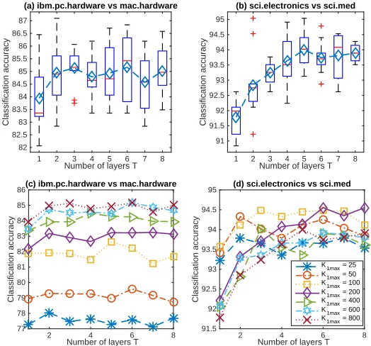
training set of 11,269 documents and a testing set of 7,505 ones. We first consider two
binary classification tasks that distinguish between the comp.sys.ibm.pc.hardware and
comp.sys.mac.hardware, and between the sci.electronics and sci.med news groups. For
each binary classification task, we remove a standard list of stop words and only consider the terms that appear at least five times, and report the classification accuracies based on 12 independent random trials. With the upper bound of the first layer’s width set as K1 max ∈ {25,50,100,200,400,600,800}, and Bt =Ct= 1000 and η(t) = 0.01 for all t, we
use Algorithm 1 to train a network withT ∈ {1,2, . . . ,8}layers. Denote ¯θj as the estimated
K1 dimensional feature vector for documentj, whereK1 ≤K1 max is the inferred number of
active factors of the first layer that is bounded by the pre-specified truncation levelK1 max.
We use the L2 regularized logistic regression provided by the LIBLINEAR package (Fan
et al., 2008) to train a linear classifier on ¯θj in the training set and use it to classify ¯θj in
the test set, where the regularization parameter is five-folder cross-validated on the training
set from (2−10,2−9, . . . ,215).
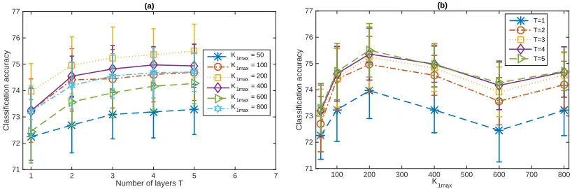
As shown in Figure 9, modifying the PGBN from a single-layer shallow network to a multilayer deep one clearly improves the qualities of the unsupervisedly extracted feature
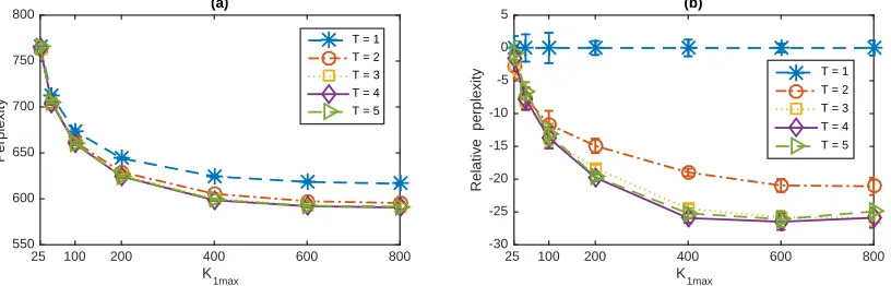
vectors. In a random trial, withK1 max= 800, we infer a network structure of [K1, . . . , K8] =
[512,154,75,54,47,37,34,29] for the first binary classification task, and [K1, . . . , K8] =
[491,143,74,49,36,32,28,26] for the second one. Figures 9(c)-(d) also show that increasing
![Figure 1: An example directed network of five hidden layers, with K0=8 visible units,[K1, K2, K3, K4, K5] = [6, 4, 3, 3, 2], and sparse connections between the units of adja-cent layers.](https://thumb-us.123doks.com/thumbv2/123dok_us/9797490.1965650/8.612.209.400.86.230/figure-example-directed-network-hidden-visible-sparse-connections.webp)
![Figure 6: A [18, 5, 4, 1, 1] tree that includes all the lower-layer nodes (directly or indirectly) linkedwith non-negligible weights to the top ranked node of the top layer, taken from the full[386, 63, 58, 54, 51] network inferred by the PGBN on the 11,26](https://thumb-us.123doks.com/thumbv2/123dok_us/9797490.1965650/12.612.102.516.77.299/includes-directly-indirectly-linkedwith-negligible-weights-network-inferred.webp)