A Novel Smart Grid State Estimation Method Based on Neural Networks

(1)

I. Introduction

T

HE smart grid technologies are a step towards developing the utility industry, whereas it could overcome the drawbacks of the existing power grid [1]. The high demand for electricity cannot serve the high increasing population rate and the low response. The manual control and the high losses during transmission made the manufacturers think about alternative solutions. Smart grids can deal with the needs of the high population [2], achieve reliability, automated control which leads to the high response, and decrease the losses in transmission lines by providing efficiency of data transmission from head to tail [3]–[5].

The feeding of the smart grid [6] can be renewable energy resources (e.g., photovoltaic (PV) and wind) in parallel with the utility grid to provide a low overall cost. On the other side, these resources have negative impacts on the distribution system, such as the high power loss due to the back feeding of the power flow [7], fluctuation and unbalanced voltage [8], and voltage rise [9].

Many researchers evaluated the steady-state conditions of distribution system by using the state-of-the-art techniques, such as Gauss-Seidel and Newton-Raphson, which supposed that the system is already stable [10]. The power flow techniques have been applied to determine the steady-state operation conditions during transmitting the electricity, Kirchhoff’s current law and other methods to determine the voltage magnitude, angle, and active/reactive power. Other iterative methods are detailed in [11], [12]. A technique for the multiphase unbalanced system, which was developed to deal with different types of loads (constant current, constant power, and constant impedance), is presented in [13]. To model the harmonics resulting by the variable load with the time variant, a simulator is modeled based on the openDSS program to estimate the value of harmonics [14].

Impact of PV integration was studied in [15]. A study for modeling and simulating the penetration effects by two feeders in different scenarios is illustrated in [16].

A quasi-static time-series (QSTS) is presented for analyzing and simulating the operation of PV distribution system and evaluating the effects of the PV integration during a specified duration (day or year).

In [17], several works have been proposed to reduce the execution time of QSTS. The authors presented two methods for shortening the time-series for power flow calculations in the presence of the distributed generation. The size of the input data, as well as the power flow calculation, was decreased. The first method depends on down-sampling data through reducing time resolution. This method has the disadvantage of losing the peak values during down-sampling. The second method chooses the similar intervals, and then performs the calculation on them. This method also has the disadvantage of missing the rest of data, which makes the simulations inaccurate.

In [18] and [19], the neural networks control the electrical systems with nonlinear dynamic characteristics. Ref [20] explained the use of neural networks with fully connected neuron learning combined with power flow for optimizing smart grids.

The limitation of the methods reported in the literature is that they take very long execution time to estimate smart grid state. In this paper, we propose a fast method (SE-NN) to calculate the state of the smart grid (voltage, active power, and reactive power) in a short time and accurate way using a neural network model.

II. Background

Power flow analysis is essential for monitoring system distribution by calculating active/reactive power, currents, and voltages at each time step for a specified duration. Iterative power flow methods are used for determining the operation of the system at the steady-state condition. In [21], a Newton-Raphson method algorithm was used for solving non-linear equations. The problem with this method is that the

Keywords

Neural Network, Smart Grid, Renewable Energy, Power Loss, Voltage Profile.

Abstract

The rapid development in smart grids needs efficient state estimation methods. This paper presents a novel method for smart grid state estimation (e.g., voltages, active and reactive power loss) using artificial neural networks (ANNs). The proposed method which is called SE-NN (state estimation using neural network) can evaluate the state at any point of smart grid systems considering fluctuated loads. To demonstrate the effectiveness of the proposed method, it has been applied on IEEE 33-bus distribution system with different data resolutions. The accuracy of the proposed method is validated by comparing the results with an exact power flow method. The proposed SE-NN method is a very fast tool to estimate voltages and re/active power loss with a high accuracy compared to the traditional methods.

A Novel Smart Grid State Estimation Method Based

on Neural Networks

Mohamed Abdel-Nasser*, Karar Mahmoud, Heba Kashef

Department of Electrical Engineering, Aswan University, 81542 Aswan (Egypt)

Received 27 December 2017 | Accepted 22 January 2018 | Published 29 January 2018

* Corresponding author.

E-mail address: [email protected]

(2)

memory space is not sufficient for large-scale systems. A modified Gauss-Seidel algorithm was presented in [22]. This algorithm solves the problem of the limited memory size with small execution time.

The state estimation is used for estimating the power flow solution of different real-time information because of the large number of nodes, few phase measurements, and disability of the system to be hardly provided with a meter at each node and each branch. The commonly used state estimator is weighted least square criteria (WLS). A study on state estimation depending on Tikhonov regularization compared with the WLS is detailed in [23]. Due to the changeable nature of the energy environment, the distribution system needs new system modeling that can adapt to the new advanced technologies. In [24], the authors discussed the new methodologies for wide area monitoring and analyzing of the smart grids. Another approach for wide-area network estimation called multi-area state estimation (MASE) is illustrated in [25]. This approach relies on a two-step procedure, the overall network area is divided into subareas according to its geographical characteristics and measurement estimator. The first step is performing all the available measurements for each area. The subareas have the same nodes number and the estimator is working in parallel for low execution time. In the second step, the data of the first step is processed and refined for different operation conditions. The previous methods have drawbacks of the long execution time [26]. In general, iterative power flow methods require a long time to estimate the states of the smart grid. In this paper, we propose a fast method for real-time analysis with high accuracy. To demonstrate the effectiveness of our method, we have compared it with a well-known power flow method.

III. The Proposed Method

A. Neural Networks

The artificial neural networks are a close simulation of the human brain. We use the neural network in state estimation because of its high efficiency in processing signals and predicting output in a fast and accurate way. The neural network model either contains one layer (input and output are directly connected), two layers (the first layer for receiving data, and the other layer for output results) or multilayer whereas three or more layers are connected in parallel (input layer, hidden layer(s), and output layer) [27]–[29].

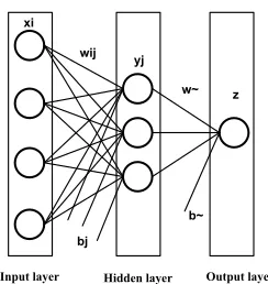
There are many algorithms to train neural networks; the preferable one is the back-propagation algorithm in which the error is calculated by computing the difference between the target and the measured output, and the weights are adjusted and propagated backward from the output to the input until finding the weights that minimize the error. Then the network is being learned for the desired output. More details about learning of neural network can be found in [30]. Fig. 1 shows a neural network containing three layers. The first layer is the input layer which contains four neurons, the second layer is the hidden layer that contains three neurons, and the last one is the output layer.

Input layer Hidden layer Output layer

wij

b~ w~

bj yj

z xi

Fig. 1. The architecture of neural networks.

The connection lines w and b denote the weights and biases. The output of the first layer can be expressed as follow:

∑

=

+

=

k

i i ij j

j

x

w

b

y

1

₍₁₎

where y_j is the summation of the inputs x_i multiplied by the weights

wij, and added to the biases bj [30]. Using equation (2), the weights are updated every iteration until the errors are minimized to a level equal or less than the threshold value (0.05).

)

(

actual measured old

new

w

y

w

=

+

α

−

₍₂₎

where α is the learning rate which is adjusted to a small value. The output of the summation function (y_j) is the input to another function called activation function. The common types of activation function are shown in Fig. 2.

+1

-1

(c) sigmoid function (b) linear function

(a) step function

+1

-1 +1

-1

Fig. 2. The common types of activation functions.

The step function or threshold function in Fig.2 (a) is limited with (-1 or +1), If the output is less than or equal to 0, the output will be -1, if it is more than 0, the resulting output will be +1. In Fig.2 (b), the output of the linear function is increasing linearly from -1 to +1. In Fig.2 (c), the output of the sigmoid function is increasing from 0 to +1. The final output of the neural network (z) can be expressed using equation (3).

∑

=

+

=

l

j

y

j

w

b

f

z

1

~ ~

(3)

where f is the activation function, and the updated weights and biases are w~_and_b~_.

B. SE-NN Method

In the proposed method, the network is constructed directly between the input data and the desired output. The input of the network is a training data set divided into samples within a limited duration called load factor. The load factor samples can be presented by the following equation:

(4)

(3)













=

m n n

m m

t b t

b t b

t b t

b t b

t b t

b t b

X

A

, ,

,

, ,

,

, ,

,

2 2 1

2 2

2 1 2

1 2

1 1 1







(5)

The rows in the matrix A represent the bus number (in case of voltage calculation) or the line number (in case of losses calculations). Note that the number of lines is less than the number of buses by one. The columns represent the values of the input sample with regards to the data set. The symbol X can be replaced with V, P or Q. For example, if we want to find the voltage at bus 15 through all durations, we will extract the vector of 15th_{row of the matrix as below:}

(6)

Another example, if we want to find the reactive losses at line 10 (the line from bus 10 to bus 11), we will extract the vector of 10th_{row of the} matrix as the following equation:

(7)

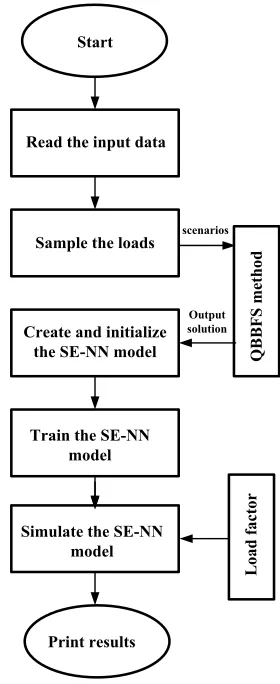
In our approach, we used an efficient method for solving the power flow called quadratic based backward/forward sweep (QBBFS) [31]. Unlike the traditional quadratic based methods that cannot be employed for the unbalanced systems, the QBBFS method accommodates multiphase systems and different load types. Although QBBFS is an efficient method, it requires a long time to estimate the state of the grid. The QBBFS method is used for the large system, where the backward sweep is used for calculating the branch currents from the far ends, and the forward sweep is used for calculating the voltages from the slack bus. In QBBFS, the iteration is repeated until reaching to high convergence rate. Fig. 3 shows the steps of estimation the real-time voltage using a neural network model.

C. The Solution Steps

1. Read the data inputs from the load profiles.

2. Sample the input data and solve it using QBBFS method. 3. Redirect the QBBFS outputs (voltages or re/active power) to the

SE-NN model.

4. Create the SE-NN model using the feed forward neural network with initial parameters and Levenberg-Marquardt algorithm that has high efficiency.

5. Train the SE-NN model with the initialize network created and training parameters. In the training process, the actual QBBFS output is compared with the measured SE-NN output until the network performance goal is met (maximum 300 epochs, minimum 5% gradient and 1e-3 goal error). If the goal is not met, the weights and biases are updated with the learning machine rate until the error is equal or less than the network goal.

6. Once the model is trained, it would be able to simulate the output results for any change in the input data set (Load Factor). 7. Finally, the results are printed.

The proposed algorithm overcomes the high complexity of the computational methods. The function of the QBBFS method is to solve the power flow and redirect the output for training the network, once the network model is learned, the model is saved and used to simulate and reproduce the output rapidly and accurately for any new input data without the need for the QBBFS method.

IV. Assessing the Accuracy of the Proposed Method

To validate the accuracy of the proposed method, we compute the difference between the actual output using the QBBFS method and the network output using the SE-NN method. To perform this we compute different types of errors such as the mean square error (MSE) which is expressed as the average of the square difference between the actual output and the network output.

(8)

where M is the size of the duration, i denotes to the bus number (for voltage calculations) or the line number (for losses calculations), and X represents the state estimation (e.g., voltage, active or reactive power), is the QBBFS output, and is the SE-NN output. In equation (9) we calculate the square root of the mean of the squared difference between actual and estimated output which is called the root mean square error (RMSE). The maximum value of the absolute difference between actual and measured output which is called the maximum absolute error (MAE)) is expressed in (10). The mean absolute percentage error (MAPE) and the sum of the squared error (SSE) are expressed in (11) and (12), respectively.

(9)

(10)

scenarios

QBBFS method

Start

Read the input data

Sample the loads

Create and initialize the SE-NN model

Train the SE-NN model

Simulate the SE-NN model

Print results

Load factor

Output solution

(4)

(11)

(12)

The maximum values of the previous errors are computed to evaluate the accuracy of the proposed method.

V. Results and Discussions

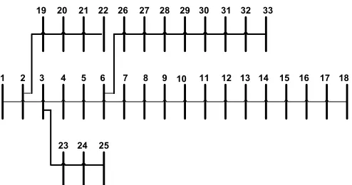
This section presents the results of state estimation using the proposed SE-NN method in smart grids. This method has been implemented at 2.20GHZ CPU, Intel Core i5 and 4GB RAM using MATLAB. The test is applied to a 33-bus distribution system as shown in Fig. 4. To assess the performance of the proposed method, two training datasets with different sizes are provided (200 and 1440 data resolutions). To validate the accuracy of the proposed method, the following steps are carried out:

• We analyze the state estimation of the smart grid using two training datasets (200 and 1440 samples).

• We compare the proposed SE-NN method and the exact QBBFS method.

• To validate the accuracy of the proposed method, we calculate MSE, RMSE, MAE, MAPE, and MSSE.

• For outlining the contribution of the proposed method, we calculate the execution time for producing the SE-NN output and then compare it with the execution time of the exact one.

1 2 3 4 5 6 7 8 9 10 11 12 13 14 15 31 32 33 28 29 30

22 26 27 19 20 21

23 24 25

16 17 18

Fig. 4. The single-line diagram of the 33-bus distribution system.

A. Voltage Estimation

Fig. 5 shows a comparison between the actual voltages computed by the exact power flow method and the estimated voltage computed by the SE-NN method with data resolution of 200 for three buses (10, 25 and 32 buses). We use the per unit expression as a fraction of the base unit for simplifying the calculations. The other dataset is applied, which is a day data per minutes containing 1440 samples (24*60). Fig. 6 shows the estimated and exact voltages at 10, 25, and 32 buses. It is important to note that there is a little difference between the actual and estimated voltages for both data resolutions. This implies that the proposed method gives very accurate estimations of voltages.

0.2 0.3 0.4 0.5 0.6 0.7 0.8 0.9 1 1.1 1.2 11.4

11.6 11.8 12 12.2 12.4 12.6 12.8

Load Factor

V

ol

tages

(k

v)

Actual Voltage Estimated Voltage

(a)

0.2 0.3 0.4 0.5 0.6 0.7 0.8 0.9 1 1.1 1.2 12.15

12.2 12.25 12.3 12.35 12.4 12.45 12.5 12.55 12.6

Load Factor

V

ol

tages

(k

v)

(b)

0.2 0.3 0.4 0.5 0.6 0.7 0.8 0.9 1 1.1 1.2 11.2

11.4 11.6 11.8 12 12.2 12.4 12.6 12.8

Load Factor

V

ol

tages

(k

v)

(c)

(5)

0.2 0.3 0.4 0.5 0.6 0.7 0.8 0.9 1 1.1 1.2 11.4

11.6 11.8 12 12.2 12.4 12.6 12.8

Load Factor

V

ol

tages

(k

v)

(a)

0.2 0.3 0.4 0.5 0.6 0.7 0.8 0.9 1 1.1 1.2 12.15

12.2 12.25 12.3 12.35 12.4 12.45 12.5 12.55 12.6

Load Factor

V

ol

tages

(k

v)

(b)

0.2 0.3 0.4 0.5 0.6 0.7 0.8 0.9 1 1.1 1.2 11.2

11.4 11.6 11.8 12 12.2 12.4 12.6 12.8

Load Factor

V

ol

tages

(k

v)

(c)

Fig. 6. The actual and estimated voltages magnitudes with 1440 data resolution of different buses (a) bus 10, (b) bus 25, and (c) bus 32.

B. Active Power Estimation

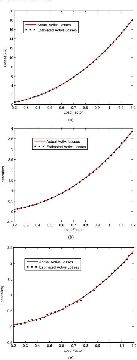
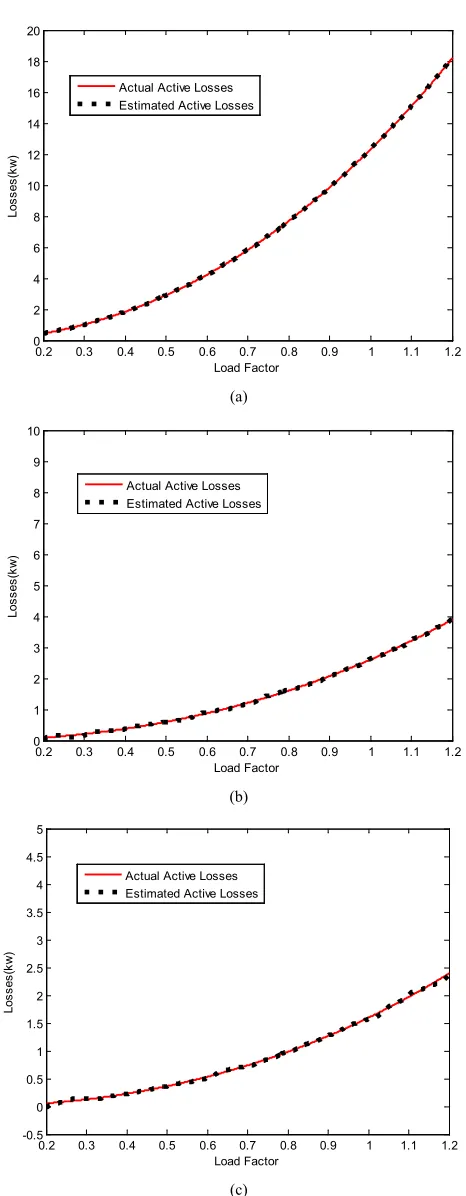
The same data resolutions are applied for computing active power losses. We choose three lines (1, 25 and 30) for testing the datasets. The active power losses for the three lines with 200 and 1440 data sets are shown in Fig. 7 and Fig. 8, respectively. The total active losses for all the system are also shown in Fig. 9 for 200 and 1440 data resolutions.

We notice a strong match between the losses computed by the proposed method and the exact one.

0.2 0.3 0.4 0.5 0.6 0.7 0.8 0.9 1 1.1 1.2 0

2 4 6 8 10 12 14 16 18 20

Load Factor

Lo

ss

es

(k

w

)

Actual Active Losses Estimated Active Losses

(a)

0.2 0.3 0.4 0.5 0.6 0.7 0.8 0.9 1 1.1 1.2 -0.5

0 0.5 1 1.5 2 2.5 3 3.5 4

Load Factor

Lo

ss

es

(k

w

)

(b)

0.2 0.3 0.4 0.5 0.6 0.7 0.8 0.9 1 1.1 1.2 -0.5

0 0.5 1 1.5 2 2.5

Load Factor

Lo

ss

es

(k

w

)

(c)

(6)

0.2 0.3 0.4 0.5 0.6 0.7 0.8 0.9 1 1.1 1.2 0

2 4 6 8 10 12 14 16 18 20

Load Factor

Lo

ss

es

(k

w

)

(a)

0.2 0.3 0.4 0.5 0.6 0.7 0.8 0.9 1 1.1 1.2 0

1 2 3 4 5 6 7 8 9 10

Load Factor

Lo

ss

es

(k

w

)

(b)

0.2 0.3 0.4 0.5 0.6 0.7 0.8 0.9 1 1.1 1.2 -0.5

0 0.5 1 1.5 2 2.5 3 3.5 4 4.5 5

Load Factor

Lo

ss

es

(k

w

)

(c)

Fig. 8. The actual and estimated active power loss magnitudes with 1440 data resolution of different lines (a) line 1, (b) line 25, and (c) line 30.

0.2 0.3 0.4 0.5 0.6 0.7 0.8 0.9 1 1.1 1.2 0

50 100 150 200 250 300 350

Load Factor

Lo

ss

es

(k

w

)

(a)

0.2 0.3 0.4 0.5 0.6 0.7 0.8 0.9 1 1.1 1.2 0

50 100 150 200 250 300 350

Load Factor

Lo

ss

es

(k

w

)

(b)

Fig. 9. The total actual and estimated active losses magnitudes for the two data resolutions (a) 200 data resolution, and (b) 1440 data resolution.

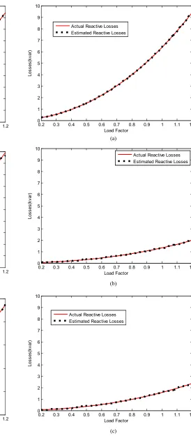
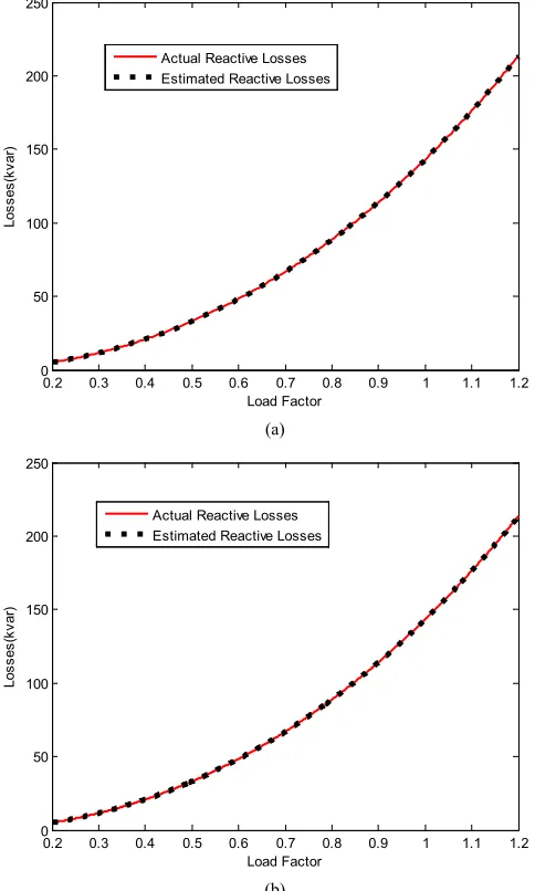
C. Reactive Power Estimation

(7)

0.2 0.3 0.4 0.5 0.6 0.7 0.8 0.9 1 1.1 1.2 0

1 2 3 4 5 6 7 8 9 10

Load Factor

Lo

ss

es

(k

va

r)

Actual Reactive Losses Estimated Reactive Losses

(a)

0.2 0.3 0.4 0.5 0.6 0.7 0.8 0.9 1 1.1 1.2 0

0.2 0.4 0.6 0.8 1 1.2 1.4 1.6 1.8 2

Load Factor

Lo

ss

es

(k

va

r)

(b)

0.2 0.3 0.4 0.5 0.6 0.7 0.8 0.9 1 1.1 1.2 0

0.5 1 1.5 2 2.5

Load Factor

Lo

ss

es

(k

va

r)

(c)

Fig. 10. The actual and estimated reactive power loss magnitudes with 200 data resolution of different lines (a) line 1, (b) line 25, and (c) line 30.

0.2 0.3 0.4 0.5 0.6 0.7 0.8 0.9 1 1.1 1.2 0

1 2 3 4 5 6 7 8 9 10

Load Factor

Lo

ss

es

(k

va

r)

(a)

0.2 0.3 0.4 0.5 0.6 0.7 0.8 0.9 1 1.1 1.2 0

1 2 3 4 5 6 7 8 9 10

Load Factor

Lo

ss

es

(k

va

r)

(b)

0.2 0.3 0.4 0.5 0.6 0.7 0.8 0.9 1 1.1 1.2 0

1 2 3 4 5 6 7 8 9 10

Load Factor

Lo

ss

es

(k

va

r)

(c)

(8)

0.2 0.3 0.4 0.5 0.6 0.7 0.8 0.9 1 1.1 1.2 0

50 100 150 200 250

Load Factor

Lo

ss

es

(k

va

r)

(a)

0.2 0.3 0.4 0.5 0.6 0.7 0.8 0.9 1 1.1 1.2 0

50 100 150 200 250

Load Factor

Lo

ss

es

(k

va

r)

(b)

Fig. 12. The total actual and estimated reactive losses magnitudes for the two data resolutions (a) 200 data resolution, and (b) 1440 data resolution.

D. Performance Comparison

To assess the validity of the proposed method, the different errors are computed for comparing the QBBFS and SE-NN outputs of voltages and re/active power loss. Table I demonstrates the maximum value of the MSE, RMSE, MAE, MAPE, and SSE at all busses for 200 samples. As we can see, the values of errors are very small. In the case of increasing data size to 1440, errors are still small, as illustrated in Table II. This demonstrates the high accuracy of the proposed method.

TABLE I. Maximum Values of Errors at 200 Data Eesolutions

Errors Voltages Active losses Reactive losses

MMSE 4.0765e-04 9.5776e-04 9.3902e-04

MRMSE 0.0202 0.0309 0.0306

MAE 0.2164 0.2440 0.2354

MAPE 5.8776e-04 0.3169 0.3074

MSSE 0.0819 0.1925 0.1887

TABLE II. Maximum Values of Errors at 1440 Data Resolutions

Errors Voltages Active losses Reactive losses

MMSE 1.2011e-04 9.9229e-04 9.9254e-04

MRMSE 0.0110 0.0312 0.0315

MAE 0.0324 0.2638 0.1735

MAPE 6.4528e-04 0.5831 0.2910

MSSE 0.1730 1.4289 1.4293

For further illustrating the effectiveness and contribution of the SE-NN method, the required time for producing the output from QBBFS and SE-NN is compared. With the 200-data resolution, the QBBFS method takes longer execution time (around 16 sec) than the SE-NN method which is not exceeding 0.5 sec, as shown in Table III. For the data size of 1440, a slight change occurs in the execution time of the SE-NN (less than 0.6 sec), while the execution time of QBBFS increases dramatically (more than 115 sec), as shown in Table IV. It worth noting that the computational performance of the SE-NN method is not affected by increasing the data size as in the case of the iterative method.

TABLE III. Execution Time with 200 Data Resolution

Method Voltages Active losses Reactive losses

QBBFS 16.546066 16.181725 16.247039

SE-NN 0.461741 0.223520 0.437750

TABLE IV. Execution Time with 1440 Data Resolution

Method Voltages Active losses Reactive losses

QBBFS 128.972066 115.736379 116.249624

SE-NN 0.589995 0.239677 0.471077

VI. Conclusion

In this paper, the SE-NN method has been proposed for estimating the state of smart grid systems. The proposed method utilizes the feed-forward neural network to determine the state estimation of smart grids. The existing power flow methods take very long execution time, while the proposed method estimates the state at any point in a quick and accurate way. The experiments have been carried out at two different training sets (200 and 1440 data resolution). The proposed method has been compared with the QBBFS method for validation. SE-NN has the ability to estimate the state of smart grid rapidly with high accuracy rate. The proposed method can be a helpful tool for system operators for monitoring the real-time operation of smart grids. The future work will be directed to simulating large-scale distribution systems with renewable energy sources, such as photovoltaic and wind generation systems. In addition, we will use deep learning methods to estimate the state of smart grids

References

[1] C. González García, D. Meana Llorián, C. Pelayo G-Bustelo, and J. M. Cueva-Lovelle, “A review about Smart Objects, Sensors, and Actuators,”

International Journal of Interactive Multimedia and Artificial Intelligence, vol. 4, no. 3, pp. 7-10, 2017.

(9)

3114–3115.

[3] T. Halder, “A smart grid,” in 2014 6th IEEE Power India International Conference (PIICON), 2014, pp. 1–6.

[4] V. C. Gungor et al., “Smart Grid Technologies: Communication Technologies and Standards,” IEEE Trans. Ind. Informatics, vol. 7, no. 4, pp. 529–539, Nov. 2011.

[5] H. Farhangi, “The path of the smart grid,” IEEE Power Energy Mag., vol. 8, no. 1, pp. 18–28, Jan. 2010.

[6] M. Abdel-Nasser and K. Mahmoud, “Accurate photovoltaic power forecasting models using deep LSTM-RNN,” Neural Comput. Appl., pp. 1–14, Oct. 2017.

[7] H. Mortazavi, H. Mehrjerdi, M. Saad, S. Lefebvre, D. Asber, and L. Lenoir, “A Monitoring Technique for Reversed Power Flow Detection With High PV Penetration Level,” IEEE Trans. Smart Grid, vol. 6, no. 5, pp. 2221–2232, Sep. 2015.

[8] A. P. Kenneth and K. Folly, “Voltage Rise Issue with High Penetration of Grid Connected PV,” IFAC Proc. Vol., vol. 47, no. 3, pp. 4959–4966, 2014.

[9] G. K. Ari and Y. Baghzouz, “Impact of high PV penetration on voltage regulation in electrical distribution systems,” in 2011 International Conference on Clean Electrical Power (ICCEP), 2011, pp. 744–748.

[10] W. Tinney and C. Hart, “Power Flow Solution by Newton’s Method,”

IEEE Trans. Power Appar. Syst., vol. PAS-86, no. 11, pp. 1449–1460, Nov. 1967.

[11] K. Mahmoud and M. Abdel-Nasser, “Efficient SPF approach based on regression and correction models for active distribution systems,” IET Renew. Power Gener., vol. 11, no. 14, pp. 1778–1784, Dec. 2017.

[12] Y. Zhang, R. Madani, and J. Lavaei, “Power system state estimation with line measurements,” in 2016 IEEE 55th Conference on Decision and Control (CDC), 2016, pp. 2403–2410.

[13] H. Hooshyar and L. Vanfretti, “Power flow solution for multiphase unbalanced distribution networks with high penetration of photovoltaics,” in 2013 8th International Conference on Electrical and Electronics Engineering (ELECO), 2013, pp. 167–171.

[14] R. Dugan, U. S. A. Epri, and G. Ramos, “Harmonics Analysis Using Sequential-Time Simulation for Addressing,” 23th International Conference on Electricity Distribution (CIRED), pp. 15–18, 2015.

[15] T. Adefarati and R. C. Bansal, “Integration of renewable distributed generators into the distribution system: a review.,” IET Renew. Power Gener., vol. 10, no. 7, pp. 873–884, 2016.

[16] Danling Cheng, B. Mather, R. Seguin, J. Hambrick, and R. P. Broadwater, “PV impact assessment for very high penetration levels,” in 2015 IEEE 42nd Photovoltaic Specialist Conference (PVSC), 2015, pp. 1–6.

[17] C. D. López, “Thesis: Shortening time-series power flow simulations for cost-benefit analysis of LV network operation with PV feed-in,” 2015.

[18] K. S. Narendra and K. Parthasarathy, “Identification and control of dynamical systems using neural networks,” IEEE Trans. Neural Networks, vol. 1, no. 1, pp. 4–27, Mar. 1990.

[19] M. Al Shamisi, A. Assi, and H. Hejase, “Using MATLAB to Develop Artificial Neural Network Models for Predicting Global Solar Radiation in Al Ain City–UAE,” Intechopen.Com, pp. 219–238, 2009.

[20] P. Siano, C. Cecati, H. Yu, and J. Kolbusz, “Real Time Operation of Smart Grids via FCN Networks and Optimal Power Flow,” IEEE Trans. Ind. Informatics, vol. 8, no. 4, pp. 944–952, Nov. 2012.

[21] H. Le Nguyen, “Newton-Raphson method in complex form [power system load flow analysis],” IEEE Trans. Power Syst., vol. 12, no. 3, pp. 1355– 1359, 1997.

[22] J.-H. Teng, “A modified Gauss–Seidel algorithm of three-phase power flow analysis in distribution networks,” Int. J. Electr. Power Energy Syst., vol. 24, no. 2, pp. 97–102, Feb. 2002.

[23] B. N. Rao and R. Inguva, “Power System State Estimation Using Weighted Least Squares ( WLS ) and Regularized Weighted Least Squares ( RWLS ) Method,” International Journal of Engineering Research and Applications, vol. 6, no. 5, pp. 1–6, 2016.

[24] A. Primadianto and C.-N. Lu, “A Review on Distribution System State Estimation,” IEEE Trans. Power Syst., vol. 32, no. 5, pp. 3875-3883, 2016.

[25] C. Muscas, M. Pau, P. A. Pegoraro, S. Sulis, F. Ponci, and A. Monti, “Multiarea Distribution System State Estimation,” IEEE Transactions on Instrumentation and Measurement, vol. 64, no. 5, pp.1140-1148, 2015.

[26] J. Deboever, X. Zhang, M. J. Reno, R. J. Broderick, S. Grijalva, and F. Therrien “Challenges in reducing the computational time of

QSTS simulations for distribution system analysis,” Sandia National Laboratories, SAND2017-5743, 2017.

[27] H. Ramchoun, M. Amine, J. Idrissi, Y. Ghanou, and M. Ettaouil, “Multilayer Perceptron: Architecture Optimization and Training,” International Journal of Interactive Multimedia and Artificial Intelligence, vol. 4, no. 1, pp. 26-30, 2016.

[28] J. R. Machado Fernández and J. C. Bacallao Vidal, “Improved Shape Parameter Estimation in K Clutter with Neural Networks and Deep Learning,” International Journal of Interactive Multimedia and Artificial Intelligence, vol. 3, no. 7, pp. 96-103, 2016.

[29] K. Haddouch, K. Elmoutaoukil, and M. Ettaouil, “Solving the Weighted Constraint Satisfaction Problems Via the Neural Network Approach,”

International Journal of Interactive Multimedia and Artificial Intelligence, vol. 4, no. 1, pp. 56-60, 2016.

[30] S. C. Huang and Y.-F. Huang, “Learning algorithms for perceptions using back-propagation with selective updates,” IEEE Control Syst. Mag., vol. 10, no. 3, pp. 56–61, Apr. 1990.

[31] N. Yorino and K. Mahmoud, “Robust quadratic-based BFS power flow method for multi-phase distribution systems,” IET Gener. Transm. Distrib., vol. 10, no. 9, pp. 2240–2250, 2016.

Mohamed Abdel-Nasser

Dr. Mohamed Abdel-Nasser received his B.Sc and M.Sc degrees in Electrical Engineering from Aswan University (Egypt) and his Ph.D in Computer Engineering from Universitat Rovira i Virgili (Spain) in 2009, 2013, and 2016, respectively. He received the 2017 Marc Esteva Vivanco prize to the best PhD dissertation on Artificial Intelligence (Spain, 2017). His doctoral thesis was on the analysis of breast cancer images. He is currently an Assistant Professor at the Department of Electrical Engineering, Faculty of Engineering, Aswan University, Aswan, Egypt. He has participated in several projects funded by the Government of Spain and the Government of Egypt. He has published more than 40 papers in international conferences and journals. His research interests include the application of machine learning and deep learning to several real-world problems, including breast cancer detection, diabetic retinopathy image analysis, skin cancer detection, smart grid analysis, time-series forecasting, wireless communication, wireless link quality estimation and sediment modeling and estimation in Nasser Lake, Egypt.Dr. Abdel-Nasser is actively serving as a Reviewer to several journal and conference publications including IEEE Transactions. He is one of the founders of the International Conference on Innovative Trends in Computer Engineering.

Heba Kashef

Heba Kashef received the B.Sc. degree in Electrical Engineering from the Faculty of Engineering, Aswan University, Aswan, Egypt, in 2012. Her interests include machine learning and smart grid analysis.

Karar Mahmoud