A Bayesian Framework for Learning Rule Sets for Interpretable
Classification
Tong Wang TONG-WANG@UIOWA.EDUUniversity of Iowa
Cynthia Rudin CYNTHIA@CS.DUKE.EDUDuke University
Finale Doshi-Velez FINALE@SEAS.HARVARD.EDUHarvard University
Yimin Liu LIUYIMIN2000@GMAIL.COMEdward Jones
Erica Klampfl EKLAMPFL@FORD.COMFord Motor Company
Perry MacNeille PMACNEIL@FORD.COMFord Motor Company
Editor:Maya Gupta
Abstract
We present a machine learning algorithm for building classifiers that are comprised of asmall num-ber ofshortrules. These are restricted disjunctive normal form models. An example of a classifier of this form is as follows: If X satisfies (conditionAAND conditionB) OR (conditionC) OR · · ·,thenY = 1. Models of this form have the advantage of being interpretable to human experts since they produce a set of rules that concisely describe a specific class. We present two proba-bilistic models with prior parameters that the user can set to encourage the model to have a desired size and shape, to conform with a domain-specific definition of interpretability. We provide a scal-able MAP inference approach and develop theoretical bounds to reduce computation by iteratively pruning the search space. We apply our method (Bayesian Rule Sets –BRS) to characterize and predict user behavior with respect to in-vehicle context-aware personalized recommender systems. Our method has a major advantage over classical associative classification methods and decision trees in that it does not greedily grow the model.
Keywords: disjunctive normal form, statistical learning, data mining, association rules, inter-pretable classifier, Bayesian modeling
1. Introduction
When applying machine learning models to domains such as medical diagnosis and customer behav-ior analysis, in addition to a reliable decision, one would also like to understand how this decision is generated, and more importantly, what the decision says about the data itself. For classification tasks specifically, a few summarizing and descriptive rules will provide intuition about the data that can directly help domain experts understand the decision process.
Our goal is to construct rule set models that serve this purpose: these models provide predictions and also descriptions of a class, which are reasons for a prediction. Here is an example of a rule set model for predicting whether a customer will accept a coupon for a nearby coffee house, where the coupon is presented by their car’s mobile recommendation device:
if a customer (goes to coffee houses≥once per month AND destination=no urgent place AND passenger6=kids)
OR (goes to coffee houses ≥once per month AND the time until coupon expires= one day)
then
predict the customer will accept the coupon for a coffee house.
This model makes predictions and provides characteristics of the customers and their contexts that lead to an acceptance of coupons.
Formally, a rule set model consists of a set ofrules, where each rule is a conjunction of condi-tions. Rule set models predict that an observation is in the positive class when at least one of the rules is satisfied. Otherwise, the observation is classified to be in the negative class. Rule set models that have a small number of conditions are useful as non-black-box (interpretable) machine learn-ing models. Observations come with predictions and also reasons (e.g., this observation is positive
becauseit satisfies a particular rule).
This form of model appears in various fields with various names. First, they are sparse disjunc-tive normal form (DNF) models. In operations research, there is a field called “logical analysis of data" (Boros et al., 2000; Crama et al., 1988), which constructs rule sets based on combinatorics and optimization. Similar models are called “consideration sets" in marketing (see, e.g., Hauser et al., 2010), or “disjunctions of conjunctions." Consideration sets are a way for humans to handle information overload. When confronted with a complicated decision (such as which television to purchase), the theory of consideration sets says that humans tend to narrow down the possibilities of what they are willing to consider into a small disjunction of conjunctions (“only consider TV’s that are small AND inexpensive, OR large and with a high display resolution"). In PAC learning, the goal is to learn rule set models when the data are non-noisy, meaning there exists a model within the class that perfectly classifies the data. The field of “rule learning" aims to construct rule set models. We prefer the terms “rule set" models or “sparse DNF" for this work as our goal is to create interpretable models for non-experts, which are not necessarily consideration sets, not other forms of logical data analysis, and pertain to data sets that are potentially noisy, unlike the PAC model.
For many decisions, the space of good predictive models is often large enough to include very simple models (Holte, 1993). This means that there may exist very sparse but accurate rule set models; the challenge is determining how to find them efficiently. Greedy methods used in previous works (Malioutov and Varshney, 2013; Pollack et al., 1988; Friedman and Fisher, 1999; Gaines and Compton, 1995), where rules are added to the model one by one, do not generally produce high-quality sparse models.
We create a Bayesian framework for constructing rule sets, which provides priors for control-ling the size and shape of a model. These methods strike a nice balance between accuracy and interpretability through user-adjustable Bayesian prior parameters. To control interpretability, we introduce two types of priors on rule set models, one that uses beta-binomials to model the rule selecting process, called BRS-BetaBinomial, and one that uses Poisson distributions to model rule generation, called BRS-Poisson. Both can be adjusted to suit a domain-specific notion of inter-pretability; it is well-known that interpretability comes in different forms for different domains (Martens and Baesens, 2010; Martens et al., 2011; Huysmans et al., 2011; Allahyari and Lavesson, 2011; Rüping, 2006; Freitas, 2014).
fre-quent in the database and as the search continues, the bound becomes tighter and further reduces the search space. This greatly reduces computational complexity and allows the problem to be solved in practical settings. The theoretical result takes advantage of the strength of the Bayesian prior.
Our applied interest is to understand user responses to personalized advertisements that are chosen based on user characteristics, the advertisement, and the context. Such systems are called
context-aware recommender systems(see surveys Adomavicius and Tuzhilin, 2005, 2008; Verbert et al., 2012; Baldauf et al., 2007, and references therein). One major challenge in the design of recommender systems, reviewed in Verbert et al. (2012), is theinteraction challenge: users typi-cally wish to knowwhy certain recommendations were made. Our work addresses precisely this challenge: our models provide rules in data that describe conditions for a recommendation to be accepted.
The main contributions of our paper are as follows:
• We propose a Bayesian approach for learning rule set (DNF) classifiers. This approach in-corporates two important aspects of performance, accuracy, and interpretability, and balance between them via user-defined parameters. Because of the foundation in Bayesian methodol-ogy, the prior parameters are meaningful; they represent the desired size and shape of the rule set.
• We derive bounds on the support of rules and number of rules in a MAP solution. These bounds are useful in practice because they safely (and drastically) reduce the solution space, improving computational efficiency. The bound on the size of a MAP model guarantees a sparse solution if prior parameters are chosen to favor smaller sets of rules. More importantly, the bounds become tighter as the search proceeds, reducing the search space until the search finishes.
• The simulation studies demonstrate the efficiency and reliability of the search procedure. Losses in accuracy usually result from a misspecified rule representation, not generally from problems with optimization. Separately, using publicly available data sets, we compare rule set models to interpretable and uninterpretable models from other popular classification meth-ods. Our results suggest that BRS models can achieve competitive performance, and are particularly useful when data are generated from a set of underlying rules.
• We study in-vehicle mobile recommender systems. Specifically, we used Amazon Mechan-ical Turk to collect data about users interacting with a mobile recommendation system. We used rule set models to understand and analyze consumers’ behavior and predict their re-sponse to different coupons recommended in different contexts. We were able to generate interpretable results that can help domain experts better understand their customers.
A shorter version of this work appeared at the International Conference on Data Mining (Wang et al., 2016).
2. Related Work
The models we are studying have different names in different fields: “disjunctions of conjunctions" in marketing, “classification rules" in data mining, “disjunctive normal forms" (DNF) in artificial intelligence, and “logical analysis of data" in operations research. Learning logical models of this form has an extensive history in various settings. The LAD techniques were first applied to binary data in (Crama et al., 1988) and were later extended to non-binary cases (Boros et al., 2000). In par-allel, Valiant (1984) showed that DNFs could be learned in polynomial time in the PAC (probably approximately correct - non-noisy) setting, and recent work has improved those bounds via polyno-mial threshold functions (Klivans and Servedio, 2001) and Fourier analysis (Feldman, 2012). Other work studies the hardness of learning DNF (Feldman, 2006). None of these theoretical approaches considered the practical aspects of building asparsemodel with realistic noisy data.
In the meantime, the data-mining literature has developed approaches to building logical con-junctive models. Associative classification and rule learning methods (e.g., Ma et al., 1998; Li et al., 2001; Yin and Han, 2003; Chen et al., 2006; Cheng et al., 2007; McCormick et al., 2012; Rudin et al., 2013; Dong et al., 1999; Michalski, 1969; Clark and Niblett, 1989; Frank and Wit-ten, 1998) mine for frequent rules in the data and combine them in a heuristic way, where rules are ranked by an interestingness criteria. Some of these methods, like CBA, CPAR and CMAR (Li et al., 2001; Yin and Han, 2003; Chen et al., 2006; Cheng et al., 2007) still suffer from a huge number of rules. Inductive logic programming (Muggleton and De Raedt, 1994) is similar, in that it mines (potentially complicated) rules and takes the simple union of these rules as the rule set, rather than optimizing the rule set directly. This is a major disadvantage over the type of approach we take here. Another class of approaches aims to construct rule set models by greedily adding the conjunction that explains the most of the remaining data (Malioutov and Varshney, 2013; Pollack et al., 1988; Friedman and Fisher, 1999; Gaines and Compton, 1995; Cohen, 1995). Thus, again, these methods do not directly aim to produce globally optimal conjunctive models.
There are few recent techniques that do aim to fully learn rule set models. Hauser et al. (2010); Goh and Rudin (2014) applied integer programming approaches to solving the full problems but would face a computational challenge for even moderately sized problems. There are several branch-and-bound algorithms that optimize different objectives than ours (e.g., Webb, 1995). Ri-jnbeek and Kors (2010) proposed an efficient way to exhaustively search for short and accurate decision rules. That work is different than ours in that it does not take a generative approach, and their global objective does not consider model complexity, meaning they do not have the same ad-vantage of reduction to a smaller problem that we have. Methods that aim to globally find decision lists or rule lists can be used to find optimal DNF models, as long as it is possible to restrict all of the labels in the rule list (except the default) to the same value. A rule list where all labels except the default rule are the same value is exactly a DNF formula. We are working on extending the CORELS algorithm (Angelino et al., 2017) to handle DNF.
One could extend any method for DNF learning of binary classification problems to multi-class multi-classification. A conventional way to directly extend a binary multi-classifier is to decompose the multi-class problem into a set of two-class problems. Then for each binary classification problem, one could build a separate BRS model, e.g., by the one-against-all method. One would generate different rule sets for each class. For this approach, the issue of overlapping coverage of rule sets for different classes is handled, for instance, by an error correcting output codes (Schapire, 1997).
The main application we consider is in-vehicle context-aware recommender systems. The most similar works to ours include that of Baralis et al. (2011), who present a framework that discovers relationships between user context and services using association rules. Lee et al. (2006) create in-terpretable context-aware recommendations by using a decision tree model that considers location context, personal context, environmental context and user preferences. However, they did not study some of the most important factors we include, namely contextual information such as the user’s destination, relative locations of services along the route, the location of the services with respect to the user’s destination, passenger(s) in the vehicle, etc. Our work is related to recommendation systems for in-vehicle context-aware music recommendations (see Baltrunas et al., 2011; Wang et al., 2012), but whether a user will accept a music recommendation does not depend on anything analogous to the location of a business that the user would drive to. The setup of in-vehicle rec-ommendation systems are also different than, for instance, mobile-tourism guides (Noguera et al., 2012; Schwinger et al., 2005; Van Setten et al., 2004; Tung and Soo, 2004) where the user is search-ing to accept a recommendation, and interacts heavily with the system in order to find an acceptable recommendation. The closest work to ours is probably that of Park et al. (2007) who also consider Bayesian predictive models for context aware recommender systems to restaurants. They also con-sider demographic and context-based attributes. They did not study advertising, however, which means they did not consider the locations to the coupon’s venue, expiration times, etc.
3. Bayesian Rule Sets
We work with standard classification data. The data setSconsists of{xn, yn}n=1,...N, whereyn∈ {0,1}withN+positive andN−negative, andxn ∈ X. xnhasJ features. Letarepresent a rule
anda(·)with a corresponding Boolean function
a(·) :X → {0,1}.
a(x)indicates ifxsatisfies rulea. LetAdenote a rule set and letA(·)represent a classifier,
A(x) =
(
1 ∃a∈A, a(x) = 1 0 otherwise.
xis classified as positive if it satisfies at least one rule inA.
Figure 1 shows an example of a rule set. Each rule is a yellow patch that covers a particular area, and the rule applies to the area it covers. In Figure 1, the white oval in the middle indicates the positive class. Our goal is to find a set of rulesAthat covers mostly the positive class, but little of the negative class, while keepingAas a small set of short rules.
Figure 1: Illustration of Rule Sets. Area covered by any of rules is classified as positive. Area not covered by any rules is classified as negative.
We propose two models for the prior, a Beta-Binomial prior and a Poisson prior, which characterize the interpretability from different perspectives. The likelihood ensures that the model explains the data well and ensures good classification performance. We detail the priors and likelihood below.
3.1 Prior
We propose two priors. In the BRS-BetaBinomial model, the maximum lengthL of rules is pre-determined by a user. Rules of the same length are placed into the same rulepool. The model uses
Lbeta priors to control the probabilities of selecting rules from different pools. In a BRS-Poisson model, the “shape” of a rule set, which includes the number of rules and lengths of rules, is decided by drawing from Poisson distributions parameterized with user-defined values. Then the generative process fills it in with conditions by first randomly selecting attributes and then randomly selecting values corresponding to each attribute. We present the two prior models in detail.
3.1.1 BETA-BINOMIAL PRIOR
Rules are drawn randomly from a setA. Assuming the interpretability of a rule is associated with thelengthof a rule (the number of conditions in a rule), the rule spaceAis divided intoL pools indexed by the lengths,Lbeing the maximum length the user allows.
A=∪L
l=1Al. (1)
Then, rules are drawn independently in each pool, and we assume inAleach rule has probabilitypl
to be drawn, which we place a beta prior on. Forl∈ {1, ..., L},
Select a rule fromAl∼Bernoulli(pl) (2) pl∼Beta(αl, βl). (3)
is formalized later within proofs). Our approximate inference technique thus finds and uses high support rules to use withinAl. This effectively makes the beta-binomial model non-parametric.
LetMlnotate the number of rules drawn fromAl,l∈ {1, ..., L}. A BRS modelAconsists of
rules selected from each pool. Then
p(A;{αl, βl}l) = L
Y
l=1
Z
pMll (1−pl)(|Al|−Ml)dpl
=
L
Y
l=1
B(Ml+αl,|Al| −Ml+βl) B(αl, βl)
, (4)
whereB(·)represents a Beta function. Parameters{αl, βl}lgovern the prior probability of selecting
a rule set. To favor smaller models, we would chooseαl, βl such that αlαl+βl is close to 0. In our
experiments, we setαl= 1for alll.
3.1.2 POISSON PRIOR
We introduce a data independent prior for the BRS model. LetM denote the total number of rules inAandLmdenote the lengths of rules form∈ {1, ...M}. For each rule, the length needs to be at
least 1 and at most the number of all attributesJ. According to the model, we first drawM from a Poisson distribution. We then drawLm from truncated Poisson distributions (which only allow
numbers from 1 toJ), to decide the “shape” of a rule set. Then, since we know the rule sizes, we can now fill in the rules with conditions. To generate a condition, we first randomly select the attributes then randomly select values corresponding to each attribute. Letvm,k represent the attribute index
for thek-th condition in the m-th rule,vm,k ∈ {1, ...J}. Kvm,k is the total number of values for
attributevm,k. Note that a “value” here refers to a category for a categorical attribute, or an interval
for a discretized continuous variable. To summarize, a rule set is constructed as follows:
1: Draw the number of rules:M ∼Poisson(λ)
2: form∈ {1, ...M}do
3: Draw the number of conditions inm-th rule:Lm ∼Truncated-Poisson(η), Lm ∈ {1, ...J}
4: Randomly selectLmattributes fromJ attributes without replacement
5: fork∈ {1, ...Lm}do
6: Uniformly at random select a value fromKvm,k values corresponding to attributevm,k
7: end for 8: end for
We define the normalization constantω(λ, η), so the probability of generating a rule setAis
p(A;λ, η) = 1
ω(λ, η)Poisson(M;λ)
M
Y
m=1
Poisson(Lm;η)
1
J Lm
Lm
Y
k=1 1 Kvm,k
. (5)
3.2 Likelihood
LetA(xn)denote the classification outcome forxn, and letyndenote the observed outcome. Recall
thatA(xn) = 1ifxnobeys any of the rulesa∈A. We introduce likelihood parameterρ+to
thatyn= 0whenA(xn) = 0. Thus:
yn|xn, A∼
(
Bernoulli(ρ+) A(xn) = 1
Bernoulli(1−ρ−) A(xn) = 0 ,
withρ+andρ−drawn from beta priors:
ρ+ ∼Beta(α+, β+)andρ−∼Beta(α−, β−). (6)
Based on the classification outcomes, the training data are divided into four cases: true pos-itives (TP = P
nA(xn)yn), false positives (FP = PnA(xn)(1−yn)), true negatives (TN =
P
n(1−A(xn)) (1−yn)) and false negatives (FN=
P
n(1−A(xn))yn). Then, it can be derived
that
p(S|A;α+, β+, α−, β−) =
Z
ρTP+(1−ρ+)FPρTN− (1−ρ−)FNdρ+dρ−
=B(TP+α+,FP+β+) B(α+, β+)
B(TN+α−,FN+β−)
B(α−, β−)
. (7)
According to (6), α+, β+, α−, β− govern the probability that a prediction is correct on training data, which determines the likelihood. To ensure the model achieves the maximum likelihood when all data points are classified correctly, we need ρ+ ≥ 1−ρ+ andρ− ≥ 1−ρ−. So we choose
α+, β+, α−, β−such that α++α+β+ >0.5andα−α+−β− >0.5. Parameter tuning for the prior parame-ters will be shown in experiments section. LetHdenote a set of parameters for a dataS,
H =
α+, β+, α−, β−, θprior ,
whereθpriordepends on the prior model, our goal is to find an optimal rule setA∗ that A∗ ∈arg max
A p(A|S;H). (8)
Solving for a MAP model is equivalent to maximizing
F(A, S;H) = logp(A;H) + logp(S|A;H), (9)
where either of the two priors provided above can be used for the first term, and the likelihood is in (7). We write the objective asF(A), the prior probability of selectingAasp(A), and the likelihood asp(S|A), omitting dependence on parameters when appropriate.
4. Approximate MAP Inference
In this section, we describe a procedure for approximately solving for the maximuma posteriori
(MAP) solution to a BRS model.
Inference becomes easier, however, for our BRS model, due to the computational benefits brought by the Bayesian prior, which can effectively reduce the original problem to a much more manageable size and significantly improve computational efficiency. Below, we detail how to ex-ploit the Bayesian prior to derive useful bounds during any search process. Here we use a stochastic coordinate descent search technique, but the bounds hold regardless of what search technique is used.
4.1 Search Procedure
Given an objective function F(A) over discrete search space of different sets of rules and a
tem-perature schedule function over time steps,T[t] = T1− t Niter
0 , a simulated annealing (Hwang, 1988)
procedure is a discrete time, discrete state Markov Chain where at stept, given the current stateA[t], the next stateA[t+1]is chosen by first randomly selecting a proposal from the neighbors, and the proposal is accepted with probabilitymin
n
1,exp
F(A[t+1])−F(A[t]) T[t]
o
, in order to find an optimal rule setA∗. Our version of simulated annealing is similar also to the-greedy algorithm used in multi-armed bandits (Sutton and Barto, 1998).
Similar to the Gibbs sampling steps used by Letham et al. (2015); Wang and Rudin (2015) for rule-list models, here a “neighboring” solution is a rule set whose edit distance is 1 to the current rule set (one of the rules is different). Our simulated annealing algorithm proposes a new solution via two steps: choosing an action from ADD, CUT and REPLACE, and then choosing a rule to perform the action on.
In the first step, the selection of which rules to ADD, CUT or REPLACE is not chosen uni-formly. Instead, the simulated annealing proposes a neighboring solution that aims to do better than the current model with respect to a randomly chosen misclassified point. At iteration t+ 1, an examplekis drawn from data points misclassified by the current modelA[t]. LetR1(xk)represent
a set of rules thatxk satisfies, and letR0(xk)represent a set of rules that xk does not satisfy. If
examplekis positive, it means the current rule set fails to cover it so we propose a new model that covers example k, by either adding a new rule fromR1(xk)toA[t], or replacing a rule fromA[t]
with a rule fromR1(xk). The two actions are chosen with equal probabilities. Similarly, if example kis negative, it means the current rule set covers wrong data, and we then find a neighboring rule set that covers less, by removing or replacing a rule fromA[t]∩ R0(xk), each with probability 0.5.
In the second step, a rule is chosen to perform the action on. To choose the best rule, we evaluate theprecisionof tentative models obtained by performing the selected action on each candidate rule. This precision is:
Q(A) =
P
iA(xi)yi
P
iA(xi) .
Then a choice is made between exploration, which means choosing a random rule (from the ones that improve on the new point), and exploitation, which means choosing the best rule (the one with the highest precision). We denote the probability of exploration aspin our search algorithm. This randomness helps to avoid local minima and helps the Markov Chain to converge to a global minimum. We detail the three actions below.
• ADD
– With probabilityp, drawzrandomly fromR1(xk). (Explore) – With probability1−p,z= arg max
a∈R1(xk)
Q(A[t]∪a).(Exploit)
2. ThenA[t+1]←A[t]∪z.
• CUT
1. Select a rulezaccording toxk
– With probabilityp, drawzrandomly fromA[t]∩ R0(xk). (Explore) – With probability1−p,z= arg max
a∈A[t]∩R0(xk)
Q(A[t]\a).(Exploit)
2. ThenA[t+1]←A[t]\z.
• REPLACE: first CUT, then ADD.
To summarize: the proposal strategy uses an-greedy strategy to determine when to explore and when to exploit, and when it exploits, the algorithm uses a randomized coordinate descent approach by choosing a rule to maximize improvement.
4.2 Iteratively reducing rule space
Another approach to reducing computation is to directly reduce the set of rules. This dramatically reduces the search space, which is the power set of the set of rules. We take advantage of the Bayesian prior and derive a deterministic bound on MAP BRS models that exclude rules that fail to satisfy the bound.
Since the Bayesian prior is constructed to penalize large models, a BRS model tends to contain a small number of rules. As a small number of rules must cover the positive class, each rule in the MAP model must cover enough observations. We define the number of observations that satisfy a rule as thesupportof the rule:
supp(a) =
N
X
n=1
1(a(xn) = 1). (10)
Removing a rule will yield a simpler model (and a smaller prior) but may lower the likelihood. However, we can prove that the loss in likelihood is bounded as a function of the support. For a rule setAand a rulez∈A, we useA\zto represent a set that contains all rules fromAexceptz, i.e.,
A\z ={a|a∈A, a6=z}.
Define
Υ = β−(N++α++β+−1) (N−+α−+β−)(N++α+−1)
.
Then the following holds:
All proofs in this paper are in Appendix A. This lemma shows that ifΥ≤1, removing a rule with high support lowers the likelihood.
We wish to derive lower bounds on the support of rules in a MAP model. This will allow us to remove (low-support) rules from the search space without any loss in posterior. This will simultaneously yield an upper bound on the maximum number of rules in a MAP model. The bounds will be updated as the search proceeds.
Recall that A[τ]denotes the rule set at timeτ, and letv[t]denote the best solution found until iterationt, i.e.,
v[t]= max
τ≤t F(A [τ]).
We first look at BRS-BetaBinomial models. In a BRS-BetaBinomial model, rules are selected based on their lengths, so there are separate bounds for rules of different lengths, and we notate the upper bounds of the number of rules at steptas{m[lt]}l=1,...,L, wherem[lt]represents the upper bound for the number of rules of lengthl.
We then introduce some notations that will be used in the theorems. LetL∗denote the maximum likelihood of dataS, which is achieved when all data are classified correctly (this holds whenα+> β+andα−> β−), i.e. TP=N+, FP= 0, TN=N−, and FN= 0, giving:
L∗ := max
A p(S|A) =
B(N++α+, β+) B(α+, β+)
B(N−+α−, β−)
B(α−, β−)
. (11)
For a BRS-BetaBinomial model, the following is true.
Theorem 1 Take a BRS-BetaBinomial model with parameters
H ={L, α+, β+, α−, β−,{Al, αl, βl}l=1,..L},
whereL, α+, β+, α−, β−,{αl, βl}l=1,...L ∈ N+,α+ > β+, α− > β− andαl < βl. Define A∗ ∈
arg maxAF(A)andM∗ =|A∗|. IfΥ≤1, we have:∀a∈A∗,supp(a)≥C[t]and
C[t]=
log max l
|Al|−m[t
−1] l +βl m[lt−1]−1+αl
log Υ , (12) where
m[lt]=
logL∗+ logp(∅)−v[t] log |Al|+βl−1
αl+m[lt−1]−1
,
andm[0]l =
j
logL∗−logp(S|∅)
log|Al|+βl−1 αl+|Al|−1
k
andv[0]=F(∅). The size ofA∗is upper bounded by
M∗≤ L
X
In the equation form[lt], p(∅) is the prior of an empty set, which is also the maximum prior for a rule set model, which occurs when we setαl = 1for all l. SinceL∗ andp(∅) upper bound the
likelihood and prior, respectively,logL∗+ logp(∅)upper bounds the optimal objective value. The difference between this value and v[t], the numerator, represents the room for improvement from
the current solution v[t]. The smaller the difference, the smaller the m[lt], and thus the larger the minimum support bound. In the extreme case, when an empty set is the optimal solution, i.e., the likelihood and the prior achieve the upper bound L∗ andp(∅) at the same time, and the optimal solution is discovered at time t, then the numerator becomes zero and m[lt] = 0which precisely refers to an empty set. Additionally, parametersαlandβljointly govern the probability of selecting
rules of lengthl, according to formula (3). Whenαl is set to be small andβlis set to be large,pl
is small sinceE(pl) = αlαl+βl. Therefore the resultingm[lt]is small, guaranteeing that the algorithm
will choose a smaller number of rules overall.
Specifically, at step0when there is nom[lt−1], we setm[lt−1]=|Al|, yielding
m[0]l =
logL∗−logp(S|∅) log|Al|+βl−1
αl+|Al|−1
, (13)
which is the upper bound we obtain before we start learning forA∗. This bound uses an empty set as a comparison model, which is a reasonable benchmark since the Bayesian prior favors smaller models. (It is possible, for instance, that the empty model is actually close to optimal, depending on the prior.) Aslogp(S|∅)increases,m[0]l becomes smaller, which means the model’s maximum possible size is smaller. Intuitively, if an empty set already achieves high likelihood, adding rules will often hurt the prior term and achieve little gain on the likelihood.
Using this upper bound, we get a minimum support which can be used to reduce the search space before simulated annealing begins. Asm[t]decreases, the minimum support increases since the rules need to jointly cover positive examples. Also, if fewer rules are needed it means each rule needs to cover more examples.
Similarly, for BRS-Poisson models, we have:
Theorem 2 Take a BRS-Poisson model with parameters
H ={L, α+, β+, α−, β−, λ, η},
whereL, α+, β+, α−, β− ∈ N+,α+ > β+, α− > β−. DefineA∗ ∈ arg maxAF(A)andM∗ = |A∗|. IfΥ≤1, we have:∀a∈A∗,supp(a)≥C[t]and
C[t]=
log x
M[t] log Υ
, (14)
where
x=
e−ηλmax
n
η 2
Γ(J+ 1), η2J
o
Γ(J+ 1) ,
and
M[t]=
log(Γ(λ+1)λ+1)λ
logλ+1x +
logL∗+ logp(∅)−v[t] logλ+1x
The size ofA∗ is upper bounded by
M∗ ≤M[t].
Similar to Theorem 1, logL∗+ logp(∅)upper bounds the optimal objective value and logL∗+ logp(∅)−v[t]is an upper bound on the room for improvement from the current solutionv[t]. The smaller the bounds becomes, the larger is the minimum support, thus reducing the rule space itera-tively whenever a new maximum solution is discovered.
The algorithm, which applies the bounds above, is given as Algorithm 1.
Algorithm 1 Inference algorithm.
procedureSIMULATEDANNEALING(Niter)
A ←FP-Growth(S)
A[0] ←a randomly generated rule set
Amax←A[0]
fort= 0→Niterdo
A ← {a∈ A,supp(a)≥C[t]}(C[t]is from (12) or (14), depending on the model choice)
S ←misclassified examples byA[t](Find misclassified examples)
(xk, yk)←a random example drawn fromS ifyk= 1then
action←
(
ADD, with probability0.5
REPLACE, with probability0.5
else
action←
(
CUT, with probability0.5
REPLACE, with probability0.5 A[t+1]←action(A, A[t],xk)
Amax←arg max(F(Amax), F(A[t+1]))(Check for improved optimal solution) α = min
n
1,exp
F(A[t+1])−F(A[t]) T[t]
o
(Probability of an annealing move)
A[t+1]←
(
A[t+1], with probabilityα A[t], with probability1−α end for
returnAmax end procedure
4.3 Rule Mining
We mine a set of candidate rulesAbefore running the search algorithm and only search withinA to create an approximate but more computationally efficient inference algorithm. For categorical at-tributes, we consider both positive associations (e.g.,xj=‘blue’) and negative associations (xj=‘not
them, i.e., age<25, age<50 and age<75. We then mine for frequent rules within the set of positive observationsS+. To do this, we use the FP-growth algorithm (Borgelt, 2005), which can in practice be replaced with any desired frequent rule-mining method.
Sometimes for large data sets with many features, even when we restrict the length of rules and the minimum support, the number of generated rules could still be too large to handle, as it can be exponential in the number of attributes. For example, for one of the advertisement data sets, a million rules are generated when the minimum support is 5% and the maximum length is 3. In that case, we use a second criterion to screen for the most potentially usefulM0rules, whereM0is
user-defined and depends on the user’s computational capacity. We first filter out rules on the lower right plane of ROC space, i.e., their false positive rate is greater than true positive rate. Then we use
information gainto screen rules, similarly to other works (Chen et al., 2006; Cheng et al., 2007). For a rulea, the information gain is
InfoGain(S|a) =H(S)−H(S|a), (15)
whereH(S)is the entropy of the data andH(S|a) is the conditional entropy of data that split on rulea. Given a data setS, entropyH(S)is constant; therefore our screening technique chooses the
M0rules that have the smallestH(S|a).
Figure 2: All rules and selected rules on a ROC plane
We illustrate the effect of screening on one of our mobile advertisement data sets. We mined all rules with minimum support 5% and maximum length 3. For each rule, we computed its true positive rate and false positive rate on the training data and plotted it as a dot in Figure 2. The top
5. Simulation Studies
We present simulation studies to show the interpretability and accuracy of our model and the effi-ciency of the simulated annealing procedure. We first demonstrate the effieffi-ciency of the simulated annealing algorithm by searching within candidate rules for a “true rule set" that generates the data. Simulations show that our algorithm can recover the true rule set with high probability within a small number of iterations despite the large search space. We then designed the second set of sim-ulations to study the trade-off between accuracy and simplicity. BRS models may lose accuracy to gain model simplicity when the number of attributes is large. Combining the two simulations studies, we were able to hypothesize that possible losses in accuracy are often due to the choice of model representation as a rule set, rather than simulated annealing. In this section, we choose the BRS-BetaBinomial model for the experiments. BRS-Poisson results would be similar; the only difference is the choice of prior.
5.1 Simulation Study 1: Efficiency of Simulated Annealing
In the first simulation study, we would like to test if simulated annealing is able to recover a true rule set given that these rules are in a candidate rule set, and we would like to know how efficiently simulated annealing finds them. Thus we omit the step of rule mining for this experiment and directly work with generated candidate rules, which we know in this case contains a true rule set.
Let there be N observations,{xn}n=1,...,N and a collection of M candidate rules,{am}m=1,...M.
We can construct anN ×M binary matrix where the entry in then-th row andm-th column is the Boolean functionam(xn) that represents whether then-th observation satisfies them-th rule. Let
the true rule set be a subset of the candidate rules,A∗ ⊂ {am}m=1,...M. The labels{yn}n=1,...N
satisfy
yn=
(
1 ∃a∈A∗, a(xn) = 1
0 otherwise. (16)
We ran experiments with varying N andM. Each time, we first generated anN ×M binary matrix by setting the entries to 1 with probability 0.035, and then selected 20 columns to formA∗. (Values 0.035 and 20 are chosen so that the positive class contains roughly 50% of the observations. We also ensured that the 20 rules do not include each other.) Then{yn}n=1,...N were generated as
above. We randomly assigned lengths from 1 to 5 to{am}m=1,...M. Finally, we ran Algorithm 1 on
the data set. The prior parameters were set as below for all simulations:
αl = 1, βl=|Al|forl= 1, ...,3, α+ =α− = 1000, β+=β−= 1.
For each pair ofN andM, we repeated the experiment 100 times and recorded intermediate output models at different iterations. Since multiple different rule sets can cover the same points, we compared labels generated from the true rule set and the recovered rule set: a label is 1 if the instance satisfies the rule set and 0 otherwise. We recorded the training error for each intermediate output model. The mean and standard deviation of training error rate are plot Figure 3, along with run time to convergence in seconds on the right figure.
Figure 3: Convergence of mean error rate with number of iterations for data with varyingN andM
and running time (in seconds), obtained by the BRS-BetaBinomial.
the size of the rule spaceM affected the search. This is because the strategy based on curiosity and bounds chose the best solution efficiently, regardless of the size of data or the rule space.
More importantly, this study shows that simulated annealing is able to recover a true rule set
A∗, or an equivalent rule set with optimal performance, with high probability, with few iterations.
5.2 Simulation Study 2: Accuracy-Interpretability Trade-off
We observe from the first simulation study that simulated annealing does not tend to cause losses in accuracy. In the second simulation study, we would like to identify whether the rule representation causes losses in accuracy. In this study, we used the rule mining step and directly worked with data {xn}n=1,...,N. Without loss of generality, we assumexn∈ {0,1}J.
In each experiment, we first constructed anN ×J binary matrix{xn}n=1,...N by setting the
entries to 1 with probability 0.5, then randomly generated 20 rules from{xn}n=1,...,N to formA∗
and finally generated labels{yn}n=1,...,N following formula (16). We checked the balance of the
data before pursuing the experiment. The data set was used only if the positive class was within
[30%,70%]of the total data, and otherwise regenerated.
To constrain computational complexity, we set the maximum length of rules to be 7 and then selected the top 5000 rules with highest information gain. Then we performed Algorithm 1 on these candidate rules to generate a BRS modelA˜. Ideally,A˜should be simpler thanA∗, with a possible loss in its accuracy as a trade-off.
To study the influence of the dimensions of data on accuracy and simplicity, we varied N and
J and repeated each experiment 100 times. Figure 4 shows the accuracy and number of rules inA˜
in each experiment. The number of rules inA˜was almost always less than the number of rules in
Figure 4: Accuracy and complexity of output BRS models for data with varyingN andJ, obtained from the BRS-BetaBinomial.
We show in Figure 5 the average training error at different iterations to illustrate the convergence rate. Simulated annealing took less than 50 iterations to converge. Note that it took fewer iterations than simulation study 1 since the error rate curve started from less than 0.5, due to rule pre-screening using information gain.
Figure 5: Convergence of mean error rate with varyingN andJ, obtained by BRS-BetaBinomial.
Figure 4 and Figure 5 both indicate that increasing the number of observations did not affect the performance of the model. BRS is more sensitive to the number of attributes. The largerJ is, the less informative a short rule becomes to describe and distinguish a class in the data set, and the more BRS has to trade-off, in order to keep simple rules within the model.
high dimensional feature spaces. The loss increases with the number of features. This is the price paid for using an interpretable model. There is little price paid for using our optimization method.
6. Experiments
Our main application of interest is mobile advertising. We collected a large advertisement data set using Amazon Mechanical Turk that we made publicly available (Wang et al., 2015), and we tested BRS on other publicly available data sets. We show that our model can generate interpretable results that are easy for humans to understand, without losing too much (if any) predictive accuracy. In situations where the ground truth consists of deterministic rules (similarly to the simulation study), our method tends to perform better than other popular machine learning techniques.
6.1 UCI Data Sets
We test BRS on ten data sets from the UCI machine learning repository (Bache and Lichman, 2013) with different types of attributes; four of them contain categorical attributes, three of them contain numerical attributes and three of them contain both. We performed 5-fold cross validation on each data set. Since our goal was to produce models that are accurate and interpretable, we set the maximum length of rules to be 3 for all experiments. We compared with interpretable algorithms: Lasso (without interaction terms to preserve interpretability), decision trees (C4.5 and CART), and inductive rule learner RIPPER (Cohen, 1995), which produces a rule list greedily and anneals locally afterward. In addition to interpretable models, we also compare BRS with uninterpretable models from random forests and SVM to set a benchmark for expected accuracy on each data set. We used implementations of baseline methods from R packages, and tuned model parameters via 5-fold nested cross validation.
Table 1: Accuracy of each comparing algorithm (mean±std) on ten UCI data sets.
Data
BRS1 BRS2 Lasso C4.5 CART RIPPERRandom SVM
Type Forest
connect-4
Categorical
.76±.01 .75±.01 .70±.00 .83±.00 .69±.01 ———- .86±.00 .82±.00 mushroom 1.00±.00 1.00±.00 .96±.00 1.00±.00 .99±.00 .99±.00 1.00±.00 .93±.00 tic-tac-toe 1.00±.00 1.00±.00 .71±.02 .92±.03 .93±.02 .98±.01 .99±.00 .99±.00 chess .89±.01 .89±.01 .83±.01 .97±.00 .92±.04 .91±.01 .91±.00 .99±.00 magic
Numerical
.80±.02 .79±.01 .76±.01 .79±.00 .77±.00 .78±.00 .78±.01 .78±.01 banknote .97±.01 .97±.01 1.00±.00 .90±.01 .90±.02 .91±.01 .91±.01 1.00±.00 indian-diabetes .72±.03 .73±.03 .67±.01 .66±.03 .67±.01 .67±.02 .75±.03 .69±.01 adult
Mixed
.83±.00 .84±.01 .82±.02 .83±.00 .82±.01 .83±.00 .84±.00 .84±.00 bank-marketing .91±.00 .91±.00 .90±.00 .90±.00 .90±.00 .90±.00 .90±.00 .90±.00 heart .85±.03 .84±.03 .85±.04 .76±.06 .77±.06 .78±.04 .81±.06 .86±.06
Rank of accuracy 2.6±1.7 2.6±1.8 5.4±2.8 4.3±2. 9 5.6±1.8 4.8±1.5 2.7±1.7 2.8±2.2
Table 2: Runtime (in seconds) of each comparing algorithm (mean±std) on ten UCI data sets.
BRS1 BRS2 Lasso C4.5 CART RIPPER Random SVM Forest
connect-4 288.1±22.2 279.1±20.9 0.9±0.0 30.4±0.6 20.5±0.4 ———- 746.6±14.9 1427.8±35.1 mushroom 8.8±1.3 8.18±1.3 0.1±0.0 0.5±0.0 0.6±0.0 1.2±0.1 15.6±0.8 23.5±1.2 tic-tac-toe 1.0±0.0 1.0±0.0 0.0±0.0 0.1±0.0 0.1±0.0 0.3±0.0 1.3±.0.0 0.2±0.0 chess 44.8±8.2 41.6±8.2 0.1±0.0 1.3±0.4 0.3±0.1 50.6±18.0 47.5±1.9 1193.3±79.6 magic 31.3±4.4 29.3±4.4 0.1±0.0 1.4±0.1 2.3±0.2 8.8±1.7 43.5±1.3 139.7±3.2 banknote 1.0±0.1 0.9±0.1 0.0±0.0 0.1±0.0 0.1±0.0 0.2±0.0 1.1±0.0 0.1±0.0 indian-diabetes 0.6±0.1 0.6±0.1 0.0±0.0 0.1±0.0 0.1±0.0 0.2±0.0 0.7±0.0 0.2±0.0 adult 50.2±6.2 47.1±6.2 0.4±0.0 9.8±0.3 10.7±0.4 66.0±8.8 344.4±7.7 174.6±4.7 bank-marketing 55.2±2.7 50.8±2.7 0.4±0.0 11.6±0.6 7.6±0.3 23.9±4.6 320.0±9.8 395.1±28.1 heart 0.5±0.1 0.5±0.1 0.0±0.0 0.1±0.0 0.0±0.0 0.2±0.1 0.3±0.0 0.0±0.0
and the rank of their average performance. Table 2 displays the runtime. BRS1 represents BRS-BetaBinomial and BRS2 represents BRS-Poisson. While BRS models were under strict restriction for interpretability purposes (L = 3), BRS’s performance surpassed that of the other interpretable methods and was on par with uninterpretable models. This is because, firstly, BRS has Bayesian priors that favor rules with a large support (Theorem 1, 2) which naturally avoids overfitting of the data; and secondly, BRS optimizes a global objective while decision trees and RIPPER rely on local greedy splitting and pruning methods, and interpretable versions of Lasso are linear in the base features. Decision trees and RIPPER are local optimization methods and tend not to have the same level of performance as globally optimal algorithms, such as SVM, Random Forests, BRS, etc. The class of rule set models and decision tree models are the same: both create regions within input space consisting of a conjunction of conditions. The difference is the choice of optimization method: global vs. local.
For the tic-tac-toe data set, the positive class can be classified using exactly eight rules. BRS has the capability to exactly learn these conditions, whereas the greedy splitting and pruning methods that are pervasive throughout the data mining literature (e.g., CART, C4.5) and convexified approx-imate methods (e.g., SVM) have difficulty with this. Both linear models and tree models exist that achieve perfect accuracy, but the heuristic splitting/pruning and convexification of the methods we compared with prevented these perfect solutions from being found.
BRS achieves accuracies competitive to uninterpretable models while requiring a much shorter runtime, which grows slowly with the size of the data, unlike Random forest and SVM. This indi-cates that BRS can reliably produce a good model within a reasonable time for large data sets.
6.1.1 PARAMETERTUNING
parameters and how to tune the parameters to get the best performing model. We choose one data set from each category from Table 1.
We fixed the prior parameters αl = 1, βl = |Al|for l = 1, .., L, and only varied likelihood
parameters α+, β+, α−, β− to analyze how the performance changes as the magnitude and ratio of the parameters change. To simplify the study, we took α+ = α− = α, andβ+ = β− = β. We let s = α+β ands was chosen from {100,1000,10000}. We let ρ = α+αβ andρ varied within[0,1]. Here,sandρuniquely defineαandβ. We constructed models for differentsandρ
and plotted the average out-of-sample accuracy assandρ changed in Figure 6 for three data sets representative of categorical, numerical and mixed data types. The X axis representsρand Y axis representss. Accuracies increase as ρincreases, which is consistent with the intuition ofρ+and
ρ−. The highest accuracy is always achieved at the right half of the curve. The performance is less sensitive to the magnitudesand ratioρ, especially whenρ > 0.5. For tic-tac-toe and diabetes, the accuracy became flat onceρbecomes greater than a certain threshold, and the performance was not sensitive toρeither after that point; it is important as it makes tuning the algorithm easy in practice. Generally, takingρclose to 1 leads to a satisfactory output. Table 1 and 2 were generated by models withρ= 0.9ands= 1000.
Figure 6: Parameter tuning experiments. Accuracy vs.ρfor all data sets. X axis representsρand Y axis represents accuracy.
6.1.2 DEMONSTRATION WITHTIC-TAC-TOE DATA
Let us illustrate the reduction in computation that comes from the bounds in the theorems in Section 4. For this demonstration, we chose the tic-tac-toe data set since the data can be classified exactly by eight rules which are naturally an underlying true rule set, and our method recovered the rules successfully, as shown in Table 1. We use BRS-BetaBinomial for this demonstration.
First, we used FP-Growth (Borgelt, 2005) to generate rules. At this step, we find all possible rules with length between 1 to9(the data has 9 attributes) and has minimum support of 1 (the rule’s itemset must appear at least once int the data set). FP-growth generates a total of84429rules. We then set the hyper-parameters as:
αl= 1, βl=|Al|forl= 1, ...,9,
α+=N++ 1, β+=N+, α−=N−+ 1, β−=N−.
We ran Algorithm 1 on this data set. We kept a list of the best solutionsv[t] found until time t
Figure 7: Updated minimum support at different iterations
ten iterations, the minimum support increased from 1 to 9. If, however, we choose a stronger prior for small models by increasingβl to 10 times|Al|for all land keeping all the other parameters
unchanged, then the minimum support increases even faster and reached 13 very quickly. This is consistent with the intuition that if the prior penalizes large models more heavily, the output tends to have a smaller size. Therefore each rule will need to cover more data.
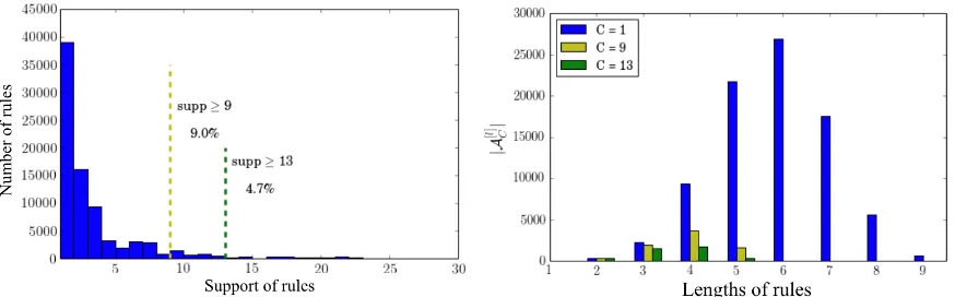
Placing a bound on the minimum support is critical for computation since the number of possible rules decays exponentially with the support, as shown in Figure 8a. As the minimum support is increased, more rules are removed from the original rule space. Figure 8a shows the percentage of rules left in the solution space as the minimum threshold is increased from 1 to 9 and to 13. At a minimum support of 9, the rule space is reduced to 9.0% of its original size; at a minimum support of 13, the rule space is reduced to 4.7%. This provides intuition of the benefit of Theorem 1.
(a) Reduced rule space as the minimum support increases (b) Number of rules of different lengths mined at different minimum support.
Figure 8: Demonstration with Tic-Tac-Toe data set
lev-els. Before any filtering (i.e., C = 1), more than half of the rules have lengths greater than 5. AsC
is increased to 9 and 13, these long rules are almost completely removed from the rule space. To summarize, the strength of the prior is important for computation, and changes the nature of the problem: a stronger prior can dramatically reduce the size of the search space. Any increase in minimum support, that the prior provides, leads to a smaller search by the rule mining method and a smaller optimization problem for the BRS algorithm. These are multiple order-of-magnitude decreases in the size of the problem.
6.2 Application to In-vehicle Recommendation System
For this experiment, our goal was to understand customers’ response to recommendations made in an in-vehicle recommender system that provides coupons for local businesses. The coupons would be targeted to the user in his/her particular context. Our data were collected on Amazon Mechanical Turk via a survey that we will describe shortly. We used Turkers with high ratings (95% or above). Out of 752 surveys, 652 were accepted, which generated 12684 data cases (after removing rows containing missing attributes).
The prediction problem is to predict if a customer is going to accept a coupon for a particular venue, considering demographic and contextual attributes. Answers that the user will drive there ‘right away’ or ‘later before the coupon expires’ are labeled as ‘Y = 1’ and answers ‘no, I do not want the coupon’ are labeled as ‘Y = 0’. We are interested in investigating five types of coupons: bars, takeaway food restaurants, coffee houses, cheap restaurants (average expense below $20 per person), expensive restaurants (average expense between $20 to $50 per person). In the first part of the survey, we asked users to provide their demographic information and preferences. In the second part, we described 20 different driving scenarios (see examples in Appendix B) to each user along with additional context information and coupon information (see Appendix B for a full description of attributes) and asked the user if s/he will use the coupon.
For this problem, we wanted to generate simple BRS models that are easy to understand. So we restricted the lengths of rules and the number of rules to yield very sparse models. Before mining rules, we converted each row of data into an item which is an attribute and value pair. For categorical attributes, each attribute-value pair was directly coded into a condition. Using marital status as an example, ‘marital status is single’ was converted into (MaritalStatus: Single), (MaritalStatus: Not Married partner), and (MaritalStatus: Not Unmarried partner), (MaritalStatus: Not Widowed). For discretized numerical attributes, the levels are ordered, such as: age is ‘20 to 25’, or ‘26 to 30’, etc.; additionally, each attribute-value pair was converted into two conditions, each using one side of the range. For example, age is ‘20 to 25’ was converted into (Age:>=20) and (Age:<=25). Then each condition is a half-space defined by threshold values. For the rule mining step, we set the minimum support to be 5% and set the maximum length of rules to be 4. We used information gain in Equation (15) to select the best 5000 rules to use for BRS. We ran simulated annealing for 50000 iterations to obtain a rule set.
α+, β+, α−, β−to obtain different sets of rules. For all methods, we picked models on their ROC frontiers and reported their performance below.
Performance in accuracy To compare their predictive performance, we measured out-of-sample AUC (the Area Under The ROC Curve) from 5-fold testing for all methods, reported in Table 3. The BRS classifiers, while restricted to produce sparse disjunctions of conjunctions, had better performance than decision trees and RIPPER, which use greedy splitting and pruning methods, and do not aim to globally optimize. TopK’s performance was substantially below that of other methods. BRS models are also comparable to Lasso, but the form of the model is different. BRS models do not require users to cognitively process coefficients.
Bar Takeaway
Food Coffee House
Cheap Restaurant
Expensive Restaurant
BRS1 0.773 (0.013) 0.682 (0.005) 0.760 (0.010) 0.736 (0.022) 0.705 (0.025)
BRS2 0.776 (0.011) 0.667 (0.023) 0.762 (0.007) 0.736 (0.019) 0.707 (0.030) C4.5 0.757 (0.015) 0.602 (0.051) 0.751 (0.018) 0.692 (0.033) 0.639 (0.027) CART 0.772 (0.019) 0.615 (0.035) 0.758 (0.013) 0.732 (0.018) 0.657 (0.010) Lasso 0.795 (0.014) 0.673 (0.042) 0.786 (0.011) 0.769 (0.024) 0.706 (0.017) RIPPER 0.762 (0.015) 0.623 (0.048) 0.762(0.012) 0.705(0.023) 0.689 (0.034) TopK 0.562 (0.015) 0.523 (0.024) 0.502(0.012) 0.582(0.023) 0.508 (0.011)
Table 3: AUC comparison for mobile advertisement data set, means and standard deviations over folds are reported.
Performance in complexity For the same experiment, we would also like to know the complexity of all methods at different accuracy levels. Since the methods we compare have different structures, there is not a straightforward way to directly compare complexity. However, decision trees can be converted into equivalent rule set models. For a decision tree, an example is classified as positive if it falls into any positive leaf. Therefore, we can generate equivalent models in rule set form for each decision tree, by simply collecting branches with positive leaves. Therefore, the four algorithms we compare, C4.5, CART, RIPPER, and BRS have the same form. To measure the complexity, we count the total number of conditions in the model, which is the sum of lengths for all rules. This loosely represents the cognitive load needed to understand a model. For each method, we take the models that are used to compute the AUC in Table 3 and plot their accuracy and complexity in Figure 9. BRS models achieved the highest accuracy at the same level of complexity. This is not surprising given that BRS performs substantially more optimization than other methods.
To show that the benefits of BRS did not come from rule mining or screening using heuristics, we compared the BRS models with TopK models that rely solely on rule mining and ranking with heuristics. Figure 10 shows there is a substantial gain in the accuracy of BRS models compared to TopKmodels.
Figure 9: Test accuracy vs complexity for BRS and other models on mobile advertisement data sets for different coupons
Figure 10: Test accuracy vs complexity for BRS and TopK on mobile advertisement data sets for different coupons
choosing whether to provide a coupon and what type of coupon to provide, it can be useful to users of the recommender system, and it can be useful to the designers of the recommender system to understand the population of users and correlations with successful use of the system. As discussed in the introduction, rule set classifiers are particularly natural for representing consumer behavior, particularly consideration sets, as modeled here.
We show several classifiers produced by BRS in Figure 11, where the curves were produced by models from the experiments discussed above. Example rule sets are listed in each box along the curve. For instance, the classifier near the middle of the curve in Figure 11 (a) has one rule, and reads “If a person visits a bar at least once per month, is not traveling with kids, and their occupation is not farming/fishing/forestry, then predict the person will use the coupon for a bar before it expires." In these examples (and generally), we see that a user’s general interest in a coupon’s venue (bar, coffee shop, etc.) is the most relevant attribute to the classification outcome; it appears in every rule in the two figures.
(a) Coupons for bars (b) Coupons for coffee houses
Figure 11: ROC for data set of coupons for bars and coffee houses.
7. Conclusion
solution in the reduced space of rules. We then find theoretical conditions under which using pre-mined rules provably does not change the set of MAP optimal solutions. These conditions relate the size of the data set to the strength of the prior. If the prior is sufficiently strong and the data set is not too large, the set of pre-mined rules is provably sufficient for finding an optimal rule set. We showed the benefits of this approach on a consumer behavior modeling application of current interest to “connected vehicle" projects. Our results, using data from an extensive survey taken by several hundred individuals, show that simple rules based on a user’s context can be directly useful in predicting the user’s response.
Appendix A.
Proof 1 (of Lemma 1) Let TP, FP, TN, and FN be the number of true positives, false positives, true negatives and false negatives inS classified byA. We now compute the likelihood for modelA\z.
The most extreme case is when rule zis an 100%accurate rule that applies only to real positive data points and those data points satisfy only z. Therefore once removing it, the number of true positives decreases by supp(z)and the number of false negatives increases by supp(z). That is,
p(S|A\z)≥
B(TP−supp(z) +α+,FP+β+) B(α+, β+)
B(TN+α−,FN+supp(z) +β−)
B(α−, β−)
=p(S|A)·g3(supp(z)), (17)
where
g3(supp(z)) =Γ(TP+α+−supp(z)) Γ(TP+α+)
Γ(TP+FP+α++β+)
Γ(TP+FP+α++β+−supp(z)) (18) Γ(FN+β−+supp(z))
Γ(FN+β−)
Γ(TN+FN+α−+β−)
Γ(TN+FN+α−+β−+supp(z))
. (19)
Now we break downg3(supp(z))to find a lower bound for it. The first two terms in (18) become
Γ(TP+α+−supp(z)) Γ(TP+α+)
Γ(TP+FP+α++β+) Γ(TP+FP+α++β+−supp(z))
=(TP+FP+α++β+−supp(z)). . .(TP+FP+α++β+−1) (TP+α+−supp(z)). . .(TP+α+−1)
≥
TP+FP+α++β+−1
TP+α+−1
supp(z)
≥
N++α++β+−1 N++α+−1
supp(z)
Equality holds in (20) when TP=N+,FP= 0. Similarly, the last two terms in (18) become Γ(FN+β−+supp(z))
Γ(FN+β−)
Γ(TN+FN+α−+β−)
Γ(TN+FN+α−+β−+supp(z))
= (FN+β−). . .(FN+β−+supp(z)−1)
(TN+FN+α−+β−). . .(TN+FN+α−+β−+supp(z)−1)
≥
FN+β−
FN+TN+α−+β−
supp(z)
≥
β−
N−+α−+β−
supp(z)
. (21)
Equality in (21) holds when TN=N−,FN= 0. Combining (17), (18), (20) and (21), we obtain
P(S|A\z)≥
N++α++β+−1 N++α+−1
β−
N−+α−+β−
supp(z)
·p(S|A)
= Υsupp(z)p(S|A). (22)
Proof 2 (of Theorem 1)
Step 1We first prove the upper boundm[lt]. SinceA∗ ∈arg maxAF(A),F(A∗)≥v[t], i.e.,
logp(S|A∗) + logp(A∗)≥v[t]. (23)
We then upper bound the two terms on the left-hand-side.
LetMl∗denote the number of rules of lengthlinA∗. The prior probability of selectingA∗from
Ais
p(A∗) =p(∅)
L
Y
l=1
B(Ml+αl,|Al| −Ml+βl) B(αl,|Al|+βl)
.
We observe that when0≤Ml∗ ≤ |Al|,
B(Ml+αl,|Al| −Ml+βl)≤B(αl,|Al|+βl),
giving
p(A∗)≤p(∅)B(Ml0+αl0,|Al0| −Ml0+βl0) B(αl0,|Al0|+βl0)
=p(∅) αl0·(αl0 + 1)· · ·(M
∗
l0 +αl0−1)
(|Al0| −M∗
l0 +βl0)· · ·(|Al0|+βl0−1) ≤p(∅)
Ml∗0 +αl0−1 |Al0|+βl0 −1
M∗
l0
(24)
for alll0 ∈ {1, ..., L}. The likelihood is upper bounded by
p(S|A∗)≤ L∗. (25)
Substituting (24) and (25) into (23) we get
logL∗+ logp(∅) +Ml∗0log
Ml∗0 +αl0−1 |Al0|+βl0 −1
which gives
Ml∗0 ≤
logL∗+ logp(∅)−v[t] log
|A
l0|+βl0−1 Ml∗0+αl0−1
≤ logL
∗+ logp(∅)−v[t]
log
|Al0|+βl0−1 m[t−1]
l0 +αl0−1
, (27)
where (27) follows becausem[lt0−1]is an upper bound onMl∗0. SinceMl∗0 has to be an integer, we get
Ml∗0 ≤
logL∗+ logp(∅)−v[t]
log
|Al0|+βl0−1 m[t−1]
l0 +αl0−1
=m[lt0]for alll0 ∈ {1, ..., L}. (28)
Thus
M∗ =
L
X
l=1 Ml∗ ≤
L
X
l=1
m[lt]. (29)
Step 2: Now we prove the lower bound on the support. We would like to prove that a MAP model does not contain rules of support less than a threshold. To show this, we prove that if any rulezhas support smaller than some constantC, then removing it yields a better objective, i.e.,
F(A)≤F(A\z). (30)
Our goal is to find conditions onCsuch that this inequality holds. Assume in rule setA,Mlcomes
from poolAlof rules with lengthl,l∈ {1, ...L}, and rulezhas lengthl0so it is drawn fromAl0.
A\zconsists of the same rules asAexcept missing one rule fromAl0. We must have:
p(A\z) =
B(Ml0 +αl0,|Al0| −Ml0+βl0)
B(αl0, βl0)
·Y l6=l0
B(Ml+αl,|Al| −Ml+βl) B(αl, βl)
=p(A)· B(Ml0 +αl0,|Al0| −Ml0 +βl0)
B(Ml0 + 1 +αl0,|Al0| −Ml0 −1 +βl0)
=p(A)·|Al0| −Ml0 +βl0
Ml0 −1 +αl0
.
|Al0|−Ml0+βl0
Ml0−1+αl0 decreases monotonically asMl
0 increases, so it is lower bounded at the upper bound
onMl0,m[t]
l0, obtained in step 1. Therefore
|Al0| −Ml0+βl0
Ml0 −1 +αl0
≥ |Al0| −m
[t] l0 +βl0
m[lt0]−1 +αl0
Thus
p(A\z)≥max l
|Al| −m[lt]+βl m[lt]−1 +αl
!
p(A). (31)
Combining (31) and Lemma 1, the joint probability ofSandA\z is bounded by
P(S, A\z) =p(A\z)P(S|A\z)
≥max
l
|Al| −m[lt]+βl m[lt]−1 +αl
!
(Υ)supp(z)·P(S, A).
In order to get P(S, A\z) ≥ P(S, A), and withΥ ≤ 1from the assumption in the theorem’s
statement, we must have
supp(z)≤
log max
l
|Al|−m[lt]+βl m[lt]−1+αl
log Υ .
This means if ∃z ∈ A such that supp(z) ≤
log max l
|Al|−m[t] l +βl m[t]
l −1+αl
!
log Υ , then A 6∈ arg maxA0F(A
0),
which is equivalent to saying, for anyz∈A∗,
supp(z)≥
log max
l
|Al|−m[lt]+βl m[lt]−1+αl
log Υ .
Since the support of a rule has to be integer,
supp(z)≥
log max l
|Al|−m[lt]+βl m[lt]−1+αl
log Υ .
Before proving Theorem 2, we first prove the following lemma that we will need later.
Lemma 2 Define a functiong(l) = λ2lΓ(J−l+ 1), λ, J ∈N+. If1≤l≤J,
g(l)≤max
(
λ 2
Γ(J+ 1),
λ 2
J)
.
Proof 3 (Of Lemma 2) In order to boundg(l), we will show thatg(l) is convex, which means its maximum value occurs at the endpoints of the interval we are considering. The second derivative ofg(l)respect tolis
g00(l) =g(l)
ln
λ 2 +γ−
∞ X k=1 1 k − 1 k+J−Lm
!2 + ∞ X k=1 1 (k+J−l)2
since at least one of the terms (k+J1−l)2 > 0. Thusg(l)is strictly convex. Therefore the maximum
ofg(l)is achieved at the boundary ofLm, namely 1 orJ. So we have
g(l)≤max{g(1), g(J)}
= max ( λ 2
Γ(J+ 1),
λ 2
J)
. (33)
Proof 4 (Of Theorem 2) We follow similar steps in the proof for Theorem 1.
Step 1We first derive an upper boundM∗at timet, denoted asM[t].
The probability of selecting a rule setA∗depends on the number of rulesM∗and the length of each rule, which we denote asLm, m∈ {1, ..., M∗}, so the prior probability of selectingA∗is
P(A∗;θ) =ω(λ, η)Poisson(M∗;λ)
M∗
Y
m
Poisson(Lm;η)
1 J Lm Lm Y k 1 Kvm,k
=p(∅) λ
M∗
Γ(M∗+ 1)
M∗
Y
m
e−ηηLmΓ(J−Lm+ 1)
Γ(J+ 1)
Lm
Y
k
1 Kvm,k
≤p(∅) 1 Γ(M∗+ 1)
e−ηλ
Γ(J+ 1)
M∗M∗ Y
m
η
2
Lm
Γ(J−Lm+ 1). (34)
(34) follows fromKvm,k ≥ 2since all attributes have at least two values. Using Lemma 2 we
have that
η
2
Lm
Γ(J−Lm+ 1)≤max
η
2
Γ(J+ 1),η 2
J
. (35)
Combining (34) and (35), and the definition ofx, we have
P(A∗;θ)≤p(∅) x
M∗
Γ(M∗+ 1). (36)
Now we apply (23) combining with (36) and (25), we get
logL∗+ logp(∅) + log x
M∗
Γ(M∗+ 1) ≥v
[t] (37)
Now we want to upper bound xM
∗
Γ(M∗+1).
If M∗ ≤ λ, the statement of the theorem holds trivially. For the remainder of the proof we consider, ifM∗> λ, xM
∗
Γ(M∗+1) is upper bounded by
xM∗ M∗! ≤
xλ λ!
x(M∗−λ) (λ+ 1)(M∗−λ),
where in the denominator we usedΓ(M∗+ 1) = Γ(λ+ 1)(λ+ 1)· · ·M∗ ≥Γ(λ+ 1)(λ+ 1)(M∗−λ). So we have
logL∗+ logp(∅) + log x
λ
Γ(λ+ 1) + (M−λ) log x λ+ 1 ≥v
We have λ+1x ≤1. To see this, note Γ(Γ(J+1)J) <1, e−η η2 <1and e
−η(η 2)
J
Γ(J+1) <1for everyηandJ.
Then solving forM∗in (38), using λ+1x <1to determine the direction of the inequality yields:
M∗ ≤M[t]=
λ+
logL∗+ logp(∅) + logΓ(λxλ+1)−v[t] logλ+1x
(39) =
log(Γ(λ+1)λ+1)λ
logλ+1x +
logL∗+ logp(∅)−v[t] logλ+1x
. (40)
Step 2Now we prove the lower bound on the support of rules in an optimal setA∗. Similar to the proof for Theorem 1, we will show that for a rule setA, if any ruleazhas support supp(z)< C on
dataS, thenA6∈arg min
A0∈Λ
S
F(A0). Assume ruleaz has support less than C andA\zhas thek-th rule
removed fromA. AssumeAconsists ofMrules, and thez-th rule has lengthLz.
We relate P(A\z;θ) with P(A;θ). We multiply P(A\z;θ) with 1 in disguise to relate it to P(A;θ):
P(A\z) =
M∗Γ(J+ 1) λe−ηηLzΓ(J−L
z+ 1)QLzk K1 vz,k
P(A)
≥ M
∗Γ(J+ 1)
λe−η η 2
Lz
Γ(J −Lz+ 1)
P(A) (41)
= M
∗Γ(J + 1)
λe−ηg(L z;η, J)
P(A) (42)
≥ M
∗P(A)
x (43)
where (41) follows thatKvm,k ≥ 2 since all attributes have at least two values, (42) follows the
definition ofg(l)in Lemma 2 and (43) uses the upper bound in Lemma 2 and. Then combining (22) with (42), the joint probability ofSandA\zis lower bounded by
P(S, A\z) =P(A\z)P(S|A\z)
≥ M
∗Υsupp(z)
x P(S, A).
In order to getP(S, A\z)≥P(S, A), we need
M∗Υsupp(z) x ≥1,
i.e.,
Υsupp(z) ≥ x
M∗ ≥
x M[t],
We haveΥ≤1, thus
supp(z)≤ log x M[t]