The Thirty-Third AAAI Conference on Artificial Intelligence (AAAI-19)
Fast PMI-Based Word Embedding with Efficient Use of Unobserved Patterns
Behrouz Haji Soleimani,
1Stan Matwin
1,21Institute for Big Data Analytics, Faculty of Computer Science, Dalhousie University, Halifax NS, Canada
2Institute of Computer Science, Polish Academy of Sciences, Warsaw, Poland
[email protected], [email protected]
Abstract
Continuous word representations that can capture the seman-tic information in the corpus are the building blocks of many natural language processing tasks. Pre-trained word embed-dings are being used for sentiment analysis, text classifica-tion, question answering and so on. In this paper, we propose a new word embedding algorithm that works on a smoothed Positive Pointwise Mutual Information (PPMI) matrix which is obtained from the word-word co-occurrence counts. One of our major contributions is to propose an objective function and an optimization framework that exploits the full capacity of “negative examples”, the unobserved or insignificant word-word co-occurrences, in order to push unrelated word-words away from each other which improves the distribution of words in the latent space. We also propose a kernel similarity measure for the latent space that can effectively calculate the similar-ities in high dimensions. Moreover, we propose an approx-imate alternative to our algorithm using a modified Vantage Point tree and reduce the computational complexity of the
al-gorithm to|V|log|V|with respect to the number of words in
the vocabulary. We have trained various word embedding al-gorithms on articles of Wikipedia with 2.1 billion tokens and show that our method outperforms the state-of-the-art in most word similarity tasks by a good margin.
Introduction
Learning continuous representations of words (i.e. word em-beddings) are becoming increasingly popular in the machine learning and Natural Language Processing (NLP) commu-nity. The goal is to learn a vector space representation for words aiming to capture semantic similarities and syntactic relationships between words. These representations are typ-ically learned from large unlabeled corpora.
Classical vector space models use linear algebraic tech-niques on the matrix of word-word co-occurrence counts as studied in (Turney and Pantel 2010; Baroni and Lenci 2010). These methods include Latent Semantic Analysis (Deerwester et al. 1990), factorizations of the co-occurrence matrix, factorizations of the Pointwise Mutual Informa-tion (PMI) and Positive PMI (PPMI) matrices and so on which can be collectively called as count-based methods. GloVe (Pennington, Socher, and Manning 2014) is certainly
Copyright c2019, Association for the Advancement of Artificial
Intelligence (www.aaai.org). All rights reserved.
among the most popular word embedding algorithms that di-rectly work on the co-occurrence matrix. It applies a hand-crafted weighting scheme in the optimization for each of the word-pair frequencies which is its main advantage over the unweighted optimization in matrix factorization based approaches. Another family of word embedding algorithms uses neural network based approaches to learn the word vectors. (Collobert and Weston 2008) proposed to learn the word embeddings using a feed-forward neural network that predicts a word by looking two words ahead and two words behind. More recently, (Mikolov et al. 2013a) pro-posed log-bilinear models known as Continuous Bag-Of-Words (CBOW) and Skip-Gram to learn continuous repre-sentations of words. Lately, contextual word reprerepre-sentations derived from bidirectional language models (biLMs) have been shown to improve the performance for many NLP tasks (Peters et al. 2018).
In this paper, we propose a new word embedding algo-rithm that exploits some information that other algoalgo-rithms pay little or no attention to. Most word embedding algo-rithms only use the word pairs that occur in the corpus (i.e. positive examples) and maximize the similarity of those word vectors based on how frequent they co-occur. This can
result in a concentration effect: word clusters from totally
different topics can be placed somewhat close to each other. There are lots of possible word pairs that never co-occur in the corpus or they co-occur insignificantly, which we call negative examples. We argue that minimizing the similarity of negative examples is also crucial for the quality of the fi-nal embedding and results in a better distribution of words in the latent space. Our first major contribution is to design an optimization framework that exploits the full capacity of negative examples in order to push unrelated words away from each other which leads to a better use of the latent space and improves the distribution of words. Skip-Gram with Negative Sampling (SGNS) makes use of the negative examples to a smaller extent in that for each word, it
ran-domly samplesk context words as negative examples and
minimizes the similarity of the word with those kcontext
propor-tionate to their kernel similarity with the word. We show that our kernel similarity measure is a more powerful way of cal-culating similarities in high-dimensional embeddings where
d >50and it enables the algorithm to differentiate between the closer and further points and employ them accordingly. Our third major contribution is that we propose a modified Vantage Point (VP) tree and make it suitable for high di-mensional vectors. We then use this VP-tree and propose an approximate solution to our optimization which improves
the computational complexity of the method from |V|2 to
|V|log|V|with respect to the size of the vocabulary.
We have trained our algorithm as well as several others on the articles of Wikipedia and compared the quality of embeddings on various word similarity and analogy tasks. Results show that our algorithm outperforms the state-of-the-art in most of the tasks.
Related Work
Distributed word representation algorithms have been shown to be very effective in capturing certain aspects of similar-ity between words. Many neural-network based approaches have been proposed for learning distributed word represen-tations (Bengio et al. 2006; Collobert and Weston 2008; Mikolov et al. 2013a; 2013b). Skip-Gram with Negative Sampling (SGNS) (Mikolov et al. 2013a) uses a shal-low neural network and trains the network in a way that given a word, it predicts the probability of each context word (Mikolov et al. 2013a). SGNS is still the state-of-the-art word embedding algorithm and is successfully ap-plied in a variety of linguistic tasks (Mikolov et al. 2013a; 2013b). Researchers have proposed various modifications to the Skip-Gram model and tried to enrich that with other in-formation. For instance, (Levy and Goldberg 2014a) pro-posed to use the dependency parsing information and use a dependency-aware context for each word rather than con-sidering all the neighbors in a fixed window. This customiza-tion makes the algorithm to learn more from the grammar and less from the semantics. Recently, FastText (Bojanowski et al. 2017), a library developed by Facebook, enriches the Skip-Gram word embeddings with sub-word information. It
considers charactern-grams of different lengths and
repre-sents words as the sum of their n-gram vectors. This
en-richment has been shown to substantially improve the per-formance of NLP tasks on morphologically rich languages, such as Turkish or Finnish. It is also shown to be very ef-fective for text classification (Joulin et al. 2017). A ma-jor advantage of the FastText is that it can handle Out-Of-Vocabulary (OOV) words by predicting their word vectors
based on the learned charactern-grams embeddings.
Pointwise Mutual Information (PMI) is an information theoretic measure that can be used for finding collocations or associations between words (Church and Hanks 1990) and is widely used in count-based and matrix factorization
based word embeddings. For any word pair(wi, wj), PMI
is defined as the log ratio between their joint probability and product of their marginal probabilities:
P M I(wi, wj) = log
P(wi, wj)
P(wi)P(wj)
(1)
Based on the formulation, if two words co-occur more often than being independent then their PMI will be positive, and if they co-occur less frequent than being independent then their PMI will be negative. Since the co-occurrence matrix is sparse, PMI is only calculated on the non-zero entries. An-other commonly accepted approach is to use Positive PMI (PPMI) matrix by replacing all the negative values with 0.
P P M I(wi, wj) = max(P M I(wi, wj),0) (2)
In fact, a traditional approach to word representation is to use explicit PPMI representation in which each word is de-scribed by its corresponding sparse row vector in the PPMI matrix and it is shown that it outperforms the PMI approach on semantic similarity tasks (Bullinaria and Levy 2007). (Levy and Goldberg 2014b) showed that SGNS is implicitly factorizing a Shifted Positive Pointwise Mutual Information (SPPMI) matrix and they argue that the shift parameter is
almost equivalent to the negative sampling parameter kin
SGNS. However, their proposed alternative approach using SVD on shifted PPMI matrix provides lower quality
embed-dings than SGNS mainly because of the unweightedL2
op-timization in SVD in that frequent and infrequent word pairs have the same amount of influence on the reconstruction er-ror of the matrix. Recently, it is shown that keeping a frac-tion of small negative PMI values outperforms the PPMI ap-proach (Soleimani and Matwin 2018b). Other than using the raw PPMI matrix or the factorizations of the PPMI matrix, the idea of PMI-based embedding has also been proposed and studied in the literature. (Arora et al. 2016) proposed an objective function similar to that of GloVe which implicitly factorizes the PMI matrix instead of the log co-occurrence matrix. They also showed that if the PMI values are good approximations of the dot products of vectors, then the lin-ear algebraic relations (i.e. word analogies) will hold. Nev-ertheless, the novelty of our method is in our optimization and the effective use of negative examples.
Another research direction in learning word embeddings is to apply sparsity constraints on the word vectors (Sun et al. 2016; Subramanian et al. 2018) and is shown to improve the quality of embeddings when the desired dimensionality is greater than 300. For other tips on training good quality embeddings one can refer to (Lai et al. 2016) which study the effect of various hyper-parameters in different embed-ding algorithms.
Kernelized Unit Ball Word Embedding
(KUBWE)
the intuition is usually ignored in other algorithms and is the main strength of our method.
Our proposed algorithm, KUBWE, is aimed to preserve the word-word connectivity structure (encoded in the PMI matrix) in the final embedding. It uses a spherical represen-tation for the latent space in which points are located on the surface of a hypersphere. The spherical representation is not restrictive as other algorithms also normalize the word vec-tors to unit length before using them in NLP tasks. Similar spherical embeddings have been proposed and used for vi-sualization (Soleimani and Matwin 2018a) and image clus-tering application (Soleimani and Matwin 2016).
In the following, we first propose an effective way to mea-sure word-word associations. We then propose our objective function and its gradient descent optimization. Afterward, we propose a kernelized version of the algorithm which en-hances the similarity calculations in the latent space. Even-tually, we propose a modification to VP-trees to make them suitable for high dimensional data and use them to reduce the computational complexity of the method.
Preparing the Input for the Optimization
We first calculate the global symmetric word-word
co-occurrence counts matrixX by moving anL-sized context
window over the corpus. This co-occurrence matrix is the main source of information for many word embedding algo-rithms including GloVe. We also use the same co-occurrence matrix but not in the raw format since many of the co-occurrences are meaningless.
PPMI technique can be used to filter out uninformative co-occurrences. However, a recognized shortcoming of PMI and PPMI is their bias towards infrequent events (Turney and Pantel 2010). This happens when a rare context word
wjco-occurs with a wordwia few times (or even once) and
this often results in a high PMI value sinceP(wj)in PMI’s
denominator is very small. To overcome this situation, we smooth the distribution of context words in which all
con-text counts are raised to the power ofα. Hence, we use the
following adjusted form of PPMI as input to our optimiza-tion:
P P M Iα(wi, wj) = max(P M Iα(wi, wj),0) (3)
P M Iα(wi, wj) = log
P(wi, wj)
P(wi)Pα(wj)
(4)
Pα(wj) =
#(wj)α
P|V|
i=1#(wi)α
(5)
whereP(wi)andPα(wj)are the unsmoothed and smoothed
distribution of words. Context distribution smoothing alle-viates PMI’s bias towards rare words, like other smoothing techniques (Pantel and Lin 2002; Turney and Littman 2003).
It enlarges the probability of a rare contextP(wj), which in
turn reduces the PMI of(wi, wj) for anywi co-occurring
with the rare contextwj.
We refer to the adjusted PPMI matrix asAwith entries
aij = P P M Iα(wi, wj). In all our experiments, we used
α = 0.75 which is known to be a good smoothing factor
(Mikolov et al. 2013b).
Cost Function
Our proposed method uses a spherical representation for the latent space which is common for natural language process-ing tasks. In this representation, we use cosine similarity as our similarity measure between word vectors:
S(w~i, ~wj) =
~ wi. ~wj
kw~ikkw~jk
(6)
The objective function is then defined to minimize the sum of squared differences between the smoothed PPMI
val-uesaijand the similarities in the embedded space:
J(W) =1
2
|V|
X
i=1
|V|
X
j=1
aij−S(w~i, ~wj)
2
(7)
whereaij andS(w~i, ~wj)are calculated using equations (3)
and (6), respectively. Here we propose a constrained variant of the objective function as follows which makes the nor-malizations fade away as well as resulting in a simplified gradient:
J(W) =1
2
|V|
X
i=1
|V|
X
j=1
aij−w~i. ~wj
2
subject to:w~i. ~wi= 1∀i (8)
Here, the objective function forces the word vectors to be on the surface of a hypersphere. The unit length constraints is not restrictive since the surface of a hypersphere has only one fewer degree of freedom than the entire volume. There-fore, the surface will have enough room to locate all the points in the desired way. In the constrained form of the objective function, the dot product of output vectors gives the cosine similarity and is used as the similarity measure between word vectors in the embedded space.
Cosine values range in [-1, +1] and we normalize them
to [0, +1] by using 12(w~i. ~wj + 1). This is done because
aij values are also positive. In fact, PMI valuesaij can be
greater than 1, however, we handle this in the next section. By normalizing the cosine values to [0, +1], if the PMI of two words is high (i.e. significant co-occurrence), then the method tries to place them as close as possible. And if the PMI is zero (i.e. unobserved or insignificant co-occurrence),
aij = 0, then the method tries to put them as far as possible.
Optimization
vectorw~iis:
∇J(w~i) =
∂J
∂ ~wi =
|V|
X
j=1 h
−aijw~j+ (w~i. ~wj)w~j
i
=
v1
z }| {
−
|V|
X
j=1
aijw~j+
v2
z }| {
|V|
X
j=1
(w~i. ~wj)w~j (9)
The gradient consists of two componentsv1andv2. The
former,v1, defines the sum of attractive forces being applied
to the word vector while the latter, v2, defines the sum of
repulsive forces being applied to the word vector. In fact, each context word is having a contribution in the gradient
of w~i. Since W is a sparse affinity matrix, only the
non-zero PMIs will have a contribution in the attractive forcev1.
However, all other words vectors will have a contribution to
the repulsive forcev2 based on their similarity to the word
vector being tuned. In other words,w~iwill be attracted to its
significant context vectors and it will be pushed away from its current neighbors if it shouldn’t be close to them. Please
note that, by normalizing the similarities in [0, +1],v2will
be the sum of weighted repulsive forces applied from differ-ent word vectors.
One of the distinguishing characteristics of our method is that unlike SGNS and GloVe which update a word vector based on each entry in the matrix (or each occurrence of two words in the moving window), our algorithm updates the
word vectorw~ibased on its entire row in the smoothed PMI
matrixA. This way, all the attractive forces inv1are
auto-matically weighted according to their smoothed PMI value. Therefore, using an auxiliary weighting function as in GloVe is totally unnecessary and here, the weighting is done
seam-lessly. As for the negative force v2, we take out the
non-zero PMIs and calculate the negative force only based on the word pairs with zero PMI. This slightly improves the distri-bution of words as each context will have either an attractive or repulsive effect when updating a particular word vector.
The time complexity for calculating the gradient vector
for a particular word w~i is O(|V| ×d) where |V| and d
are the vocabulary size and the dimensionality of the em-bedded space, respectively. The calculation of the repulsive force is more costly than the attractive force because of the similarity computations. In total, the optimization requires
O(i× |V|2×d)time, whereiis the number of iterations in
the optimization. However, the size of the vocabulary|V|is
several orders of magnitude less than the number of tokens in the corpus. For instance, in our experiments on Wikipedia (dump of March 2016), 163,188 words were extracted from 2.1 billion tokens. Later, we will adopt an approximation technique to reduce the time complexity.
Kernelized Objective Function
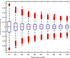
Figure 1 illustrates the distribution of cosine similarities be-tween thousands of random vectors in different dimension-ality. We generated 100,000 pairs of random vectors in each case and calculated their cosine similarity and plotted the distribution of similarities with respect to the dimensionality
10 20 30 40 50 60 70 80 90 100
Dimensionality -1
-0.8 -0.6 -0.4 -0.2 0 0.2 0.4 0.6 0.8 1
Cosine Similarity
Figure 1: Distribution of cosine similarity of 100,000 pairs of random vectors. The distribution of cosine similarities is
N(0,√1
d).
of vectors. As we can see from the figure, in lower dimen-sions we have a wider distribution between [-1, +1]. But, as we increase the dimensionality, the distribution narrows down and the chances of getting two similar or dissimilar vectors is getting lower and lower. In fact, in higher dimen-sions, almost all vectors will be equidistant and almost or-thogonal to each other. Specialized distance measures have been proposed in the literature (Soleimani, Matwin, and De Souza 2015), but the curse of dimensionality in metric spaces is not well-studied.
Considering ineffectiveness of cosine similarity and every other metric in higher dimensions, we propose a kernelized variant of our objective function which improves the distri-bution of similarities and enables the algorithm to differen-tiate between the closer and further vectors.
Looking at equation (9), the repulsive force v2 consists
of a dot product of vectors in the embedded space which measures their similarity. Here, we can apply a kernel to calculate the similarities of vectors in an implicit
high-dimensional feature space. If φ(·)is the implicit mapping
function to the high-dimensional space, the kernel function
K :Rd×Rd→Rwill compute the inner product of those
vectors in an efficient way K(w~i, ~wj) = hφ(w~i), φ(w~j)i.
The gradient of the objective function is then:
∂J
∂ ~wi
=−
|V|
X
j=1
aijw~j+
|V|
X
j=1
K(w~i, ~wj)×w~j (10)
Here we apply the kernel just in the repulsive force and not in the objective function directly. PMI has proven to be able to capture the strength of association of words very well (Bullinaria and Levy 2007; Church and Hanks 1990). There-fore, we do not need to adjust the attractive force and we only want to tune the similarities in the embedded space. Moreover, applying the kernel in the repulsive force will simplify the formulation and consequently, simplify the
nu-merical optimization by preventing the derivative ofφ(.)to
appear in the gradient. Here, we propose to use a polyno-mial kernel to adjust the nonlinearity and further strengthen the effect of closer points in negative force.
K(w~i, ~wj) = (w~i. ~wj+ 1)p (11)
wherepis the degree of the polynomial kernel. Please note
dot product between [0, +1] because of the increment in the formula which makes all similarities positive. In fact, by
us-ing a polynomial kernelp≥2, the negative cosine
similar-ities are weakened while the positive cosine similarsimilar-ities are strengthened. This provides a more powerful similarity mea-sure for higher dimensions and more discriminative power for our learning algorithm.
Reducing the time complexity by approximating
the repulsive force
The most time consuming part of our algorithm is the calcu-lation of repulsive force that requires all the pairwise similar-ity calculations. Here, we propose an alternative solution and
reduce the complexity from|V|2to|V|log|V|with respect
to the size of the vocabulary. In the fast version of the
algo-rithm we only take into account theknearest neighbors of
each word for calculating the repulsive forcev2in equation
(9). This way, each wordwiattracts wordswjifaij >0(i.e.
positive PMI) and pushes away wordswjthat are among its
nearest neighborswj∈knn(wi). In fact, we do not need to
push words further away if they are already far apart, but if they are mistakenly close to the word, we use the repulsive force to improve the distribution of words. Please note that the nearest neighbors for each word are selected from the
negative set withaij = 0. This is achieved using a binary
search in the positive indices to check whether the neighbor has positive PMI or not.
We use a Vantage Point tree (VP-tree) (Yianilos 1993) combined with a heap data structure to calculate and main-tain the nearest neighbors of each word. A VP-tree is a bi-nary tree that is hierarchically built by randomly selecting a point as a vantage point and calculating the distance from the vantage point to every other point. Then using the me-dian distance as the splitting threshold, half of the points fall under the left child and the other half fall under the right child. The splitting process for each node using the median distance can be thought of centering a hyper-sphere on the vantage point in a way that half of the point are inside the hyper-sphere and the other half are outside of it.
VP-trees along withkd-trees (Toth, O’Rourke, and
Good-man 2017) and almost any other data structure suffer from the curse of dimensionality and are only suitable for low-dimensional data. In fact, in high dimensions all the points will be almost equidistant. Therefore, while searching a query point in a VP-tree, if it falls within the hypersphere of a vantage point we still need to check the outside points since the query will be very close to the median distance and the nearest neighbor may be on the other side. And sim-ilarly if the query point falls outside of the hypersphere of the vantage point we still need to check the inside points. Consequently, this leads to traversing the entire tree and its performance is no better than the exhaustive search.
There exist many approximate nearest neighbor search methods as summarized in (Muja and Lowe 2014). How-ever, due to the nature of our problem and its known struc-ture we propose our own alternative. In our algorithm, all the words are distributed on the surface of a hypersphere and therefore, their dot product is equivalent to their cosine
similarity. Cosine similarity of vectors inddimensions has
a distribution ofN(0,√1
d)(Spruill and others 2007).
Sim-ilarly, the cosine distances are distributed fromN(1,√1
d).
For instance, consideringd= 100, then the cosine distances
will be in [0.7, 1.3] range with 99.7 probability (i.e.µ±3σ).
We incorporate this information in our VP-tree search in or-der to decide whether or not the other branch needs visiting. Using this technique we get more than 99% accuracy on our
knearest neighbor search while ensuring thelog|V|search
time for each word.
By adopting the aforementioned technique, the time
com-plexity of our algorithm isO(id|V|(¯p+ (k+ log|V|) log ¯p))
wherep¯is the average number of positive examples per word
(p¯ |V|) andkis the number of nearest neighbors (i.e.
neg-ative examples) that is used.O(id|V|¯p)correspond to the
at-tractive force calculations whileO(id|V|(k+ log|V|) log ¯p)
correspond to the repulsive force calculations. log ¯p
corre-spond to the binary search inside the positive indices to en-sure that the negative set do not overlap with the positives.
KUBWE is implemented in C using the OpenMP paral-lel computing library and the source code can be found on
GitHub1.
Experiments
We have used all the articles of English Wikipedia (dump of March 2016) as the training corpus which has around 2.1 billion tokens after applying a few basic preprocessing steps. As for the vocabulary, we have limited the vocabulary to En-glish words by using the WordNet database which resulted in about 163K words. In our experiments, all the algorithms were trained on the exact same preprocessed input corpus to ensure a fair comparison. We have also used the exact same vocabulary for all the algorithms.
For the quantitative evaluation of algorithms we have used two well-known tasks of word similarity and word anal-ogy. For the word similarity task, there exist several datasets containing word pairs with their corresponding human-assigned similarity score. In this task we have used 8
dif-ferent dataset includingWordSim353(WS-ALL),WordSim
Similarity(WS-SIM) andWordSim Relatedness(WS-REL),
MEN, SimLex, MC, RG, and Stanford Rare Words (RW-STN). For the analogy task, we have used Google’s analogy dataset (Mikolov et al. 2013a) which contains 19,544
ques-tions of the form “ais toa∗asbis tob∗”. Given three of the
words, the algorithm is expected to predict the fourth word.
About half of the questions are semantic (e.g. “fatheris to
sonasmotheris todaughter”) and the other half are
syntac-tic questions (e.g. “bigis tobiggerastallis totaller”).
Analysis of the Polynomial Kernel Degree
We first analyze the effect of the kernel degree in a fixed dimensionality of 100. Our algorithm is trained using
vari-ous polynomial degrees1,3, . . . ,21and the quality of
em-beddings is measured on different word similarity and word analogy tasks. Figure 2 shows the performances with re-spect to the kernel degree. As we can see from Figures 2a
1
1 3 5 7 9 11 13 15 17 19 21 Degree of polynomial kernel 0 0.1 0.2 0.3 0.4 0.5 0.6 0.7 0.8 0.9 1
Spearman's Correlation WS353-ALL MC RG SimLex MEN RW-STANFORD Average
(a) Word similarity task
1 3 5 7 9 11 13 15 17 19 21 Degree of polynomial kernel 0.25 0.3 0.35 0.4 0.45 0.5 0.55 0.6 0.65 Accuracy Semantic Analogies Syntactic Analogies Mixed Analogies
(b) Word analogy task
Figure 2: Quality of embeddings (d = 100) obtained from
KUBWE using different kernel degrees measured on differ-ent (a) word similarity, and (b) word analogy tasks.
1 3 5 7 9 11 13 15 17 19 21
Degree of polynomial kernel 0.45 0.5 0.55 0.6 0.65 0.7 0.75 Spearman's Correlation
Dimensionality = 10 Dimensionality = 20 Dimensionality = 50 Dimensionality = 100
(a) WordSim353
1 3 5 7 9 11 13 15 17 19 21
Degree of polynomial kernel 0.55 0.6 0.65 0.7 0.75 0.8
Spearman's Correlation Dimensionality = 10 Dimensionality = 20 Dimensionality = 50 Dimensionality = 100
(b) MEN
1 3 5 7 9 11 13 15 17 19 21 Degree of polynomial kernel 0.3 0.4 0.5 0.6 0.7 0.8 0.9 Spearman's Correlation
Dimensionality = 10 Dimensionality = 20 Dimensionality = 50 Dimensionality = 100
(c) MC
Figure 3: The effect of polynomial kernel degree in differ-ent dimensionality in KUBWE algorithm evaluated on (a) WordSim353, (b) MEN, (c) MC.
and 2b the general trend is increasing as we increase the de-gree of the polynomial. This shows that in 100-dimensional space using a high degree polynomial kernel significantly improves the distribution of words, nonetheless, it reaches a plateau at some point.
In another experiment, we run the algorithm with different embedding dimensionality (10, 20, 50, and 100) and in each
case, we use various kernel degrees 1,3, . . . ,21. Figure 3
illustrates the performance of our algorithm on different di-mensionality using different kernel degrees. As we can see from the figures, generally we get better embedding as we increase the dimensionality of the embedding. This is true in other algorithms as well. We can also observe that in lower dimensions (10 and 20), using a high degree kernel will de-grade the quality of embedding significantly. This is because of distribution of cosine similarities (i.e. dot products) in the first place. If we look back at Figure 1 we see that when
d= 10andd = 20the similarities are spread all over [-1,
+1]. Using a high degree polynomial in such cases causes a few negative examples to have extremely high kernel simi-larity with the word being updated and they dominate all the rest of the negative examples. This leads to inappropriate use of negative examples which in turn deteriorates the quality of the embedding. However, in higher dimensions where the distributions of similarities are close to zero (almost orthog-onal vectors), using a higher degree polynomial will further improve the similarity calculations in the repulsive force.
Quantitative Evaluation
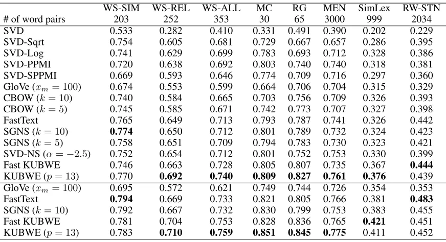
Table 1 compares 14 algorithms on 8 word similarity datasets. The numbers in the table are Pearson’s correla-tion between the rankings provided by the algorithms and the rankings of the human-scoring. These algorithms are
0.4 0.2 0.0 0.2 0.4 0.6 First principal component 0.4 0.2 0.0 0.2 0.4 0.6
Second principal component
cat dog horse rabbit fish bull lion tiger elephant frog birdcamel bear
elk leopard raccoon wolf sheep cow pig meal breakfast lunchdinner brunchsupper food cuisinesoup salt sugar stew sauce curry fruit organic spicy yummy crispy eat (a) KUBWE
2.0 1.5 1.0 0.5 0.0 0.5 1.0 1.5 2.0 First principal component 1.0 0.5 0.0 0.5 1.0 1.5 2.0
Second principal component
cat dog horse rabbit fish bulllion tigerelephant frogbird camel bearelk leopard raccoon wolf sheep cow pig meal breakfast lunch dinner brunch supper food cuisine soup salt sugar stew sauce curry fruit organic spicy yummy crispy eat (b) SGNS
Figure 4: Distribution of 40 word vectors from two groups of 20 animal names and 20 food related words. PCA algorithm is applied on 100-dimensional vectors from KUBWE (left) and SGNS (right) to obtain a 2-d visualization.
selected mainly because of their popularity and the repro-ducibility/availability of their source code. SVD, SVD-Log, and SVD-Sqrt are the factorizations of the co-occurrence, the log co-occurrence, and the square root of co-occurrence matrices, respectively. SVD-PPMI and SVD-SPPMI are the SVD factorization of the PPMI and Shifted PPMI (with shift
parameter of−log 5) matrices, respectively. SVD-NS is the
factorization of thresholded PMI table which incorporates a fraction of negative PMI values (Soleimani and Matwin 2018b). GloVe is trained with its recommended
parame-ter setting (i.e. xmax = 100). FastText is trained with the
recommended parameter settings that considers character n-grams of length 3 to 6. CBOW and SGNS are trained with negative sampling set to 5 and 10. Our proposed algorithm,
KUBWE, is trained with p = 13, and the fast KUBWE is
trained withk = 3000. The dimensionality of embeddings
is 100 in the top part of the table and 300 in the bottom 5 rows.
As we can see from Table 1, our algorithm provides the best results on 7 out of 8 datasets using 100-dimensional em-beddings and on 6 out of 8 datasets using 300-dimensional embeddings. It is noteworthy to mention that even the fast approximate version of KUBWE outperforms the state-of-the-art in 6 out of 8 word similarity tasks. Using 100-dimensional embeddings, SGNS is the best on only Word-Sim Word-Similarity dataset, and on the rest of the datasets, our method outperforms others by a good margin. We have to mention that in the analogy task GloVe provides the best results and is better than KUBWE and SGNS. However, GloVe’s performance on word similarity tasks is not com-parable with that of KUBWE and SGNS.
Qualitative Evaluation
exam-Table 1: Evaluation of different word embedding algorithms on 8 word similarity datasets. The dimensionality of the embed-dings is 100 for the top part and 300 for the bottom 5 rows. Numbers in the table are Pearson’s rank-order correlation between the human scores and scores from algorithms.
WS-SIM WS-REL WS-ALL MC RG MEN SimLex RW-STN
# of word pairs 203 252 353 30 65 3000 999 2034
SVD 0.533 0.282 0.410 0.331 0.491 0.390 0.202 0.229
SVD-Sqrt 0.754 0.605 0.681 0.729 0.667 0.657 0.286 0.395
SVD-Log 0.741 0.629 0.699 0.783 0.693 0.712 0.328 0.386
SVD-PPMI 0.720 0.638 0.692 0.803 0.740 0.740 0.318 0.381
SVD-SPPMI 0.669 0.593 0.646 0.774 0.709 0.716 0.297 0.360
GloVe (xm= 100) 0.674 0.553 0.599 0.664 0.706 0.704 0.315 0.329
CBOW (k= 10) 0.740 0.584 0.665 0.703 0.756 0.709 0.326 0.393
CBOW (k= 5) 0.745 0.585 0.671 0.742 0.773 0.707 0.327 0.398
FastText 0.765 0.649 0.713 0.793 0.787 0.741 0.326 0.442
SGNS (k= 10) 0.774 0.650 0.712 0.801 0.789 0.732 0.324 0.423
SGNS (k= 5) 0.758 0.651 0.709 0.794 0.783 0.730 0.323 0.421
SVD-NS (α=−2.5) 0.752 0.654 0.712 0.801 0.752 0.753 0.330 0.399
Fast KUBWE 0.746 0.663 0.728 0.805 0.807 0.735 0.367 0.444
KUBWE (p= 13) 0.770 0.692 0.740 0.809 0.827 0.761 0.376 0.439
GloVe (xm= 100) 0.695 0.572 0.621 0.749 0.744 0.726 0.354 0.353
FastText 0.794 0.669 0.733 0.821 0.805 0.766 0.381 0.483
SGNS (k= 10) 0.792 0.667 0.732 0.830 0.799 0.753 0.383 0.455
Fast KUBWE 0.781 0.704 0.753 0.828 0.836 0.765 0.421 0.451
KUBWE (p= 13) 0.783 0.710 0.759 0.851 0.845 0.775 0.411 0.452
0 20 40 60 80
cat dog horse rabbitbull lion tiger elephantfrog bird camelbear raccoonwolf meal breakfastlunch dinner brunch supperfood cuisinesoup stewfruit spicy yummycrispy
(a) KUBWE
0 20 40 60 80
cat dog horse rabbitbull lion tiger elephantfrog bird camelbear raccoonwolf meal breakfastlunch dinner brunch supperfood cuisinesoup stewfruit spicy yummycrispy
(b) SGNS
Figure 5: Heatmaps of 28 word vectors obtained from KUBWE (top) and SGNS (bottom). The top 14 rows in the heatmaps are animal names and the bottom 14 rows are food related words.
ples. Moreover, in the SGNS distribution “yummy” is closer to the animal group which is not correct, and “salt” and “or-ganic” are also very close to the boundary.
Figure 5 shows the heatmaps of 28 word vectors (14 an-imal names at the top and 14 food related words at the bot-tom) from the KUBWE and SGNS embeddings. In each of the heatmaps, columns are ordered by the difference be-tween the average magnitude of the features among the two word groups. Here we can see that our algorithm provides a better inter-group dissimilarity and a nicer distinction be-tween two unrelated word groups. This property will
poten-tially improve the accuracy of classifiers in many NLP tasks including text classification.
Conclusion
In this paper, we analyzed different word embedding algo-rithms and proposed our algorithm KUBWE. Our method has clear advantages over matrix factorization methods since the attractive and repulsive forces in the optimization are weighted according to the similarities in the input (i.e. smoothed PPMI) and similarities in the output (i.e. poly-nomial kernel), respectively. It has also advantages over “prediction-based” methods such as SGNS and GloVe for two main reasons: 1) The smoothed PPMI input to our al-gorithm is more reliable than the raw co-occurrence counts. 2) The adaptive way of utilizing the negative examples pre-vents the concentration effect and improves the distribution of words in the final embedding. Moreover, the effect of co-sine similarity in higher dimensions is analyzed and a ker-nelized way of calculating similarities is suggested to allevi-ate the ineffectiveness of cosine similarity. Furthermore, by adopting a modified VP-tree and approximating the repul-sive force in the optimization we reduced the computational complexity of our algorithm by orders of magnitude. Our algorithm has only one parameter which is the polynomial
degree pin the exact version and the number of negative
neighbors k in the fast approximate version. As a rule of
thumb, one should pick the degree proportionate to the log
of embedding dimensionality p ≈ logd, and the number
of negative neighbors roughly equal to the square root of the
number of words in the vocabularyk≈p
|V|. Further
References
Arora, S.; Li, Y.; Liang, Y.; Ma, T.; and Risteski, A. 2016. A latent variable model approach to pmi-based word
embed-dings. Transactions of the Association for Computational
Linguistics4:385–399.
Baroni, M., and Lenci, A. 2010. Distributional memory: A
general framework for corpus-based semantics.
Computa-tional Linguistics36(4):673–721.
Bengio, Y.; Schwenk, H.; Sen´ecal, J.-S.; Morin, F.; and
Gau-vain, J.-L. 2006. Neural Probabilistic Language Models.
Berlin, Heidelberg: Springer Berlin Heidelberg. 137–186. Bojanowski, P.; Grave, E.; Joulin, A.; and Mikolov, T. 2017.
Enriching word vectors with subword information.
Trans-actions of the Association for Computational Linguistics
5:135–146.
Bullinaria, J. A., and Levy, J. P. 2007. Extracting semantic representations from word co-occurrence statistics: A
com-putational study. Behavior research methods 39(3):510–
526.
Church, K. W., and Hanks, P. 1990. Word association norms,
mutual information, and lexicography. Computational
lin-guistics16(1):22–29.
Collobert, R., and Weston, J. 2008. A unified architecture for natural language processing: Deep neural networks with
multitask learning. InProceedings of the 25th international
conference on Machine learning, 160–167. ACM.
Deerwester, S.; Dumais, S. T.; Furnas, G. W.; Landauer, T. K.; and Harshman, R. 1990. Indexing by latent semantic
analysis. Journal of the American society for information
science41(6):391.
Joulin, A.; Grave, E.; Bojanowski, P.; and Mikolov, T. 2017.
Bag of tricks for efficient text classification. InProceedings
of the 15th Conference of the European Chapter of the Asso-ciation for Computational Linguistics, volume 2, 427–431. Lai, S.; Liu, K.; He, S.; and Zhao, J. 2016. How to generate
a good word embedding.IEEE Intelligent Systems31(6):5–
14.
Levy, O., and Goldberg, Y. 2014a. Dependency-based word
embeddings. In52nd Annual Meeting of the Association for
Computational Linguistics, volume 2, 302–308.
Levy, O., and Goldberg, Y. 2014b. Neural word
embed-ding as implicit matrix factorization. InAdvances in neural
information processing systems, 2177–2185.
Lin, C.-J. 2007. Projected gradient methods for
nonnega-tive matrix factorization. Neural computation19(10):2756–
2779.
Mikolov, T.; Chen, K.; Corrado, G.; and Dean, J. 2013a. Efficient estimation of word representations in vector space.
arXiv preprint arXiv:1301.3781.
Mikolov, T.; Sutskever, I.; Chen, K.; Corrado, G. S.; and Dean, J. 2013b. Distributed representations of words and
phrases and their compositionality. InAdvances in Neural
Information Processing Systems, 3111–3119.
Muja, M., and Lowe, D. G. 2014. Scalable nearest neighbor
algorithms for high dimensional data. IEEE transactions
on pattern analysis and machine intelligence36(11):2227– 2240.
Pantel, P., and Lin, D. 2002. Discovering word senses from
text. InProceedings of the eighth ACM SIGKDD
interna-tional conference on Knowledge discovery and data mining, 613–619. ACM.
Pennington, J.; Socher, R.; and Manning, C. D. 2014. Glove:
Global vectors for word representation. In EMNLP,
vol-ume 14, 1532–1543.
Peters, M.; Neumann, M.; Yih, W.-t.; and Zettlemoyer, L. 2018. Dissecting contextual word embeddings:
Architec-ture and representation. In Empirical Methods in Natural
Language Processing, EMNLP.
Soleimani, B. H., and Matwin, S. 2016. Nonlinear dimen-sionality reduction by unit ball embedding (ube) and its
ap-plication to image clustering. In 15th IEEE International
Conference on Machine Learning and Applications, ICMLA
2016, 983–988. IEEE.
Soleimani, B. H., and Matwin, S. 2018a. Dimensional-ity reduction and visualization by doubly kernelized unit
ball embedding. InAdvances in Artificial Intelligence: 31st
Canadian Conference on Artificial Intelligence, Canadian AI 2018, 224–230. Springer.
Soleimani, B. H., and Matwin, S. 2018b. Spectral word
embedding with negative sampling. InThirty-Second AAAI
Conference on Artificial Intelligence, AAAI 2018.
Soleimani, B. H.; Matwin, S.; and De Souza, E. N. 2015.
A density-penalized distance measure for clustering. In
Advances in Artificial Intelligence: 28th Canadian Confer-ence on Artificial IntelligConfer-ence, Canadian AI 2015, 238–249. Springer.
Spruill, M., et al. 2007. Asymptotic distribution of
coordi-nates on high dimensional spheres. Electronic
communica-tions in probability12:234–247.
Subramanian, A.; Pruthi, D.; Jhamtani, H.;
Berg-Kirkpatrick, T.; and Hovy, E. 2018. Spine: Sparse
interpretable neural embeddings. In AAAI Conference on
Aritificial Intelligence, AAAI.
Sun, F.; Guo, J.; Lan, Y.; Xu, J.; and Cheng, X. 2016. Sparse word embeddings using l1 regularized online learning. In
Proceedings of the Twenty-Fifth International Joint Confer-ence on Artificial IntelligConfer-ence, IJCAI.
Toth, C. D.; O’Rourke, J.; and Goodman, J. E. 2017.
Hand-book of discrete and computational geometry. Chapman and Hall/CRC.
Turney, P. D., and Littman, M. L. 2003. Measuring praise and criticism: Inference of semantic orientation from
asso-ciation. ACM Transactions on Information Systems (TOIS)
21(4):315–346.
Turney, P. D., and Pantel, P. 2010. From frequency to
mean-ing: Vector space models of semantics. Journal of artificial
intelligence research37:141–188.
Yianilos, P. N. 1993. Data structures and algorithms for
nearest neighbor search in general metric spaces. InSODA,