The Thirty-Third AAAI Conference on Artificial Intelligence (AAAI-19)
Spatio-Temporal Graph Routing for Skeleton-Based Action Recognition
Bin Li,
1Xi Li,
2∗Zhongfei Zhang,
1Fei Wu
21College of Information Science & Electronic Engineering, Zhejiang University, Hangzhou, China 2College of Computer Science and Technology, Zhejiang University, Hangzhou, China
{bin li, xilizju, zhongfei}@zju.edu.cn [email protected]
Abstract
With the representation effectiveness, skeleton-based human action recognition has received considerable research at-tention, and has a wide range of real applications. In this area, many existing methods typically rely on fixed physical-connectivity skeleton structure for recognition, which is in-capable of well capturing the intrinsic high-order correla-tions among skeleton joints. In this paper, we propose a novel
spatio-temporal graph routing(STGR) scheme for skeleton-based action recognition, which adaptively learns the in-trinsic high-order connectivity relationships for physically-apart skeleton joints. Specifically, the scheme is composed of two components:spatial graph router(SGR) and tempo-ral graph router(TGR). The SGR aims to discover the con-nectivity relationships among the joints based on sub-group clustering along the spatial dimension, while the TGR ex-plores the structural information by measuring the correla-tion degrees between temporal joint node trajectories. The proposed scheme is naturally and seamlessly incorporated into the framework of graph convolutional networks (GCNs) to produce a set of skeleton-joint-connectivity graphs, which are further fed into the classification networks. Moreover, an insightful analysis on receptive field of graph node is pro-vided to explain the necessity of our method. Experimental results on two benchmark datasets (NTU-RGB+D and Kinet-ics) demonstrate the effectiveness against the state-of-the-art.
Introduction
As a challenging problem in computer vision, skeleton-based human action recogntion takes 3d human body co-ordinates as input and outputs action class, which attracts increasing attention recently (Wang et al. 2018b). Typically, human body skeletons characterize the geometric body con-figuration as rigid body, and their dynamics capture mo-tion patterns in a continuous way. This dynamic geomet-ric structure expresses relation among the joints not only spatially but also temporally. By this means, graph repre-sentation is the natural way to express the intrinsic human structure. Therefore, it is crucial to automatically represent joints on the given graph. Recent success of Spatial Tem-poral Graph Convolution Networks (ST-GCN) (Yan, Xiong, and Lin 2018) has justified the effectiveness by a graph
∗
Corresponding author: Xi Li
Copyright c2019, Association for the Advancement of Artificial Intelligence (www.aaai.org). All rights reserved.
(a)
(b)
(c)
correlated
sub-group neighbour
Layer𝐿 Layer𝐿 + 1
Figure 1: Illustraion of three routing ways: (a) fixed routing by physical connections; (b) spatial routing by considering local clustering; (c) temporal routing by modeling the corre-lation degrees of node trajectories.
aggregation scheme with physical human skeleton, against the existing literatures such as pseduo images (Wang et al. 2018a; Xie et al. 2018), variants of LSTM (Shahroudy et al. 2016; Song et al. 2017; Liu et al. 2017).
fits all”, which is possibly sub-optimal. With a fixed graph, dataflow is restricted in predefined entries, which greatly de-creases the flexibility of the model. We term this as “static routing” by analogy with Computer Networking.
In contrast, we pay much attention to seeking more flexi-ble connection scheme, which adaptively learns the intrinsic high-order connectivity among skeleton joints for specific sample, referring to “dynamic routing”. In real world scenar-ios, the dynamic skeleton itself embeds rich information that implicitly shows strong connection between two physically apart joints, e.g., two hand joints in action class “clapping”. Therefore, we formulate this dynamic routing problem as a graph topology learning problem that automatically select the most informative connections for all joints. We show that dynamic routing scheme and static routing scheme are equally important in the task.
Motivated by this observation, we formulate this problem as a joint learning problem. We first learn dynamic graph topology via position and motion of the skeleton and then apply them as a prior to the GCN recognition framework. In particular, we propose a novel Spatio-Temporal Graph Routing(STGR) scheme to model the semantic connections among the joints in a disentangled way. Rather than us-ing fixed human skeleton, two sub-networks are responsible to capture both spatial and temporal dependancies between each two nodes, serving as routers for all nodes. As shown in Figure 1, aspatial graph router(SGR) discovers the con-nectivity relationships among the joints based on sub-group clustering along the spatial dimension. A temporal graph router (TGR) explores the structural information by mea-suring the correlation degrees between temporal joint node trajectories. The spatio-temporal skeleton-joint-connectivity graphs are then fed into ST-GCN in multiple routing ways.
To explain the necessity, we further introduce “receptive field on graph” by analogy with the same term in CNNs. Re-ceptive field on graph refers to coverage range that a node can draw information from. By introducing this concept, we show that fixed human skeleton would lead to highly unbal-anced problem, which could be solved by our work.
Our contribution can be summarized as follows:
• We propose a novel spatio-temporal graph routing
scheme, which is used to exploit intrinsic high-order re-lationship among skeleton joints. The module is jointly learned with classification network and better matches the action recognition task.
• We present receptive field on graph nodes to prove that the bottleneck of previous model is unbalanced receptive field for different joints, which shows effectiveness of our spatio-temporal graph routing scheme.
Related Works
Skeleton-based Action Recognition. Traditional ap-proaches for skeleton-based action recognition mainly focus onhand-crafted featuresto capture the dynamics of joint motion, such as covariance matrix of the trajectories(Hus-sein et al. 2013), lie groups (Vemulapalli, Arrate, and Chel-lappa 2014).
With the success of the deep learning, manyCNN-based methods are proposed in an end-to-end manner.To better ultilize existed powerful structures, many efforts have been made to transform raw skeleton into pseduo image in multi-ple ways, including skepxels(Liu, Akhtar, and Mian 2017), temporal-then-spatial recalibration scheme(Xie et al. 2018), and jointwise co-occurence(Li et al. 2018a).
Recurrent Neural Networks, on the other hand, effec-tively models temporal dependency. LSTMs and GRUs are proposed to learn temporal context of sequences(Shahroudy et al. 2016; Li et al. 2017). To better handle complex spatio-temporal variation factors, attention mechanism is proposed to ensure requirement of robustness, such as key frame se-lection (Song et al. 2017) and global informative joints min-ing(Liu et al. 2017).
Graph Neural Networks. Graph neural networks (GCNs) can be roughly categorized into two streams: 1) spectral domain, which is based on the Graph Fourier Transform (GFT) (Shuman et al. 2013), performs transformation on graph basis(Bruna et al. 2014). By a parameterization of K-localized convolutions, computationally efficient and local-ized filtering has been recently achieved(Defferrard, Bres-son, and Vandergheynst 2016). To alleviate expensive cost of computing eigenvalues of Laplacian matrix, Chebyshev polynomials are introduced as a truncated expansion (Ham-mond, Vandergheynst, and Gribonval 2011). 2)spatial do-main, on the other hand, learns to aggregate each node’s neighbourhood as its new hidden representation iteratively. A first-order approximation is proposed(Kipf and Welling 2017), which succeeds in semi-supervised classification. Meanwhile, some literature(Niepert, Ahmed, and Kutzkov 2016) explores to greedly converts graph into sequence and make use of 1D convolution networks.
Recently, a few works attempt to reveal the mechanism of GCNs with either metric learning (Li et al. 2018b) or jump-ing knowledge networks (Xu et al. 2018). However, cur-rent methods are mainly focused on semi-supervised clas-sification problem. In this work, we first conduct analysis on skeleton-based action recognition with the help of receptive field on graph.
Methods
In this section, we first formulate our problem and then intro-duce our Spatio-Temporal Graph Routing (STGR) scheme by describing two sub-networks—SGR and TGR respec-tively. Later we describe the overall architecture and opti-mization. At last, we discuss receptive field on graph to fur-ther verify the necessity of STGR.
Problem Formulation
A 3D human skeleton is denoted as X = {xt
n} ∈
RCin×T×N withT frames andN joints. Each individual is represented as axyz-coordinate feature vector forn-th joint att-th time step and henceCin= 3. For further convenience,
we describe single frame skeleton asXt∈
RCin×N fort-th frame and node trajectory asXn∈RCin×T forn-th joint.
Spatial Graph Router
Temporal Graph Router
Concat Graph
Convolution
Global Average Pooling
FC
Framewise skeleton
Node trajectory
Classification
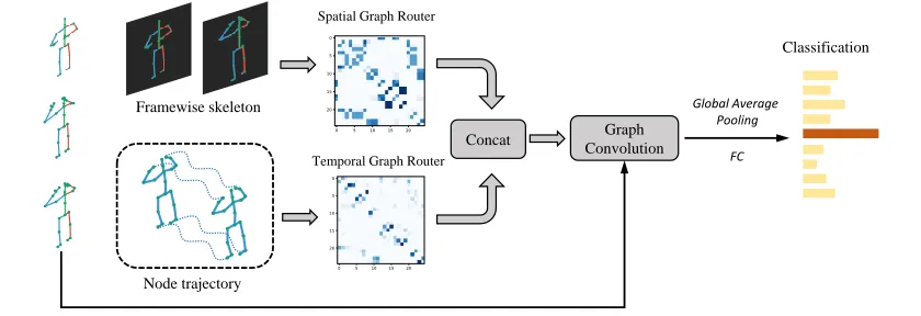
Figure 2:Overview of spatio-temporal graph router. The input 3d-skeleton sequence is first transformed as framewise skele-ton and node trajectories respectively. Then Spatial Graph Router (SGR) and Temporal Graph Router (TGR) produce new skeleton-joint-connectivity graphs respectively. ST-GCN receives this graphs and outputs action class.
Dis the corresponding degree matrix. The default graph is denoted by:
Gdefault= ˜D−1 2A˜D˜−
1
2 (1)
whereA˜ = A+I is the generalized adjacency matrix in-cluding node itself.D˜ is the corresponding degree matrix of
˜
A. Thus,Gdefaultis the diagonal normalized matrix ofA˜. As discussed above, the fixed human skeleton is insuffi-cient to model the changeable human structure in complex scenes. Our goal is to learn the mapping from the raw skele-ton to the graph topology representation:X→ Gin multiple views such as pose and motion. Therefore we have:
Gspat,Gtemp =f
STGR X;θspat, θtemp
(2) whereGspatandGtempare spatial and temporal graph topol-ogy representation.θspatandθtemp represent corresponding parameters. Gspat and Gtemp will concatenate with default graphGdefaultto form a graph setS ={Gdefault,Gspat,Gtemp}. In the following parts, we will provide a detailed description on two sub-networks.
Spatial Graph Router Sub-network
In real world scenarios, joints usually gather in a group to ex-press a specific action. In other words, the position of each joint and the distance between pairwise joints encode the in-tensity of the relation, which is crucial to guide information flow.
Spatial Graph Pool. In order to extract spatially con-nected graph, we first use a non-parametric graph cut clus-tering method (Shi and Malik 2000) for each frame skeleton Xt ∈ RCin×N, forming K groups. As for each sub-group, we treat it as a completely connected graph, which means each two nodes are connected within the same sub-group. In this way, we define a spatially connected graph for each frametand gather all these graphs to form the “Spatial Graph Pool”:
G=G1, ...,GT (3)
where for each singleGt:
Gt ij =
1, ifiandjin the same sub-group
0, otherwise (4)
Squeeze-and-Excitation Attention. Since we have al-ready obtained a series of spatially connected graphs, our goal is to select the most informative one as representative. To this end, a frame attention scheme for jointly learning framewise importance is proposed for graph fusion.
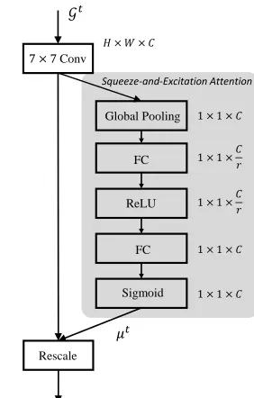
As shown in Figure 3, we model the frame attention in a Squeeze-and-Excitation way (Hu, Shen, and Sun 2018). A large7×7 convolution is first applied to aggregate lo-cal feature.Squeezeoperation is then conducted via a global average pooling layer to obtain the intermediate feature:
mint = 1 N×N
N X
i=1
N X
j=1
fConv Gt
ij (5)
wheremin = (min
1, ..., minT)denotes a collection of inter-mediate features in temporal space. Sincemin contains the complete information for the whole graph, theExcitation op-eration can model the internal dependancy across frames.
µ=Sigmoid W2·σ W1·min (6)
whereµ = (µ1, ..., µT)denotes importance score for each frame.W1 ∈ R
T
r×T andW2 ∈ RT× T
r are1×1
transfor-mation matrix.ris the dimension reduction parameter andσ is ReLU activation function. This dimensionality reduction scheme is mainly used for exploiting the relations for tem-poral dimension. We make a weighted fusion with each of its frame importanceµtto form theGspat:
Gspat= 1 T
T X
t=1
7 × 7Conv
Global Pooling
FC
ReLU
FC
Sigmoid
𝒢𝑡
1 × 1 × 𝐶 𝐻 × 𝑊 × 𝐶
1 × 1 ×𝐶 𝑟
1 × 1 ×𝐶 𝑟
1 × 1 × 𝐶
1 × 1 × 𝐶
Rescale
𝜇𝑡
Squeeze-and-Excitation Attention
Figure 3: Network structure for Spatial Graph Router (SGR).
Temporal Graph Router Sub-network
Different from SGR sub-network, TGR sub-network consid-ers the spatio-temporal graph in a global way. Based on a simple observation, joints with high correlation degrees usu-ally implies close relation. For example, in class “walking”, hands and feet are highly correlated(swing in opposite direc-tions), indicating the discriminative relation. Inspired by this idea, TGR first encodes each node trajectory with a LSTM encoder, then models relation for each pair nodes in a self-attentive way.
LSTM encoder. As discussed above, TGR first rearranges the input sequence as N independant node trajectories Xn, n = 1, ..., N, each of which is regarded as Xn ∈ RCin×T. As shown in Figure 4, a LSTM unit first encodes each input node trajectory and outputs the hidden state at the last time step:
hn,t=ψ(Xn, hn,t−1) (8)
whereψdenotes LSTM module.hn,tis the output at the last time steps.hn,tis then taken as input of the relation model-ing network to capture the interaction between two nodes. For clarity, we denotehn,tasvnfor each node.
Relation modeling. We model the pairwise node relation in the encoded feature space. Similar to rencent work (Wang et al. 2018c), we measure the relation by normalized dot product. Particularly, given each trajectory’s encoded feature v= [v1, ..., vN], The pairwise similarity is proposed as:
D(vi, vj) =θ(vi)
T
·ϕ(vj) (9)
whereθandϕare two1×1transformation operations. By performing a dot-product, we examine two nodes by their cosine distance. After computing each pairwise distance, we
LSTM Enc.
MLP: 𝜃
Softmax
Node Trajectories
𝐶 × 𝑁
MLP: 𝜑
𝐶′× 𝑁 𝐶′× 𝑁
𝑁 × 𝑁
𝒢Temp
Figure 4: Network structure for Temporal Graph Router (TGR).
further apply a softmax operation in each row, ensuring sum of all entries of a single node will be set to 1.
Gijtemp= expD(vi, vj)
PN
k=1expD(vk, vj)
(10)
Network Architecture and Optimization
In this section, we introduce the overall network architec-ture. Our model is constructed by STGR and ST-GCN. In particular, STGR is responsible to explore intrinsic connec-tivity relationships for semantically related joints in both spatial and temporal domains. ST-GCN takes both 3D skele-ton and the graph as input and output action class. In particu-lar, ST-GCN stacks multiple “GCN-TCN” units(Yan, Xiong, and Lin 2018) for representation learning, of which each “GCN-TCN” unit is seen as one layer. Each GCN unit per-forms graph convolution operation with default graphGdefault and learned graphGspatandGtempin spatial dimension while TCN unit is applied in temporal dimension to get high-level feature maps.
To make it clear, suppose hidden feature of specific node ninl-th layer is denoted byhl
v ∈Rdl. For consistency, we assumeh0=X andd0=Cin. Vanilla ST-GCN can then be
interpreted as:
hlv+1=σ M ⊗ Gdefault hlvwl
+hlv (11)
whereM represents a learnable mask to further enlarge the model’s expressive power. ⊗is element-wise product and wldenotes a regular convolution operation right after graph convolution. Along with our STGR, we produce a series of spatial and temporal graphGispat,Gitemp,i= 1, ..., Lfor each layer respectively. We do not share weights of each unit of STGR since the model is lightweight.
(b)
(a) (c)
Graph Representation
Visualization of connections
Figure 5: Comparison of 3 types of connections. (a) phys-ical connection; (b) learned spatial connection with SGR; (c) learned temporal connection with TGR. Above are ma-trix representaions of graphs. Below are the corresponding visualizations of joint connections. For better view, the con-nections are binarized with threshold 0.05 in visualizations.
hlv+1=σ X G∈S
(MG⊗ G)hlvw l G
!
+hlv (12)
whereS =
Gdefault,Gspat,Gtemp .M
G andwGl are the cor-responding mask and convolution for the specific graph. We stack multiple GCN-TCN units and then apply global av-erage pooling and full connected layer to obtain the action scoreyˆ:
ˆ
y=fST-GCN X;G spat
1 ,G
temp
1 , ...G
spat
L ,G
temp L
(13)
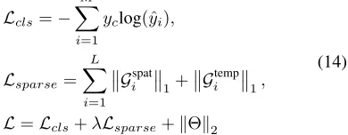
We employ standard cross-entropy loss for classification. As for the two sub-networks, to ensure the graph sparsity, the L1loss is employed:
Lcls=− M X
i=1
yclog(ˆyi),
Lsparse= L X
i=1
Gispat
1+ Gitemp
1,
L=Lcls+λLsparse+kΘk2
(14)
whereM is the overall the number of action classes,yc rep-resents the ground truth label.Θis the overall parameters for both ST-GCN and STGR.λis used to balance the weights of classification loss and sparsity loss.
Discussion
In this section, we verify the necessity of STGR in an analyt-ical way. We first introduce an intuitive definition on “recep-tive field” and then point out that “star-structure” of human skeleton makes it hard for feature sharing between two limb nodes.
(a)
(b)
Figure 6: Comparison of the receptive of torso joint (lower back) and non-torso joint (right hand). (a) Receptive field of joint “right hand”, left: after 3 steps diffusion. right: after 8 steps diffusion; (b) Receptive field of joint “lower back”. left: after 3 steps diffusion. right: after 8 steps diffusion. Red color denotes high probability, purple color denotes low probability.
Receptive field is an important notation in CNNs which reveals the spatial context for a single neuron. By analogy with this idea, we introduce the concept “receptive field on graph”, refering to the coverage range where a single node could draw information.
Figure 5 illustrates 3 types of connection mode. (a) de-notes the predefined human skeleton while (b) and (c) show the learned connections with our SGR and TGR respectively. It is straightforward that the predefined skeleton organizes itself to form a “star-structure”, in which a torso connects head and all four limbs. In this way, the centeral torso joints would spread far quicker than marginal limb joints, leading to great imbalance.
For illustration, we check the receptive field of a limb joint(right hand) and a torso joint(lower back) in Figure 6. Following previous literature(Xu et al. 2018), we cast the spreation of the Graph convolution into a k-step random walk process. The color represents the proportion of infor-mation which a node receive. As shown in Figure 6, after 3 steps diffusion, both two joints receive information from a relatively small range. After 8 steps the torso joint can nearly receive global information while the right hand joint still struggling in a small region.
Experiments
In this section we evaluate our STGR scheme in skeleton-based action recognition datasets. We conduct experiments on two large-scale datasets: NTU-RGB+D and Kinetics. We first introduce our implementation details and then perform an ablation study on various settings of the spatio-temporal graph routing scheme. Last we compare our full model with other state-of-the-art approaches. All experiments are con-ducted on 4 GTX 1080Ti GPUs.
Datasets
NTU-RGB+D. NTU-RGB+D (Shahroudy et al. 2016) is a widely used large scale skeleton-based human action recog-nition dataset. It contains 56880 skeleton sequences with 60 action classes. The overall action classes are roughly di-vided as daily action, medical condition, and mutual action. Each action is captured by cameras at the same height but from three different horizontal angles:−45◦,0◦, and45◦. Each human skeleton is represented as 3D-coordinates of 25 joints. Mutual action classes contain two subjects while the others contain only one subject. NTU-RGB+D recom-mends two evaluation protocals: 1).Cross-subject(X-Sub): The training and testing sets are divided into 40320 clips and 16560 clips respectively according to the difference of experiment subjects. 2). Cross-view (X-View): The train-ing set is collected with camera view 2 and 3 with 37920 clips, while the evaluation set is collected from camera view 1 with 18960 clips. By following the convention of existing works (Yan, Xiong, and Lin 2018) for skeleton-based action recogntion, we report the top-1 accuracy on both two proto-cals.
Kinetics. Deepmind Kinetics is recently one of the largest human action dataset. The dataset contains nearly 300,000 video clips lasts around 10 seconds. To cover as many real occasions as possible, Kinetics collects videos from YouTube, composing 400 action classes. Note that raw Ki-netics dataset contains only raw video clips. Following the previous practice (Yan, Xiong, and Lin 2018), we first ex-tract raw 2D-coordinates with the help of OpenPose toolbox (Cao et al. 2017), then apply our model. Similar to NTU-RGB+D, we extract 18 human joints and select 2 people with highest average joint confidence as main subject. In practice, we use the released data from (Yan, Xiong, and Lin 2018) to evaluate our model. The dataset is divided as train-ing set with 240,000 clips and testtrain-ing set with 20,000 clips. In this experiment, we report both top-1 and top-5 accuracy.
Implementation Details
To ease computational burden, different from previous zero padding (Yan, Xiong, and Lin 2018), we first downsample sequence length to a fixed size 64 frames, which we conduct uniform sampling with bilinear interpolation when sequence length is larger than 64 while zero padding when the given sequence is shorter than 64. In practice, we also conduct normalization for each frame, which makes training process more stable.
As for training, the whole network is trained with SGD optimizer with learning rate 0.1 for ST-GCN and 0.01 for
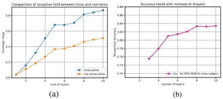
(a) (b)
Figure 7: (a) Comparison of receptive field trends for torso joints and non-torso joints with increase of number of layers; (b) Recognition accuracy trend with increase of number of layers.
STGR. The weight decay is 1e−4 and the batch size is set as 32. The balance parameterλof classification loss and L1loss is set as 0.2 since we mainly focus on classification result. We divide learning rate by 10 for both modules when monitoring validation loss stoping decrease over 5 epoches. Inspired by recent success (Li et al. 2018a) on skelteton-based action recognition, a “two-stream” scheme is applied to fuse both skeleton feature and motion feature. We need 60 training epoches for model convergence.
Ablation Study
In this section, we examine the effectivenss of our proposed STGR method and conduct experiments to test various pa-rameter settings. All experiments are conducted on X-Sub benchmark on NTU-RGB+D dataset.
Receptive field In this work, we examine the necessity of STGR. According to Figure 7(a), we first divide all 25 joints into torso joints (root, lower back, upper back) and non-torso joints (the others). Then we calculate the average receptive field from 1 layer (1-step forward) to 10 layers (which we use in model) for two set respectively. The figure shows both two sets enlarge their receptive field with more layers. However, torso joints increase with an obvious faster speed, which verifies our analysis on human skeleton structure.
Additionally, we test the vanilla ST-GCN with different number of layers. We find the recognition accuracy follows the same trend with average receptive field. As shown in Fig-ure 7(b), The accuracy increases fast initially. After 5 layers, the increasing speed becomes slow down. When approach-ing to 10 layers, the accuracy becomes stable. Stackapproach-ing more layers would not affect the overall accuracy.
When reaching certain stage, both torso and limb joints are restricted into a relatively fixed range, which limits fur-ther improvement. It would be beneficial to very deep struc-ture. However, such model brings large computational bur-den. In contrast, STGR effectively solves this problem by directly learning joint-joint connections.
# ClustersK Accuracy (%)
3 84.63
4 84.79
5 85.22
6 85.02
7 84.84
8 84.01
Table 1: Comparison of the accuracies for different number of clusters.
In theory, too many clusters usually lead to over-splitting while under-splitting is mainly caused by too few clusters. We found that the performance is generally robust with its value ranging from 3 to 7. Therefore, our choice just keeps a good balance.
Spatio-Temporal Graph Router As introduced above, the STGR is composed by two sub-networks – SGR and TGR. Table 2 shows that our proposed STGR can benefit for the vanilla ST-GCN.
Methods Accuracy (%)
Baseline (ST-GCN) 83.38
STGR-GCN (w/SGR) 85.22
STGR-GCN (w/TGR) 84.70
STGR-GCN (full) 85.80
2s-STGR-GCN (full) 86.98
Table 2: Recognition accuracies with STGR module in NTU-RGB+D X-Sub.
In this part, we examine four variants of STGR-GCN to test the effectiveness of STGR module. The four variants includes: 1) GCN with spatial graph router; 2) GCN with temporal graph router; 3) GCN with spatio-temporal graph router; 4) Two stream GCN with spatio-temporal graph router.
The proposed method improves the baseline accuracy by 1.84% and 1.32% for SGR and TGR respectively. From the results, SGR performs slightly better than TGR. With the “two stream trick”, the proposed model further improves by 1.18%, which is an effective practice in skeleton-based ac-tion recogniac-tion.
Comparison with state-of-the-art
In this section, we evaluate our full STGR-GCN model with existed state-of-the-art skeleton-based action recogni-tion models in NTU-RGB+D and Kinetics dataset.
NTU-RGB+D We roughly divide previous state-of-the-art methods into four categories: 1) Hand-crafted meth-ods: Lie group (Vemulapalli, Arrate, and Chellappa 2014); 2) RNN-based methods: STA-LSTM (Song et al. 2017), RNN-T/ACH (Li et al. 2017), GCA-LSTM (Liu et al. 2017); 3) CNN-based methods: Joint Trajectory Maps(Wang et al. 2018a), Skepxels (Liu, Akhtar, and Mian 2017), Tem-poral Conv (Kim and Reiter 2017), HCN (Li et al. 2018a); 4) Graph-based method: ST-GCN (Yan, Xiong, and Lin 2018).
Methods Accuracy (%)
X-Sub X-View
Lie group 50.1 52.8
STA-LSTM 73.4 81.2
RNN-T/ACH 74.6 83.2
GCA-LSTM 74.4 82.8
Joint Trajectory Maps 76.3 81.1
Temporal Conv 74.3 84.1
Skepxels 81.3 89.2
HCN 86.5 91.1
ST-GCN 81.5 88.3
STGR-GCN 86.9 92.3
Table 3: Recognition performance on NTU-RGB+D dataset. We compare out model with previous state-of-the-art on both crsss-subject(X-Sub) and cross-view(X-View).
Our STGR-GCN model, with simple spatio-temporal routing method, presents better results compared with vanilla ST-GCN and further achieves state-of-the-art, im-plying the effectiveness of dynamic routing scheme among graph convolution layers.
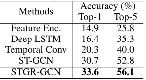
Kinetics On Kinetics, we compare our mdoel with one hand crafted approach: Feature encoding (Fernando et al. 2015); one RNN method: Deep LSTM (Shahroudy et al. 2016); a temporal-based CNN method: (Kim and Reiter 2017) and ST-GCN (Yan, Xiong, and Lin 2018). Following routine, we report both Top-1 and Top-5 accuracy.
Methods Accuracy (%)
Top-1 Top-5
Feature Enc. 14.9 25.8
Deep LSTM 16.4 35.3
Temporal Conv 20.3 40.0
ST-GCN 30.7 52.8
STGR-GCN 33.6 56.1
Table 4: Recognition performance on Kinetics dataset. We report Top-1 and Top-5 accuracy.
Conclusion
This paper presents a novel routing scheme to generate spatio-temporal related graph for physically apart joints in skeleton-based action recognition, which solves the weak-ness of predefined human structure. Furthermore, we show the importance of constructing necessary connections by in-troducing receptive field on graph, which is effectively en-larged by our work. Qualitative and quantitative results are presented to verify the effectiveness of our method.
Acknowledgements
LR19F020004, ZhiJiang Lab (2018EC0ZX01-2), the Na-tional Basic Research Program of China under Grant 2015CB352302, Zhejiang University K.P.Chao’s High Technology Development Foundation, the fundamen-tal research funds for central universities in China (2017FZA5007), Zhejiang provincial engineering research center on network media data cloud processing and analy-sis technologies, Tencent AI Lab Rhino-Bird Joint Research Program(No. JR201806), and the funding from HIKVision and ZJU Converging Media Computing Lab.
References
Bruna, J.; Zaremba, W.; Szlam, A.; and Lecun, Y. 2014. Spectral networks and locally connected networks on graphs. InInternational Conference on Learning Represen-tations (ICLR2014), CBLS, April 2014.
Cao, Z.; Simon, T.; Wei, S. E.; and Sheikh, Y. 2017. Re-altime multi-person 2d pose estimation using part affinity fields. InIEEE Conference on Computer Vision and Pattern Recognition, 1302–1310.
Defferrard, M.; Bresson, X.; and Vandergheynst, P. 2016. Convolutional neural networks on graphs with fast localized spectral filtering. InAdvances in Neural Information Pro-cessing Systems, 3844–3852.
Fernando, B.; Gavves, E.; Oramas, M. J.; Ghodrati, A.; and Tuytelaars, T. 2015. Modeling video evolution for action recognition. InComputer Vision and Pattern Recognition, 5378–5387.
Hammond, D. K.; Vandergheynst, P.; and Gribonval, R. 2011. Wavelets on graphs via spectral graph theory.Applied and Computational Harmonic Analysis30(2):129–150. Hu, J.; Shen, L.; and Sun, G. 2018. Squeeze-and-excitation networks. InThe IEEE Conference on Computer Vision and Pattern Recognition (CVPR).
Hussein, M. E.; Torki, M.; Gowayyed, M. A.; and El-Saban, M. 2013. Human action recognition using a temporal hi-erarchy of covariance descriptors on 3d joint locations. In IJCAI, volume 13, 2466–2472.
Kay, W.; Carreira, J.; Simonyan, K.; Zhang, B.; Hillier, C.; Vijayanarasimhan, S.; Viola, F.; Green, T.; Back, T.; and Natsev, P. 2017. The kinetics human action video dataset. Kim, T. S., and Reiter, A. 2017. Interpretable 3d human action analysis with temporal convolutional networks. In IEEE Conference on Computer Vision and Pattern Recogni-tion Workshops, 1623–1631.
Kipf, T. N., and Welling, M. 2017. Semi-supervised classi-fication with graph convolutional networks. InInternational Conference on Learning Representations (ICLR).
Li, W.; Wen, L.; Chang, M. C.; Lim, S. N.; and Lyu, S. 2017. Adaptive rnn tree for large-scale human action recog-nition. InIEEE International Conference on Computer Vi-sion, 1453–1461.
Li, C.; Zhong, Q.; Xie, D.; and Pu, S. 2018a. Co-occurrence feature learning from skeleton data for action recognition and detection with hierarchical aggregation. InIJCAI, 786– 792.
Li, R.; Wang, S.; Zhu, F.; and Huang, J. 2018b. Adap-tive graph convolutional neural networks. arXiv preprint arXiv:1801.03226.
Liu, J.; Akhtar, N.; and Mian, A. 2017. Skepxels: Spatio-temporal image representation of human skeleton joints for action recognition. arXiv preprint arXiv:1711.05941. Liu, J.; Wang, G.; Hu, P.; Duan, L.-Y.; and Kot, A. C. 2017. Global context-aware attention lstm networks for 3d action recognition. In The IEEE Conference on Computer Vision and Pattern Recognition (CVPR), volume 7, 43.
Niepert, M.; Ahmed, M.; and Kutzkov, K. 2016. Learning convolutional neural networks for graphs. InInternational conference on machine learning, 2014–2023.
Shahroudy, A.; Liu, J.; Ng, T.-T.; and Wang, G. 2016. Ntu rgb+ d: A large scale dataset for 3d human activity analysis. InProceedings of the IEEE conference on computer vision and pattern recognition, 1010–1019.
Shi, J., and Malik, J. 2000. ”normalized cuts and image seg-mentation”, ieee trans.IEEE Trans.pattern Anal.mach.intell 22(8):888–905.
Shuman, D. I.; Narang, S. K.; Frossard, P.; Ortega, A.; and Vandergheynst, P. 2013. The emerging field of signal pro-cessing on graphs: Extending high-dimensional data analy-sis to networks and other irregular domains. IEEE Signal Processing Magazine30(3):83–98.
Song, S.; Lan, C.; Xing, J.; Zeng, W.; and Liu, J. 2017. An end-to-end spatio-temporal attention model for human action recognition from skeleton data. InAAAI, volume 1, 4263–4270.
Vemulapalli, R.; Arrate, F.; and Chellappa, R. 2014. Human action recognition by representing 3d skeletons as points in a lie group. In IEEE Conference on Computer Vision and Pattern Recognition, 588–595.
Wang, P.; Li, W.; Li, C.; and Hou, Y. 2018a. Action recogni-tion based on joint trajectory maps with convolurecogni-tional neural networks. Knowledge-Based Systems.
Wang, P.; Li, W.; Ogunbona, P.; Wan, J.; and Escalera, S. 2018b. Rgb-d-based human motion recognition with deep learning: A survey. Computer Vision and Image Under-standing.
Wang, X.; Girshick, R.; Gupta, A.; and He, K. 2018c. Non-local neural networks. In The IEEE Conference on Com-puter Vision and Pattern Recognition (CVPR).
Xie, C.; Li, C.; Zhang, B.; Chen, C.; Han, J.; and Liu, J. 2018. Memory attention networks for skeleton-based action recognition. InIJCAI, 1639–1645.
Xu, K.; Li, C.; Tian, Y.; Sonobe, T.; Kawarabayashi, K.-i.; and Jegelka, S. 2018. Representation learning on graphs with jumping knowledge networks. arXiv preprint arXiv:1806.03536.