Unsupervised Basis Function Adaptation
for Reinforcement Learning
Edward Barker [email protected]
School of Mathematics and Statistics University of Melbourne
Melbourne, Victoria 3010, Australia
Charl Ras [email protected]
School of Mathematics and Statistics University of Melbourne
Melbourne, Victoria 3010, Australia
Editor:George Konidaris
Abstract
When using reinforcement learning (RL) algorithms it is common, given a large state space, to introduce some form of approximation architecture for the value function (VF). The exact form of this architecture can have a significant effect on an agent’s performance, however, and determining a suitable approximation architecture can often be a highly complex task. Consequently there is currently interest among researchers in the potential for allowing RL algorithms to adaptively generate (i.e. to learn) approximation architectures. One rela-tively unexplored method of adapting approximation architectures involves using feedback regarding the frequency with which an agent has visited certain states to guide which areas of the state space to approximate with greater detail. In this article we will: (a) informally discuss the potential advantages offered by such methods; (b) introduce a new algorithm based on such methods which adapts a state aggregation approximation architecture on-line and is designed for use in conjunction with SARSA; (c) provide theoretical results, in a policy evaluation setting, regarding this particular algorithm’s complexity, convergence properties and potential to reduce VF error; and finally (d) test experimentally the extent to which this algorithm can improve performance given a number of different test problems. Taken together our results suggest that our algorithm (and potentially such methods more generally) can provide a versatile and computationally lightweight means of significantly boosting RL performance given suitable conditions which are commonly encountered in practice.
Keywords: reinforcement learning, unsupervised learning, basis function adaptation, state aggregation, SARSA
1. Introduction
Traditional reinforcement learning (RL) algorithms such as TD(λ) (Sutton, 1988) or Q-learning (Watkins and Dayan, 1992) can generate optimal policies, when dealing with small state and action spaces, by exactly representing the value function (VF). However, when
c
environments are complex (with large or continuous state or action spaces), using such algorithms directly becomes too computationally demanding. As a result it is common to introduce some form of architecture with which to approximate the VF, for example a parametrised set of functions (Sutton and Barto, 2018; Bertsekas and Tsitsiklis, 1996). One issue when introducing VF approximation, however, is that the accuracy of the algorithm’s VF estimate, and as a consequence its performance, is highly dependent upon the exact form of the architecture chosen (it may be, for example, that no element of the chosen set of parametrised functions closely fits the VF). Accordingly, a number of authors have explored the possibility of allowing the approximation architecture to belearned by the agent, rather than pre-set manually by the designer—see Busoniu et al. (2010) for an overview. It is hoped that, by doing this, we can design algorithms which will perform well within a more general class of environment whilst requiring less explicit input from designers.1
A simple and perhaps, as yet, under-explored method of adapting an approximation architecture involves using an estimate of the frequency with which an agent has visited certain states to determine which states should have their values approximated in greater detail. We might be interested in such methods since, intuitively, we would suspect that areas which are visited more regularly are, for a number of reasons, more “important” in relation to determining a policy. Such a method can be contrasted with the more commonly explored method of explicitly measuring VF error and using this error as feedback to adapt an approximation architecture. We will refer to methods which adapt approximation archi-tectures using visit frequency estimates as being unsupervised in the sense that no direct reference is made to reward or to any estimate of the VF.
Our intention in this article is to provide—in the setting of problems with large or continuous state spaces, where reward and transition functions are unknown, and where our task is to maximise reward—an exploration of unsupervised methods along with a discussion of their potential merits and drawbacks. We will do this primarily by introducing an algorithm, PASA, which represents an attempt to implement an unsupervised method in a manner which is as simple and obvious as possible. The algorithm will form the principle focus of our theoretical and experimental analysis.
It will turn out that unsupervised techniques have a number of advantages which may not be offered by other more commonly used methods of adapting approximation architec-tures. In particular, we will argue that unsupervised methods have (a) low computational overheads and (b) a tendency to require less sampling in order to converge. We will also argue that the methods can, under suitable conditions, (c) decrease VF error, in some cases significantly, with minimal input from the designer, and, as a consequence, (d) boost perfor-mance. The methods will be most effective in environments which satisfy certain conditions, however these conditions are likely to be satisfied by many of the environments we encounter most commonly in practice. We will also see that the principle of using state visit frequency can, perhaps counter-intuitively, interact favourably with the process of exploration.2 The 1. Introducing the ability to adapt an approximation architecture is in some ways similar to simply adding additional parameters to an approximation architecture. However separating parameters into two sets, those adjusted by the underlying RL algorithm, and those adjusted by the adaptation method, permits us scope to, amongst other things, specify two distinct update rules.
fact that unsupervised methods are cheap and simple, yet still have significant potential to enhance performance, makes them appear a promising, if perhaps somewhat overlooked, means of adapting approximation architectures.
1.1. Article Overview
Our article is structured as follows. Following some short introductory sections we will offer an informal discussion of the potential merits of unsupervised methods in order to motivate and give a rationale for our exploration (Section 1.5). We will then propose (in Section 2) our new algorithm, PASA, short for “Probabilistic Adaptive State Aggregation”. The algorithm is designed to be used in conjunction with SARSA, and adapts a state aggregation approximation architecture on-line.
Section 3 is devoted to a theoretical analysis of the properties of PASA. Sections 3.1 to 3.3 relate to finite state spaces. We will demonstrate in Section 3.1 that PASA has a time complexity (considered as a function of the state and action space sizes, S and A) of the same order as its SARSA counterpart, i.e. O(1). It has space complexity of O(X) as a function of S, where X is the number of cells in the state aggregation architecture, and O(1) as a function of A. This is compared to O(X) andO(A) respectively for its SARSA counterpart. This means that PASA is computationally cheap: it does not carry significant computational cost beyond SARSA with fixed state aggregation.
In Section 3.2 we investigate PASA in the context of where an agent’s policy is held fixed and prove that the algorithm converges. This implies that, unlike non-linear architectures in general, SARSA combined with PASA will have the same convergence properties as SARSA with a fixed linear approximation architecture (i.e. the VF estimate may, assuming the policy is updated, “chatter”, or fail to converge, but will never diverge).
In Section 3.3 we will use PASA’s convergence properties to obtain a theorem, again where the policy is held fixed, regarding the impact PASA will have on VF error. This theorem guarantees that VF error will be arbitrarily low as measured by routinely used scoring functions provided certain conditions are met, conditions which require primarily that the agent spends a large amount of the time in a small subset of the state space. This result permits us to argue informally that PASA will also, assuming the policy is updated, improve performance given similar conditions.
In Section 3.4 we extend the finite state space concepts to continuous state spaces. We will demonstrate that, assuming we employ an initial arbitrarily complex discrete approxi-mation of the agent’s continuous input, all of our discrete case results have a straightforward continuous state space analogue, such that PASA can be used to reduce VF error (at low computational cost) in a manner substantially equivalent to the discrete case.
and policy are sufficiently close to deterministic and the algorithm has X =X(S) ≥f(S) cells available in its adaptive state aggregation architecture, where f is O(√SlnSlog2S).
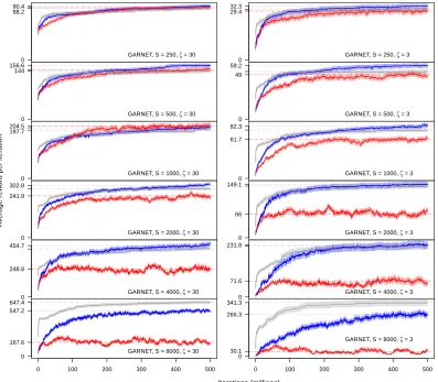
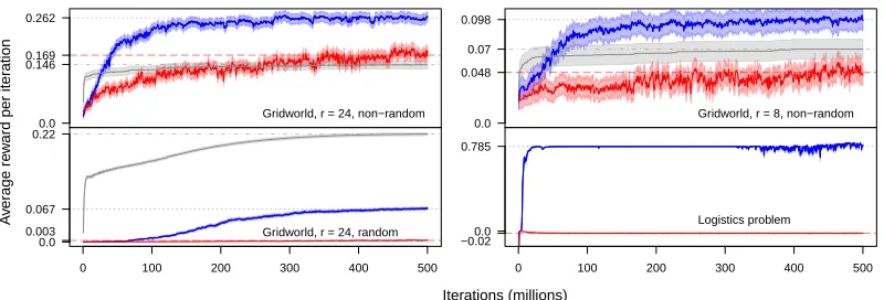
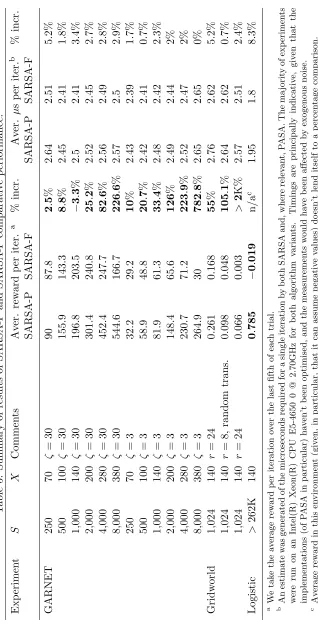
To corroborate our theoretical analysis, and to further address the more complex ques-tion of whether PASA will improve overall performance, we outline some experimental results in Section 4. We explore three different types of environment: a GARNET environ-ment,3 a “Gridworld” type environment, and an environment representative of a logistics problem.
Our experimental results suggest that PASA, and potentially, by extension, techniques based on similar principles, can significantly boost performance when compared to SARSA with fixed state aggregation. The addition of PASA improved performance in all but one of our experiments,4 and regularly doubled or even tripled the average reward obtained. Indeed, in some of the environments we tested, PASA was also able to outperform SARSA with no state abstraction, the potential reasons for which we discuss in Section 4. This is despite minimal input from the designer with respect to tailoring the algorithm to each distinct environment type.5 Furthermore, in each case the additional processing time and resources required by PASA are measured and shown to be minimal, as predicted.
1.2. Related Works
The concept of using visit frequencies in an unsupervised manner is not completely new however it remains relatively unexplored compared to methods which seek to measure the error in the VF estimate explicitly and to then use this error as feedback. We are aware of only three papers in the literature which investigate a method similar in concept to the one that we propose, though the algorithms analysed in these three papers differ from PASA in some key respects.
Moreover there has been little by way of theoretical analysis of unsupervised techniques. The results we derive in relation to the PASA algorithm are all original, and we are not aware of any published theoretical analysis which is closely comparable.
In the first of the three papers just mentioned, Menache et al. (2005) provide a brief evaluation of an unsupervised algorithm which uses the frequency with which an agent has visited certain states to fit the centroid and scale parameters of a set of Gaussian basis functions. Their study was limited to an experimental analysis, and to the setting of policy evaluation. The unsupervised algorithm was not the main focus of their paper, but rather was used to provide a comparison with two more complex adaptation algorithms which used information regarding the VF as feedback.6
In the second paper, Nouri and Littman (2009) examined using a regression tree approx-imation architecture to approximate the VF for continuous multi-dimensional state spaces. Each node in the regression tree represents a unique and disjoint subset of the state space.
3. An environment with a discrete state space where the transition function is deterministic and generated uniformly at random. For more details refer to Sections 3.5 and 4.1.
4. The single exception was likely to have been affected by experimental noise. See Section 4.1.
5. For each problem, with the exception of the number of cells available to the state aggregation architecture, the PASA parameters were left unchanged
Once a particular node has been visited a fixed number of times, the subset it represents is split (“once-and-for-all”) along one of its dimensions, thereby creating two new tree nodes. The manner in which the VF estimate is updated7 is such that incentive is given to the agent to visit areas of the state space which are relatively unexplored. The most important differences between their algorithm and ours are that, in their algorithm, (a) cell-splits are permanent, i.e. once new cells are created, they are never re-merged and (b) a permanent record is kept of each state visited (this helps the algorithm to calculate the number of times newly created cells have already been visited). With reference to (a), the capacity of PASA to re-adapt is, in practice, one of its critical elements (see Section 3). With reference to (b), the fact that PASA does not retain such information has important implications for its space complexity. The paper also provides theoretical results in relation to the optimality of their algorithm. Their guarantees apply in the limit of arbitrarily precise VF representa-tion, and are restricted to model-based settings. In these and other aspects their analysis differs significantly from our own.
In the third paper, which is somewhat similar in approach and spirit to the second (and which also considers continuous state spaces), Bernstein and Shimkin (2010) examined an algorithm wherein a set of kernels are progressively split (again “once-and-for-all”) based on the visit frequency for each kernel. Their algorithm also incorporates knowledge of uncertainty in the VF estimate, to encourage exploration. The same two differences to PASA (a) and (b) listed in the paragraph above also apply to this algorithm. Another key difference is that their algorithm maintains a distinct set of kernels for each action, which implies increased algorithm space complexity. The authors provide a theoretical analysis in which they establish a linear relationship between policy-mistake count8 and maximum cell size in an approximation of the VF in a continuous state space.9 The results they provide are akin to other PAC (“probably approximately correct”) analyses undertaken by several authors under a range of varying assumptions—see, for example, Strehl et al. (2009) or, more recently, Jin et al. (2018). Their theoretical analysis differs from ours in many fundamental respects. Unlike our theoretical results in Section 3, their results have the advantage that they are not dependent upon characteristics of the environment and pertain to performance, not just VF error. However, similar to Nouri and Littman (2009) above, they carry the significant limitation that there is no guarantee of arbitrarily low policy-mistake count in the absence of an arbitrarily precise approximation architecture, which is equivalent in this context to arbitrarily large computational resources.10
There is a much larger body of work less directly related to this article, but which has central features in common, and is therefore worth mentioning briefly. Two important threads of research can be identified.
First, as noted above, a number of researchers have investigated the learning of an approximation architecture using feedback regarding the VF estimate. Early work in this area includes Singh et al. (1995), Moore and Atkeson (1995) and Reynolds (2000). Such approaches most commonly involve either (a) progressively adding features
“once-and-for-7. The paper proposes more than one algorithm. We refer here to the fittedQ-iteration algorithm. 8. Defined, in essence, as the number of time steps in which the algorithm executes a non-optimal policy. 9. See, in particular, their Theorems 4 and 5.
all”—see for example Munos and Moore (2002),11 Keller et al. (2006) or Whiteson et al. (2007)—based on a criteria related to VF error, or (b) the progressive adjustment of a fixed set of basis functions using, most commonly, a form of gradient descent—see, for example, Yu and Bertsekas (2009), Di Castro and Mannor (2010) and Mahadevan et al. (2013).12 Approaches which use VF feedback form an interesting array of alternatives for adaptively generating an approximation architecture, however such approaches can be considered as “taxonomically distinct” from the unsupervised methods we are investigating. The implications of using VF feedback compared to unsupervised adaptation, including some of the comparative advantages and disadvantages, are explored in more detail in our motivational discussion in Section 1.5. We will make the argument that unsupervised methods have certain advantages not available to techniques which use VF feedback in general.
Second, given that the PASA algorithm functions by updating a state aggregation ar-chitecture, it is worth noting that a number of principally theoretical works exist in relation to state aggregation methods. These works typically address the question of how states in a Markov decision process (MDP) can be aggregated, usually based on “closeness” of the transition and reward function for groups of states, such that the MDP can be solved efficiently. Examples of papers on this topic include Hutter (2016) and Abel et al. (2016) (the results of the former apply with generality beyond just MDPs). Notwithstanding be-ing focussed on the question of how to create effective state aggregation approximation architectures, these works differ fundamentally from ours in terms of their assumptions and overall objective. Though there are exceptions—see, for example, Ortner (2013)13—the results typically assume knowledge of the MDP (i.e. the environment) whereas our work assumes no such knowledge. Moreover the techniques analysed often use the VF, or a VF estimate, to generate a state aggregation, which is contrary to the unsupervised nature of the approaches we are investigating.
It is worth, before concluding our discussion of related works, making brief mention of approaches which use gradient descent to optimise a fixed set of parameters of a complex and differentiable non-linear VF approximator.14 Such approaches encompass (in part) what are known as deep RL methods, which have recently shown impressive results on an array of challenging problems (Mnih et al., 2015; Silver et al., 2018). When using this type of approach, additional techniques are often employed to encourage stability, since few convergence guarantees exist for non-linear VF approximation architectures in general. Our algorithm, PASA, is not incompatible with these types of approach fundamentally (the SARSA algorithm which PASA supports could, hypothetically, be replaced by a non-linearly parametrised RL algorithm). However the principles underlying unsupervised basis
11. The authors in this article investigate several distinct adaptation, or “splitting”, criteria. However all depend in some way on an estimate of the value function.
12. Whilst less common, some approaches have been proposed, such as Bonarini et al. (2006), which fall somewhere in between (a) and (b). In the paper just cited the authors propose a method which involves employing a cell splitting rule offset by a cell merging (or pruning) rule.
13. This paper explores the possibility of aggregating states based on learned estimates of the transition and reward function, and as such the techniques it explores differ quite significantly from those we are investigating.
function adaptation are very different from those underlying, for example, deep RL. The motivational discussion in Section 1.5 is helpful in drawing out the core differences between unsupervised methods and approaches, such as deep RL, which apply gradient descent in conjunction with a fixed, non-linear VF approximation architecture.
1.3. Formal Framework15
We assume that we have an agent which interacts with an environment over a sequence of iterations t ∈N. We will assume throughout this article (with the exception of Section 3.4) that we have a finite set S of states of size S (Section 3.4 relates to continuous state spaces and contains its own formal definitions where required). We also assume we have a discrete set A of actions of size A. Since S and A are finite, we can, using arbitrarily assigned indices, label each statesi (1≤i≤S) and each action aj (1≤j≤A).
For each tthe agent will be in a particular state and will take a particular action. Each action is taken according to apolicy π whereby the probability the agent takes actionaj in
statesi is denoted as π(aj|si).
The transition function P:S × A × S →[0,1] defines how the agent’s state evolves over
time. If the agent is in state si and takes an action aj in iteration t, then the probability
it will transition to the state si0 in iteration t+ 1 is given by P(si0|si, aj). The transition
function must be constrained such that PSi0=1P(si0|si, aj) = 1.
Denote asRthe space of all probability distributions defined on the real line. Thereward
function R:S × A → R is a mapping from each state-action pair (si, aj) to a real-valued
random variable R(si, aj), where each R(si, aj) is defined by a cumulative distribution
function FR(si, aj) : R→ [0,1], such that if the agent is in statesi and takes action aj in
iteration t, then it will receive a real-valued reward in iterationt distributed according to R(si, aj). Some of our key results will require that |R(si, aj)| ≤ c, where c is a constant
such that 0 ≤ c < ∞, for all i and j, in which case we use Rm to denote the maximum magnitude of the expected value of R(si, aj) over all iandj.
Prior to the point at which an agent begins interacting with an environment, both P and R are taken as being unknown. However we may assume in general that we are given a prior distribution for both. Our overarching objective is to design an algorithm to adjust π during the course of the agent’s interaction with its environment so that total reward is maximised over some interval (for example, in the case of our experiments in Section 4, this will be a finite interval towards the end of each trial).
1.4. Scoring Functions
Whilst our overarching objective is to maximise performance, an important step towards achieving this objective involves reducing error in an algorithm’s VF estimate. This is based on the assumption that more accurate VF estimates will lead to better directed policy updates, and therefore better performance. A large part of our theoretical analysis in Section 3 will be directed at assessing the extent to which VF error will be reduced under different circumstances.
Error in a VF estimate for a fixed policyπis typically measured using ascoring function. It is possible to define many different types of scoring function, and in this section we will describe some of the most commonly used types.16 We first need a definition of the VF itself. We formally define thevalue function Qπγ for a particular policyπ, which maps each of the S×A state-action pairs to a real value, as follows:
Qπγ(si, aj) := E
∞
X
t=1
γt−1R s(t), a(t)
s(1)=si, a(1) =aj !
,
where the expectation is taken over the distributions of P, R and π (i.e. for particular instances ofP and R, not over their prior distributions) and where γ ∈[0,1) is known as a
discount factor. We will generally omit the subscriptγ. We have used superscript brackets
to indicate dependency on the iterationt. Initially the VF is unknown.
Suppose that ˆQ is an estimate of the VF. One commonly used scoring function is the squared error in the VF estimate for each state-action, weighted by some arbitrary function wwhich satisfies 0≤w(si, aj)≤1 for alliandj. We will refer to this as themean squared
error (MSE):
MSEγ := S X
i=1
A X
j=1
w(si, aj)
Qπγ(si, aj)−Q(sˆ i, aj) 2
. (1)
Note that the true VF Qπγ, which is unknown, appears in (1). Many approximation architecture adaptation algorithms use a scoring function as a form of feedback to help guide how the approximation architecture should be updated. In such cases it is important that the score is something which can be measured by the algorithm. In that spirit, another commonly used scoring function (which, unlike MSE, is not a function ofQπγ) usesTγπ, the
Bellman operator, to obtain an approximation of the MSE. This scoring function we denote
asL. It is a weighted sum of theBellman error at each state-action:17
Lγ := S X
i=1
A X
j=1
w(si, aj)
TγπQ(sˆ i, aj)−Q(sˆ i, aj) 2
,
where:
TγπQ(sˆ i, aj) := E (R(si, aj)) +γ S X
i0=1
P(si0|si, aj) A X
j0=1
π(aj0|si0) ˆQ(si0, aj0).
The valueLstill relies on an expectation within the squared term, and hence there may still be challenges estimating L empirically. A third alternative scoring function ˜L, which
16. Sutton and Barto (2018) provide a detailed discussion of different methods of scoring VF estimates. See, in particular, Chapters 9 and 11.
steps around this problem, can be defined as follows (FR is defined in Section 1.3):
˜ Lγ :=
S X
i=1
A X
j=1
w(si, aj) S X
i0=1
P(si0|si, aj) A X
j0=1
π(aj0|si0)
× Z
R
R(si, aj) +γQ(sˆ i0, aj0)−Q(sˆ i, aj) 2
dFR(si, aj).
These three different scoring functions are arguably the most commonly used scoring functions, and we will state results in Section 3 in relation to all three. Scoring functions which involve a projection onto the space of possible VF estimates are also commonly used. We will not consider such scoring functions explicitly, however our results below will apply to these scoring functions, since, for the architectures we consider, scoring functions with and without a projection are equivalent.
We will need to consider some special cases of the weighting function w. Towards that end we define what we will term the stable state probability vector ψ =ψ(π, s(1)), of dimensionS, as follows:
ψi:= lim
T→∞
1 T
T X
t=1
I{s(t)=s
i},
whereI is the indicator function for a logical statement such that IA= 1 if Ais true. The
value of the vectorψrepresents the proportion of the time the agent will spend in each state as t→ ∞ provided it follows the fixed policy π. In particular ψi indicates the proportion
of the time the agent spends in the state si. As implied by its definition, ψ is a function
of the policy π and the agent’s starting state s(1) (i.e. its state at t = 1). In the case where a transition matrix obtained from π and P is irreducible and aperiodic, ψ will be the stationary distribution associated withπ. None of the results in this paper relating to finite state spaces require that a transition matrix obtained from π and P be irreducible, however in order to avoid possible ambiguity, we will assume unless otherwise stated that ψ, whenever referred to, is the same for all s(1).
Perhaps the most natural, and also most commonly used, weighting coefficientw(si, aj)
is ψ(si)π(aj|si), such that each error term is weighted in proportion to how frequently the
particular state-action occurs (Menache et al., 2005; Yu and Bertsekas, 2009; Di Castro and Mannor, 2010). A slightly more general set of weightings is made up of those which satisfy w(si, aj) =ψiw(s˜ i, aj), where 0≤w(s˜ i, aj)≤1 and
PA
j0=1w(s˜ i, aj0)≤1 for all iandj. All
of our theoretical results will require thatw(si, aj) =ψiw(s˜ i, aj), and some will also require
that ˜w(si, aj) =π(aj|si).18
1.5. A Motivating Discussion
The principle we are exploring in this article is that frequently visited states should have their values approximated with greater precision. Why would we employ such a strategy? There is a natural intuition which says that states which the agent is visiting frequently are
18. It is worth noting that weighting byψandπis not necessarily the only valid choice forw. It would be possible, for example, to setw(si, aj) = 1 for alliandjdepending on the purpose for which the scoring
more important, either because they are intrinsically more prevalent in the environment, or because the agent is behaving in a way that makes them more prevalent, and should therefore be more accurately represented.
However it may be possible to pinpoint reasons related to efficient algorithm design which might make us particularly interested in such approaches. The thinking behind unsupervised approaches from this perspective can be summarised (informally) in the set of points which we now outline. Our arguments are based principally around the objective of minimising VF error (we will focus our arguments on MSE, though similar points could be made in relation toLor ˜L). We will note at the end of this section, however, circumstances under which the arguments will potentially translate to benefits where policies are updated as well.
It will be critical to our arguments that the scoring function is weighted by ψ. Accord-ingly we begin by assuming that, in measuring VF error using MSE, we adoptw(si, aj) =
ψiw(s˜ i, aj), where ˜w(si, aj) obeys the constraints noted in the previous subsection, is stored
by the algorithm, and is not a function of the environment (for example, ˜w(si, aj) =π(aj|si)
or ˜w(si, aj) = 1/Afor all iand j). Now consider:
1. Our goal is to find an architecture which will permit us to generate a VF estimate with low error. We can see, referring to equation (1), that we have a sum of terms of the form:
ψiw(s˜ i, aj)
Qπ(si, aj)−Q(sˆ i, aj) 2
.
Suppose ˆQMSE represents the value of ˆQ for which MSE is minimised subject to the constraints of a particular architecture. Assuming we can obtain a VF estimate
ˆ
Q= ˆQMSE (e.g. using a standard RL algorithm), each term in equation (1) will be of the form:
ψiw(s˜ i, aj)
Qπ(si, aj)−QMSE(sˆ i, aj) 2
.
In order to reduce MSE we will want to focus on ensuring that our architecture avoids the occurrence of large terms of this form. A term may be large either because ψi is large, because ˜w(si, aj) is large, or because Qπ(si, aj)−QˆMSE(si, aj) has large
magnitude. It is likely that any adaptation method we propose will involve directly or indirectly sampling one or more of these quantities in order to generate an estimate which can then be provided as feedback to update the architecture. Since ˜w(si, aj) is
assumed to be already stored by the algorithm, we focus our attention on the other two factors.
2. Whilst bothψandQπ−QMSEˆ influence the size of each term, in a range of important circumstances generating an accurate estimate of ψ will be easier and cheaper than generating an accurate estimate ofQπ−QˆMSE. We would argue this for three reasons: (a) An estimate ofQπ−QˆMSE can only be generated with accuracy once an accurate estimate of ˆQMSE exists. The latter will typically be generated by the underlying RL algorithm, and may require a substantial amount of training time to generate, particularly if γ is close to one;19
19. Whilst the underlying RL algorithm will store an estimate ˆQ ofQπ, having an estimate ofQπ is not the same as having an estimate of Qπ−Qˆ. If we want to estimate Qπ− ˆ
(b) The valueQπ(si, aj)−QˆMSE(si, aj) mayalso depend on trajectories followed by
the agent consisting of many states and actions (again particularly if γ is near one), and it may take many sample trajectories and therefore a long training time to obtain a good estimate, even once ˆQMSE is known;
(c) For each single value ψi there are A terms containing distinct values for Qπ−
ˆ
QMSE in the MSE. This suggests thatψ can be more quickly estimated in cases where ˜w(si, aj)>0 for more than one indexj. Furthermore, the space required
to store an estimate, if required, is reduced by a factor ofA.
3. If we accept that it is easier and quicker to estimateψ than Qπ−QMSE, we need toˆ ask whether measuring the former and not the latter will provide us with sufficient information in order to make helpful adjustments to the approximation architecture. If ψi is roughly the same value for all 1 ≤i ≤S, then our approach may not work.
However in practice there are many environments which (in some cases subject to the policy) are such that there will be a large amount of variance in the terms ofψ, with the implication that ψ can provide critical feedback with respect to reducing MSE. This will be illustrated most clearly through examples in Section 3.5.
4. Finally, from a practical, implementation-oriented perspective we note that, for fixed π, the valueQπ−QˆMSE is a function of the approximation architecture. This is not the case forψ. If we determine our approximation architecture with reference toQπ−
ˆ
QMSE, we may find it more difficult to ensure our adaptation method converges.20 This could force us, for example, to employ a form of gradient descent (thereby, amongst other things,21 limiting us to architectures expressible via differential parameters, and forcing architecture changes to occur gradually) or to make “once-and-for-all” changes to the approximation architecture (removing any subsequent capacity for our architecture to adapt, which is critical if we expect, under more general settings, the policyπ to change with time).22
To summarise, there is the possibility that in many important instances visit probability loses little compared to other metrics when assessing the importance of an area of the VF, and the simplicity of unsupervised methods allows for fast calculation and flexible implementation.
The above points focus on the problem of policy evaluation. All of our arguments will extend, however, to the policy learning setting, provided that our third point above consistently holds as each update is made. Whether this is the case will depend primarily on
in general as being estimated from scratch. The distinction is explored, for example, from a gradient descent perspective in Baird (1995). See also Chapter 11 in Sutton and Barto (2018).
20. This is because we are likely to adjust the approximation architecture so that the approximation ar-chitecture is capable of more precision for state-action pairs where Qπ(si, aj)−QˆMSE(si, aj) is large.
But, in doing this, we will presumably remove precision from other state-action pairs, resulting in
Qπ(si, aj)−QˆMSE(si, aj) increasing for these pairs, which could then result in us re-adjusting the
archi-tecture to give more precision to these pairs. This could create cyclical behaviour.
21. Gradient descent using the Bellman error is also known to be slow to converge and may require additional computational resources (Baird, 1995).
the type of environment with which the agent is interacting. This will be explored further in Section 3.5 and Section 4.
Having now discussed, albeit informally, some of the potential advantages of unsuper-vised approaches to adapting approximation architectures, we would now like to implement the ideas in an algorithm. This will let us test the ideas theoretically and empirically in a more precise, rigorous setting.
2. The PASA Algorithm
Our Probabilistic Adaptive State Aggregation (PASA) algorithm is designed to work in conjunction with SARSA (though certainly there may be potential to use it alongside other, similar, RL algorithms). In effect PASA provides a means of allowing a state aggregation approximation architecture to be adapted on-line. In order to describe in detail how the algorithm functions it will be helpful to initially provide a brief review of SARSA, and introduce some terminology relating to state aggregation approximation architectures.
2.1. SARSA with Fixed State Aggregation
In itstabular form SARSA23stores an S×Aarray ˆQ(si, aj). It performs an update to this
array in each iteration as follows:
ˆ
Q(t+1) s(t), a(t)= ˆQ(t) s(t), a(t)+ ∆ ˆQ(t) s(t), a(t), where:24
∆ ˆQ(t) s(t), a(t)=η
R s(t), a(t)+γQˆ(t) s(t+1), a(t+1)−Qˆ(t) s(t), a(t)
(2)
and where η is a fixed step size parameter.25 In the tabular case, SARSA has some well known and helpful convergence properties (Bertsekas and Tsitsiklis, 1996).
It is possible to use different types of approximation architecture in conjunction with SARSA. Parametrised value function approximation involves generating an approximation of the VF using a parametrised set of functions. The approximate VF is denoted as ˆQθ,
and, assuming we are approximating over the state space only and not the action space, this function is parametrised by a matrix of weights θ of dimension X ×A (where, by assumption,X S). Such an approximation architecture is linear if ˆQθ can be expressed
in the form ˆQθ(si, aj) =ϕ(si, aj)Tθj, whereθj is thejth column ofθandϕ(si, aj) is a fixed
vector of dimensionX for each pair (si, aj). TheXA distinct vectors of dimensionS given
by (ϕ(s1, aj)k, ϕ(s2, aj)k, . . . , ϕ(sS, aj)k) are called basis functions (where 1≤k ≤ X). It
is common to assume thatϕ(si, aj) =ϕ(si) for all j, in which case we have onlyX distinct
23. The SARSA algorithm (short for “state-action-reward-state-action”) was first proposed by Rummery and Niranjan (1994). It has a more general formulation SARSA(λ) which incorporates an eligibility trace. Any reference here to SARSA should be interpreted as a reference to SARSA(0).
24. Note that, in equation (2), γ is a parameter of the algorithm, distinct from γ as used in the scoring function definitions. However there exists a correspondence between the two parameters which will be made clearer below.
basis functions, and ˆQθ(si, aj) =ϕ(si)Tθj. If we assume that the approximation architecture
being adapted is linear then the method of adapting an approximation architecture is known
as basis function adaptation. Hence we refer to the adaptation of a linear approximation
architecture using an unsupervised approach asunsupervised basis function adaptation. Suppose that Ξ is a partition of S, containing X elements, where we refer to each ele-ment as a cell. Indexing the cells usingk, where 1 ≤k≤X, we will denote as Xk the set of states in thekth cell. A state aggregation approximation architecture—see, for example, Singh et al. (1995) and Whiteson et al. (2007)—is a simple linear parametrised approxima-tion architecture which can be defined using any such partiapproxima-tion Ξ. The parametrised VF approximation is expressed in the following form: ˆQθ(si, aj) =PXk=1I{si∈Xk}θkj.
SARSA can be extended to operate in conjunction with a state aggregation approxima-tion architecture if we updateθ in each iteration as follows:26
θkj(t+1) =θkj(t)+ηI{s(t)∈X
k}I{a(t)=aj}
R s(t), a(t)
+γd(t)−θ(kjt), (3) where:
d(t) :=
X X
k0=1
A X
j0=1
I{s(t+1)∈X
k0}I{a(t+1)=aj0}θ
(t)
k0j0. (4)
We will say that a state aggregation architecture is fixed if Ξ (which in general can be a function oft) is the same for allt. For convenience we will refer to SARSA with fixed state aggregation as SARSA-F. We will assume (unless we explicitly state that π is held fixed) that SARSA updates its policy by adopting the-greedy policy at each iterationt.
Given a fixed state aggregation approximation architecture, if π is held fixed then the value ˆQθ generated by SARSA can be shown to converge—this can be shown, for example,
using much more general results from the theory of stochastic approximation algorithms.27 If, on the other hand, we allow π to be updated, then this convergence guarantee begins to erode. In particular, any policy update method based on periodically switching to an -greedy policy will not, in general, converge. However, whilst the values ˆQθ andπ generated
by SARSA with fixed state aggregation may oscillate, they will remain bounded (Gordon, 1996, 2001).
2.2. The Principles of How PASA Works
PASA is an attempt to implement the idea of unsupervised basis function adaptation in a manner which is as simple and obvious as possible without compromising computational efficiency. The underlying idea of the algorithm is to make the VF representation compara-tively detailed for frequently visited regions of the state space whilst allowing the represen-tation to be coarser over the remainder of the state space. It will do this by progressively
26. This algorithm is a special case of a more general variant of the SARSA algorithm, one which employs stochastic semi-gradient descent and which can be applied to any set of linear basis functions.
updating Ξ = Ξ(t). Whilst the partition Ξ progressively changes it will always contain a fixed number of cells X, and every cell will always be non-empty. We will refer to SARSA combined with PASA as SARSA-P (to distinguish it from SARSA-F described above).
The algorithm is set out in Algorithms 1 and 2. Before describing the precise details of the algorithm, however, we will attempt to describe informally how it works. PASA begins with an initial partition Ξ(1). This initial partition is, to some extent, arbitrary. PASA will update Ξ only infrequently. We must choose the value of a parameter ν ∈ N, which in practice will be large (for our experiments in Section 4 we choose ν = 50,000). In each iteration t such that tmodν = 0, PASA will update Ξ, otherwise Ξ remains fixed. As will become clearer below, the reason for updating Ξ infrequently is to allow certain weight vectors, which are used to update Ξ, to be progressively adapted in between updates to Ξ. Every time Ξ is updated (which involves a sequence of stepsperformed in a single iteration) it describes a new, complete partition of the state space withX cells.
PASA updates Ξ, at the regular intervals defined by ν, as follows. Each time it in effect completely rebuilds the partition Ξ using a much less granular fixed partition Ξ0 as a starting point. Specifically, for each update it begins with a fixed set of X0 base cells, with X0 < X, which together form a partition Ξ0 of S (the partition Ξ0 is identical for every periodic update). Suppose we have an estimate of how frequently the agent visits each of these base cells based on its recent behaviour. We can define a new partition Ξ1 by “splitting” the most frequently visited cell into two cells containing a roughly equal number of states (the notion of a cell “split” is described more precisely below). If we now have a similar visit frequency estimate for each of the cells in the newly created partition, we could again split the most frequently visited cell giving us yet another partition Ξ2. If we repeat this process a total of X−X0 times (which PASA is designed to do all in the space of a single iteration, whenever tmodν = 0), then we will have generated a partition Ξ of the state space with X cells. Moreover, provided our visit frequency estimates are accurate, those areas of the state space which are visited more frequently will have a more detailed representation of the VF. (To be clear: Ξ1, for example, denotes the partition generated after the first step of the process just described, whereas Ξ(1), for example, denotes the actual partition used by the SARSA algorithm att= 1.)
2.3. Some Additional Terminology Relating to State Aggregation
In this subsection we will introduce some formal concepts, including the concept of “split-ting” a cell, which will allow us, in the next subsection, to formally describe the PASA algorithm.
Our formalism is such that S is finite.28 This means that, for any problem, we can arbitrarily index each state from 1 toS. Suppose we have a partition Ξ0 ={Xj,0 : 1≤j≤ X0} defined on S with X0 elements. We will say that the partition Ξ0 is ordered if every cellXj,0 can be expressed as an interval of the form:
Xj,0:={si :Lj,0≤i≤Uj,0},
whereLj,0 andUj,0 are integers and 1≤Lj,0 ≤Uj,0 ≤S. Starting with an ordered partition Ξ0, we can formalise the notion of splitting one of its cellsXj,0, via which we can create a new partition Ξ1. The new partition Ξ1 ={Xj0,1 : 1≤j0≤X1} will be such that:
X1=X0+ 1
Xj,1={si :Lj,0 ≤i≤Lj,0+b(Uj,0−Lj,0−1)/2c}
XX0+1,1 ={si :Lj,0+b(Uj,0−Lj,0−1)/2c< i≤Uj,0}
Xj0,1 =Xj0,0 for all j0 ∈ {1, . . . , j−1} ∪ {j+ 1, . . . , X0}
The effect is that we are splitting the interval associated withXj,0 as near to the “middle” of the cell as possible. This creates two new intervals, the “lower” interval replaces the existing cell, and the “upper” interval becomes a new cell (with index X0+ 1). The new partition Ξ1 is also an ordered partition. Note that the splitting procedure is only defined for cells with cardinality of two or more. For the remainder of this subsection our discussion will assume that this condition holds every time a particular cell is split. When we apply the procedure in practice we will take measures to ensure that, whenever a split occurs, this condition is always satisfied.
Starting with any initial ordered partition, we can recursively reapply this splitting procedure as many times as we like. Note that each time a split occurs, we specify the index of the cell we are splitting. This means, given an initial ordered partition Ξ0 (with X0 cells), we can specify a final partition Ξn (with Xn = X0 +n cells) by providing a
vector ρ of integers, or split vector, which is of dimension n and is a list of the indices of cells to split. The split vector ρ must be such that, for each 1 ≤ k ≤ n, the constraint 1 ≤ ρk ≤ X0 +k−1 is satisfied (so that each element of ρ refers to a valid cell index).
Assuming we want a partition composed of X cells exactly (i.e. so that Xn =X), then ρ
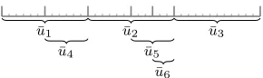
must be of dimension X−X0. Parts (a) and (b) of Figure 1 provide a partial illustration of how a pair of valuesρ and Ξ0 can be used to define a new, more granular partition.
Before proceeding we require one more definition. For each partition Ξk defined above,
where 0 ≤ k ≤ n, we introduce a collection of subsets of S denoted ¯Ξk = {X¯j : 1 ≤j ≤
X0+k}. Each element of ¯Ξk is defined as follows:
¯
Xj := (
{si:si ∈ Xj,0} if 1≤j≤X0
{si:si ∈ Xj,j−X0} ifX0< j ≤X
Each set ¯Xj is not a function of k. However, for j > X0 the value of ¯Xj will only be
available after j−X0 steps in the sequence described above. The effect of the definition is that, for 0≤ j ≤X0, we simply have ¯Xj =Xj,0 for all j, whilst for X0 < j ≤ X, ¯Xj will
contain all of the states which are contained in ¯Xj,j−X0, which is the first cell created during
the overall splitting process which had an index ofj, as it was before any additional splitting of that cell. (In other words, all the base cells can be referred to by ¯Xj for 1 ≤ j ≤ X0, and, for j > X0, each time a cell Xi,j−X0−1 is split, the newly created cell Xj,j−X0 is equal
to ¯Xj, while ¯Xi remains unchanged and still retains its value from the first time it was
created.) Note that ¯Ξk is not a partition, with the single exception of ¯Ξ0 which is equal
to Ξ0. The notation just outlined will be important when we set out the manner in which PASA estimates the frequency with which different cells are visited.
2.4. Details of the Algorithm
We now add the necessary final details to formally define the PASA algorithm. We assume we have a fixed ordered partition Ξ0 containing X0 cells. The manner in which Ξ0 is constructed does not need to be prescribed as part of the PASA algorithm, however we assume |Xj,0| ≥1 for all 1 ≤j ≤X0. In general, therefore, Ξ0 is a parameter of PASA.29 PASA stores a split vector ρ of dimension X−X0. This vector in combination with Ξ0 defines a partition Ξ, which will represent the state aggregation architecture used by the underlying SARSA algorithm. Recall that we usedXj to denote a cell in a state aggregation
architecture in Section 2.1. In the context of SARSA-P, Xj will be a function oft, and we
will use the natural convention thatXj =Xj,X−X0. We also adopt the notation ¯Ξ := ¯ΞX−X0.
The vector ρ, and correspondingly the partition Ξ, will be updated every ν ∈ N iter-ations, where ν (as noted above) is a fixed parameter. The interval defined by ν permits PASA to learn visit frequency estimates, which will be used when updating ρ. Subject to the constraint noted in the previous subsection,ρ can be initialised arbitrarily, however we assume that each ρk for 1≤k≤X−X0 is initialised so that no attempt will be made to
split a cell containing only one state (a singleton cell).
To assist in updating ρ, the algorithm will store a vector ¯u of real values of dimension X (initialised as a vector of zeroes). We update ¯u in each iteration as follows (i.e. using a simple stochastic approximation algorithm):
¯
u(jt+1)= ¯u(jt)+ςI{s(t)∈X¯j}−u¯
(t)
j
, (5)
whereς ∈(0,1] is a constant step size parameter. In this way, ¯uwill record the approximate frequency with which each of the sets in ¯Ξ have been visited by the agent.30 We also store an X dimensional boolean vector Σ. As will be made clearer below, Σ keeps track of whether a particular cell has only one state, as we don’t want the algorithm to try to split singleton cells.
29. The reason we do not simply takeX0= 1 is that takingX0>1 can help to ensure that the values stored
by PASA tend to remain more stable. In practice, it often makes sense to choose a suitable value for
X0, then simply take Ξ0 to be the ordered partition consisting ofX0 cells which are as close as possible
to equal size. See Section 4.
To updateρthe PASA algorithm, whenevertmodν = 0, performs a sequence ofX−X0 operations. A temporary copy of ¯u is made, which we call u. The vector u is intended to estimate the approximate frequency with which each of the cells in Ξ have been visited by the agent. The elements ofuwill be updated as part of the sequence of operations which we will presently describe. We set the entries of Σ toI{|Xk,0|=1} for 1≤k≤X0 at the start of
the sequence (the remaining entries can be set to zero). At each stagek∈ {1,2, . . . , X−X0} of the sequence we update ρ as follows:
ρk= (
j if (1−Σρk)uρk <max{ui :i≤X0+k−1,Σi= 0} −ϑ
ρk otherwise
(6)
where:
j= arg max
i
{ui :i≤X0+k−1,Σi= 0}
(if multiple indices satisfy the arg max function, we take the lowest index) and whereϑ >0 is a constant designed to ensure that a (typically small) threshold must be exceeded before ρ is adjusted. In this way, in each stepk in the sequence the non-singleton cellXj,k−1 with the highest valueuj (over the range 1≤j≤k−1, and subject to the threshold ϑ) will be
identified, via the update toρ, as the next cell to split. In each step of the sequence we also updateu and Σ:
uρk =uρk−uX0+k
Σj =I{|Xj,k|≤1} for 1≤j ≤X0+k−1.
The reason we update u as shown above is because each time the operation is applied we thereby obtain an estimate of the visit frequency ofXρk,k, which is the freshly updated value of uρk, and an estimate of the visit frequency of the cell XX0+k,k, which is uX0+k = ¯uX0+k
(sinceuX0+k = ¯uX0+kat stepk). We note that, for each of the cell visit frequency estimates
uρk and uX0+k to be accurate, it is critical that both the original estimates uρk anduX0+k
are accurate. Crucial to the operation of the algorithm is the fact that this dependence only flows in one direction. As estimates for larger cells tend to become more accurate, estimates for smaller cells which are a function of the estimates for larger cells also become more accurate. As a result we can depend upon accurate estimates for larger cells flowing through to accurate estimates for smaller cells. We might ask why we do not, for example, estimate the visit frequency of a newly created cell by simply dividing the visit frequency for the parent cell in two. This makes sense the first time a split is generated (and indeed doing this the first time a cell is split represents a sensible extension of the algorithm, see Section A.5), however, adopting the method we have described permits us to obtain estimates which will be exact in the limit as the algorithm is given time to converge.
Once ρhas been generated, we implicitly have a new partition Ξ. The PASA algorithm is outlined in Algorithm 1 and a diagram illustrating the main steps is at Figure 1. Note that the algorithm calls a procedure calledSplit, which is outlined in Algorithm 2.31 Algorithm
1 operates such that the cell splitting process (to generate Ξ) occurs concurrently with the update to ρ, such that, as each element ρk of ρ is updated, a corresponding temporary
partition Ξkis constructed. Also note that the algorithm makes reference to objects Ξ0 and
¯
Ξ0. To avoid storing each Ξk and ¯Ξk for 1≤k≤X−X0, we instead initialise Ξ0 and ¯Ξ0 as Ξ0 and then recursively update Ξ0 and ¯Ξ0 such that Ξ0 = Ξk and ¯Ξ0 = ¯Ξk at thekth stage
of the splitting process.
In Section 2.2 we noted that estimating the visit probability of individual cells by sub-tracting estimates from one another (as PASA is designed to do) allows us to avoid storing visit probabilities for S individual states. There is a trade-off involved when estimating visit frequencies in such a way. Suppose that t=nν for somen∈N and the partition Ξ(t) is updated and replaced by the partition Ξ(t+1). The visit frequency estimate for a cell in Ξ(t+1) is only likely to be accurate if the same cell was an element of Ξ(t), or if the cell is a union of cells which were elements of Ξ(t). Cells in Ξ(t+1) which do not fall into one of these categories will need time for an accurate estimate of visit frequency to be obtained (this will be shown more clearly in Section 3.2). The consequence is that it may take longer for the algorithm to converge (assuming fixed π) than would be the case if an estimate of the visit frequency of every state were available. The negative impact of this trade-off in practice does not appear to be significant (see Section 4), however the trade-off is essential to ensure we have an efficient algorithm from the perspective of space complexity.
3. Theoretical Analysis
Having proposed the PASA algorithm we will now investigate some of its theoretical prop-erties. With the exception of our discussion around complexity, these results will be con-strained to problems of policy evaluation, where π is held fixed and the objective is to minimise VF error. A summary of all of the theoretical results can be found in Table 1.
3.1. Complexity of PASA
PASA requires only a very modest increase in computational resources compared to fixed state aggregation. In relation to time complexity, ¯u can be updated in parallel with the SARSA algorithm’s update of θ (and the update of ¯u would not be expected to have any greater time complexity than the update to θ by SARSA, or indeed another standard RL algorithm such asQ-learning). Indeed, once a state has been mapped to a cell, the SARSA and PASA operations each have O(1) time complexity in relation toS.
X1,0 X2,0 X3,0
(a) We will have X0 = 3 “base” cells
in an ordered partition Ξ0. We will use
an arbitrarily chosen initial vectorρto split these cells and obtainX= 6 cells.
X1,3 X4,3 X2,3X5,3X6,3 X3,3
(b) Supposeρ is initialised (before the first iteration) asρ= (1,2,5). This de-fines a sequence of splits to arrive atX
cells depicted above. This partition rep-resents the initial value of Ξ, Ξ(1).
¯
u1 u¯2 u¯3
¯
u4 ¯u5
¯
u6
(c) Over the intervalt∈(1, . . . , ν), up-date the vector ¯u, an estimate of visit probabilities, then at iteration ν make a copy of ¯u,u.
u1=¯u1 u2=¯u2 u3=¯u3
∗
(d) At iteration ν we also generate a new value for ρ and Ξ. Start by split-ting the cell with the highest value of
ui (1≤i≤3). Assume this isu1. The
split, shown in red and with an asterisk, replaces a cell containing 12 states with two cells containing 6 states.
u2=¯u2 u3=¯u3
u1=¯u1−¯u4
u4=¯u4
∗
(e) Recalculateuand then split the cell with the next highest value of ui (for
1≤i≤4). Assume this isu3.
u2=¯u2
u1=¯u1−u¯4
u4=¯u4
u3=¯u3−u¯5
u5=¯u5
∗
(f) Repeat (for 1 ≤ i ≤ 5). In general this step will be repeatedX−X0 times.
u2=¯u2
u1=¯u1−¯u4
u4=¯u4
u3=¯u3−u¯5−u¯6
u5=¯u5
u6=¯u6
(g) This defines a new split vectorρand partition Ξ. In this caseρ= (1,3,3).
¯
u1 u¯2 u¯3
¯
u4 u¯6 u¯5
(h) Generate a new estimate ¯uover the intervalt∈(ν+1, . . . ,2ν), and continue the process indefinitely.
Algorithm 1The PASA algorithm, called at each iterationt. We assume ¯u,ρ, Ξ0, Ξ0and ¯Ξ0 are stored in memory. By definition ¯Ξ0 = Ξ0. The value of the partition Ξ0 at the conclusion of the function call will be used at t+ 1 to determine the state aggregation approximation architecture employed by SARSA. The valuesς,ϑ, andν are constant parameters. Initialise c(a counter) at zero. Initialise each element of the vector ¯uat zero. Denotes=s(t). Return is void.
1: function PASA(s)
2: for k∈ {1, . . . , X} do
3: u¯k ←u¯k+ς(I{s∈X¯k}−u¯k) . Update estimates of visit frequencies
4: end for 5: c←c+ 1
6: if c=ν then . Periodic updates toρ and Ξ 7: c←0
8: u←u¯ 9: Ξ0 ←Ξ0 10: Ξ¯0 ←Ξ0
11: fork∈ {1, . . . , X0}do
12: Σk←I{|Xk,0|=1} . Reset flags used to identify singular cells
13: end for
14: . Iterate through sequence of cell splits 15: fork∈ {1, . . . , X−X0}do
16: . Identify the cell with the highest visit probability estimate 17: umax←max{ui:i≤X0+k−1,Σi= 0}
18: imax←min{i:i≤X0+k−1, ui=umax,Σi = 0}
19: . If thresholdϑ is exceeded, update partition 20: if (1−Σρk)uρk < uimax −ϑthen
21: ρk ←imax . Reassign value forρ
22: end if
23: uρk ←uρk −uX0+k . Update value ofu
24: (Ξ0,Ξ¯0,Σ)←Split(k, ρk,Ξ0,Ξ¯0,Σ) .Call function to split cell
25: end for
26: end if 27: end function
Algorithm 2 Function to split selected cell in step k of sequence of cell splits. Called by PASA. The values Ξ00 and ¯Ξ00 are uninitialised and haveX0+kelements each. Use Xj0,Xj00,
¯
Xj0 and ¯Xj00 to denote the jth element of Ξ0, Ξ00, ¯Ξ0 and ¯Ξ00 respectively.
1: function Split(k,ρk,Ξ0,¯Ξ0,Σ)
2: . Set all but last element of Ξ00 and ¯Ξ00 3: for j∈ {1, . . . , X0+k−1} do
4: Xj00← Xj0 5: X¯j00←X¯j0 6: end for
7: L←min{i:si ∈ Xρk} .Determine cell end points
8: U ←max{i:si ∈ Xρk}
9: . Update Ξ00 10: Xρ00
k ← {si :L≤i≤L+b(U −L−1)/2c}
11: XX00
0+k← {si:L+b(U −L−1)/2c< i≤U}
12: . Set last element of ¯Ξ00 13: X¯X00
0+k← {sj :L+b(U−L−1)/2c< i≤U} .
¯
X00
ρk does not change
14: . Identify singular cells (only need to update values for newly split cells) 15: Σρk =I{|Xρk00|=1}
16: Σk=I{|X00 X0+k|=1}
17: return (Ξ00,Ξ¯00,Σ) .Return new partitions
18: end function
introduction of PASA as a pre-processing algorithm will not materially impact overall space requirements (in particular ifA is large).
3.2. Convergence Properties of PASA
We would now like to consider some of the convergence properties of PASA. We will assume, for our next result, thatπis held fixed for allt. There may be some potential to reformulate the result without relying on the assumption of fixed π, however our principle interest will be in this special case.
Our outline of PASA assumed a single fixed step size parameterς. For our proof below it will be easier to suppose that we have a distinct fixed step size parameter ςk for each
element ¯uk of ¯u (1 ≤ k ≤ X), each of which we can set to a different value (fixed as a
function oft). For the remainder of this section ς should be understood as referring to this vector of step size parameters. We use [1:k] to denote the set of indices from 1 tok, so that, for example, we can use x[1:k] to indicate a vector comprised of the first k elements of an arbitrary vector x. We will require some definitions.
Definition 1 We will say that some function oft, x=x(t),becomesε-fixed overτ afterT
providedT is such that, for allT0 > T, the value xwill remain the same for all t0 satisfying
T0 ≤t0 ≤T0+τ with probability at least1−ε. We will similarly say, given a set of values
valuex is equal to a single element ofRfor allt0 satisfyingT0 ≤t0 ≤T0+τ with probability
at least 1−ε.
Definition 1 provides the sense in which we will prove the convergence of PASA in Proposition 4. It is weaker than most conventional definitions of convergence, however it will give us conditions under which we can ensure thatρwill remain stable (i.e. unchanging) for arbitrarily long intervals with arbitrarily high probability. This stability will allow us to call on well established results relating to the convergence of SARSA with fixed state aggregation. Such a convergence definition also permits a fixed step size parameter ς. This means, amongst other things, that the algorithm will “re-converge” if P or (more importantly) π change.
Definition 2 We define µj,k := P
i:si∈Xj,kψi. We also define ρ˜ = ˜ρ(π) as the set of all
split vectors which satisfy ρ˜k = j ⇒ µj,k−1 ≥ µj0,k−1 for all 1 ≤ j0 ≤ X0 +k−1 and all
1≤k≤X−X0.
The valueµj,k =µj,k(π) is the stable state probability of the agent visiting states in the
cellXj,k (assuming some policyπ). This definition will be important as PASA progressively generates an estimate of this value, using the vectors u and ¯u. The set ˜ρ is the set of all split vectors which make the “correct” decision for each cell split (i.e. for some ρ∈ρ, the˜ cell in Ξk−1 with index ρk has the equal highest stable-state visit probability of all the cells
in Ξk−1 for 1≤k≤X−X0). The set ˜ρ[1:k] is defined such that ρ[1:k]∈ρ˜[1:k]if and only if there existsρ0∈ρ˜such thatρ[1:0 k]=ρ[1:k]. We require one final definition.
Definition 3 If, for each 1≤i≤X0+k, and for all ε >0, h >0 andτ ∈N, there exists
ς[1:(X0+k)], Hi (a closed interval on the real line of length h which satisfies µi,0 ∈ Hi for
i≤X0 and µi,i−X0 ∈Hi for X0 < i≤X) and Ti such that each
Ii :=I{u¯i∈Hi}
is ε-fixed over τ after Ti we will say that u¯ can be stabilised up to k. Similarly if for allε
and τ there exists ς[1:(X0+k−1)], ϑ >0 and T such that ρ[1:k] is ε-fixed at ρ˜[1:k] over τ after
T we will say that ρ can be uniquely stabilised up tok.
The implications of this definition are as follows. If ¯ucan be stabilised up tok, it means we can find values ς[1:(X0+k)] (likely to be small) such that we can ensure that the value
of each ¯ui for 1 ≤ i ≤ X0 +k will, with high probability, eventually come to rest within a small interval Hi of the real line. Similarly, if ρ can be uniquely stabilised up to k, it
implies that we can find valuesς[1:(X0+k−1)]and ϑ(the value for ϑis also likely to be small)
so thatρ[1:k] will eventually remain at a fixed value with the properties of ˜ρ (i.e. such that each split is “correct”) with high probability for a long period. The reason for introducing the index k into our definition is because our arguments below, wherein we establish that ρ will converge in the sense described in Definition 1, will depend on induction, and an interdependence between the elements of ¯u and ρ.
Proposition 4 For any particular instance of the pair (P, π), for every τ ∈ N and ε >
0, there exists ς, ϑ > 0 and T such that the vector ρ(t) generated by a PASA algorithm
Proof We will argue by induction. We will want to establish each of the following partial results, from which the result will follow: (1) ¯u can be stabilised up to 0; (2) For 1≤k≤
X−X0, if ¯u can be stabilised up tok−1, then ρ can be uniquely stabilised up to k; and, (3) For 1≤k≤X−X0, if ¯ucan be stabilised up tok−1 then ¯ucan be stabilised up tok. We begin with (1). We can argue this by relying on results regarding stochastic ap-proximation algorithms with fixed step sizes. We rely on the following (much more general) result: Theorem 2.2 in Chapter 8 of Kushner and Yin (2003). We will apply the result to each ¯ui (for 1 ≤i ≤X0). The result requires that a number of assumptions hold (see
Appendix A.1 where we state the assumptions and verify that they hold in this case) and states, in effect for our current purposes, the following.32 For all δ > 0, the fraction of iterations the value of ¯ui will stay within aδ-neighbourhood of the limit set of the ordinary
differential equation (ODE) of the update algorithm for ¯ui over the interval{0, . . . , T}goes
to one in probability as ςi → 0 and T → ∞. Recalling that, for all 1 ≤ i ≤ X0, ¯ui is
initialised at zero, in our case the ODE is µi,0(1−e−t) and the limit set is the point µi,0 (this statement can be easily generalised to any initialisation of ¯ui). The result therefore
means that for anyτ,handεwe can, for each ¯ui, chooseTi,ςi and findHi3µi,0 such that Ii will beε-fixed overτ after Ti, such that (1) holds.
We now look at (2). To see this holds, we elect arbitrary values τ0 and ε0 for which we need to find suitable values T0,ϑ and ς[1:(0 X
0+k−1)]. Suppose we set 0 <2ϑ≤min{|µj,k
0−
µj0,k0|: 0≤k0≤k−1,1≤j ≤X0+k0,1≤j0 ≤X0+k0, µj,k0 =6 µj0,k0} (ifµj,k0 is the same
for all j for all k0, any value ϑ > 0 can be chosen). Furthermore, using our assumption regarding ¯u, we selecth < ϑ/2k, noting that, if each ¯ui for 1≤i≤k−1 remains within an
interval of sizeϑ/2kfor the set of iterationsT0 ≤t≤T0+τ0, then eachui for 1≤i≤X0+k0
(for each generated value ofu in stepk0 of the sequence of updates ofu fork0 ≤k−1) will remain in an interval of lengthϑ/2 over the same set of iterations (since each ui will be a
set of additions of these values).
For any k0 ≤ k −1, define imax := arg maxi{µi,k0 : 1 ≤ i ≤ X0 +k0} (taking the
lowest index if this is satisfied by more than one index). If, for any 1 ≤ i0 ≤ X0 +k0, µi0,k0 6=µi
max,k0, then, provided each ¯ui for 1≤i≤X0+k
0 remains in an interval of length
h over the iterationsT0 ≤t≤T0+τ0:
u(it)
max−u
(t)
i0 ≥µimax,k0−h(k
0+ 1)− µ
i0,k0+h(k0+ 1)
≥2ϑ−2h(k0+ 1)> ϑ,
for the value of u at step k0 and for all t satisfying T0 ≤ t ≤T0+τ0 so that ρk0 ∈ ρ˜k0 for
T0 ≤t≤T0+τ0 for all 1≤k0 ≤k, where ˜ρk0+1 is the set of integers{m:ρk0+1=m, ρ∈ρ˜}.
Again for any k0 ≤k−1, if, for some i0, µimax,k0 =µi0,k0, let’s assume (without loss of
generality) that ρ(kT0+10) = imax. We will have, again provided each ¯ui for 1 ≤ i ≤ X0 +k0 remains in an interval of length h over the iterationsT0 ≤t≤T0+τ0:
u(it0)−u
(t)
imax ≤µi0,k0+h(k
0
+ 1)− µimax,k0−h(k
0
+ 1)
< µi0,k0+ϑ
2 −
µimax,k0 −
ϑ 2
=ϑ,
32. The result is in fact stated with reference to a time-shifted interpolated trajectory of ¯ui, where the
trajectory of ¯ui is uniformly interpolated between each discrete point in the trajectory and then scaled
for alltsatisfyingT0≤t≤T0+τ0which implies thatρk0+1will not change forT0 ≤t≤T0+τ0
for all 1 ≤ k0 ≤ k. As a result if we choose, from our assumed condition regarding ¯u, ε so that (1−ε)X0+k−1 ≥ 1−ε0, and we choose τ = τ0 +ν (to allow for the interval
delay before ρ is updated), then (2) is satisfied, since we can choose T0 = maxiTi and
ς[1:(0 X
0+k−1)]=ς[1:(X0+k−1)] whereς[1:(X0+k−1)] and eachTi are chosen to satisfy our choices
forεand τ.
Finally, we examine (3). Suppose we choose the valuesτ,handεand must find suitable valuesςi,Ti andHi (for 1≤i≤X0+k). By assumption, for each ¯ui for 1≤i≤X0+k−1, we can find suitable values in order to satisfy the condition. However we also know, from the arguments in (2), that by selecting suitable valuesε1,h1 andτ1 to which our assumption regarding ¯ui for 1≤i≤X0+k−1 applies, we can ensure, for any values of ε2 andτ2, that ρ[1:k] will beε2-fixed overτ2 after T for some T. Note that if, for somei,Ii is ε-fixed over
τ afterT for some Hi of lengthhthenIi will also beε0-fixed over τ0 afterT for some Hi0 of
lengthh0 for anyε0 > ε,τ0< τ andh0 > h. This last observation means that we can choose ε0,h0 and τ0 so thatε0 < ε1,ε0< ε,h0 < h1,h0 < h,τ0 > τ1 and τ0 > τ, so that, for any ε2,τ2,ε,h andτ, we can find suitable valuesςi,Ti andHi (for 1≤i≤X0+k−1) so that all conditions are satisfied.
Again relying on the result from Kushner and Yin (2003), for any ε3, h and τ there existsςX0+k,HX0+kof lengthh andT
00 which will ensure that ¯u
X0+k will remain inHX0+k
with probability at least 1−ε3 for alltsuch thatT00≤t≤T00+τ, provided the value ofρk0
for 1≤k0 ≤kis held fixed for allt≤T00+τ, for any starting value of ¯ukbounded by the
in-terval [−1,1] (the limit set of the ODE is the same for all such starting values, and since the interval is compact we can choose the minimum valueςX0+krequired to satisfy the condition
for all starting values). Now, we can choose ε2 and ε3 such that (1−ε)>(1−ε2)(1−ε3) and chooseτ2 such that τ2 ≥T00+τ. In this way, given the value of ςX0+k shown to exist
above and TX0+k ≥maxiTi+T
00 we will have the required values to ensure the necessary
property also holds for ¯uX0+k.
Since ρ completely determines Ξ the result implies the convergence of Ξ to a partition Ξlim. This fact means that SARSA-P will converge if π is held fixed (this is discussed in more detail below). Moreover a straightforward extension of the arguments in Gordon (2001) further implies that SARSA-P will not diverge even whenπ is updated. The result also implies that Ξlim will have the property that more frequently visited states will, in general, occupy smaller cells.
Note again that we have taken care to allow the vector ς to remain fixed as a function of t. This will, in principle, allow PASA to adapt to changes in π (assuming we allowπ to change). We will use fixed step sizes in our experiments below. Whilst in our experiments in Section 4 we use only a single step size parameter (as opposed to a vector), the details of the proof above point to why there may be merit in using a vector of step size parameters as part of a more sophisticated implementation of the ideas underlying PASA (i.e. allowingςk
to take on larger values for larger values of the indexk, fork > X0, may allow the algorithm to converge more rapidly).