Robust Estimation of Derivatives Using Locally Weighted
Least Absolute Deviation Regression
WenWu Wang [email protected]
School of Statistics Qufu Normal University
Jingxuan West Road, Qufu, Shandong, China
Ping Yu [email protected]
Faculty of Business and Economics University of Hong Kong
Pokfulam Road, Hong Kong
Lu Lin [email protected]
Zhongtai Securities Institute for Financial Studies Shandong University
Jinan, Shandong, China
Tiejun Tong [email protected]
Department of Mathematics Hong Kong Baptist University Kowloon Tong, Hong Kong
Editor:Zhihua Zhang
Abstract
In nonparametric regression, the derivative estimation has attracted much attention in re-cent years due to its wide applications. In this paper, we propose a new method for the derivative estimation using the locally weighted least absolute deviation regression. Dif-ferent from the local polynomial regression, the proposed method does not require a finite variance for the error term and so is robust to the presence of heavy-tailed errors. Mean-while, it does not require a zero median or a positive density at zero for the error term in comparison with the local median regression. We further show that the proposed estimator with random difference is asymptotically equivalent to the (infinitely) composite quantile regression estimator. In other words, running one regression is equivalent to combining infinitely many quantile regressions. In addition, the proposed method is also extended to estimate the derivatives at the boundaries and to estimate higher-order derivatives. For the equidistant design, we derive theoretical results for the proposed estimators, including the asymptotic bias and variance, consistency, and asymptotic normality. Finally, we conduct simulation studies to demonstrate that the proposed method has better performance than the existing methods in the presence of outliers and heavy-tailed errors, and analyze the Chinese house price data for the past ten years to illustrate the usefulness of the proposed method.
Keywords: composite quantile regression, differenced method, LowLAD, LowLSR, out-lier and heavy-tailed error, robust nonparametric derivative estimation
c
1. Introduction
The derivative estimation is an important problem in nonparametric regression and it has applications in a wide range of fields. For instance, when analyzing human growth data (M¨uller, 1988; Ramsay and Silverman, 2002) or maneuvering target tracking data (Li and Jilkov, 2003, 2010), the first- and second-order derivatives of the height as a function of time are two important parameters, with the first-order derivative representing the speed and the second-order derivative representing the acceleration. The derivative estimates are also needed in change-point problems, e.g., for exploring the structures of curves (Chaudhuri and Marron, 1999; Gijbels and Goderniaux, 2005), for detecting the extremum of derivatives (Newell et al., 2005), for characterizing submicroscopic nanoparticle from scattering data (Charnigo et al., 2007, 2011a), for comparing regression curves (Park and Kang, 2008), for detecting abrupt climate changes (Matyasovszky, 2011), and for inferring the cell growth rates (Swain et al., 2016).
In the existing literature, one usually obtains the derivative estimates as a by-product by taking the derivative of a nonparametric fit of the regression function. There are three main approaches for the derivative estimation: smoothing spline, local polynomial regression, and differenced estimation. For smoothing spline, the derivatives are estimated by taking derivatives of the spline estimation of the regression function (Stone, 1985; Zhou and Wolfe, 2000). For local polynomial regression, a polynomial using the Taylor expansion is fitted locally by the kernel method (Ruppert and Wand, 1994; Fan and Gijbels, 1996; Delecroix and Rosa, 1996). These two methods both require an estimate of the regression function. As pointed out in Wang and Lin (2015), when the regression function estimator achieves the optimal rate of convergence, the corresponding derivative estimators may fail to achieve the rate. In other words, minimizing the mean square error of the regression function estimator does not necessarily guarantee the derivatives be optimally estimated (Wahba and Wang, 1990; Charnigo et al., 2011b).
For the differenced estimation, M¨uller et al. (1987) and H¨ardle (1990) proposed a cross-validation method to estimate the first-order derivative without estimating the regression function. Unfortunately, their method may not perform well in practice as the variance of their estimator is proportional to n2 when the design points are equally spaced. Observ-ing this shortcomObserv-ing, Charnigo et al. (2011b) and De Brabanter et al. (2013) proposed a variance-reducing estimator for the derivative function called the empirical derivative that is essentially a linear combination of the symmetric difference quotients. They further de-rived the order of the asymptotic bias and variance, and established the consistency of the empirical derivative. Wang and Lin (2015) represented the empirical derivative as a local constant estimator in locally weighted least squares regression (LowLSR), and proposed a new estimator for the derivative function to reduce the estimation bias in both valleys and peaks of the true derivative function. More recently, Dai et al. (2016) generalized equidis-tant design to non-equidisequidis-tant design, and Liu and De Brabanter (2018) further generalized the existing work to random design.
ex-ample, kernel M-smoother (H¨ardle and Gasser, 1984), local least absolute deviation (LAD) (Fan and Hall, 1994; Wang and Scott, 1994), and locally weighted least squares (Cleveland, 1979; Ruppert and Wand, 1994) among others. In contrast, little attention has been paid to improving the derivative estimation except for the parallel developments of the above remedies (H¨ardle and Gasser, 1985; Welsh, 1996; Boente and Rodriguez, 2006), so call for a better solution.
In this paper, we propose a locally weighted least absolute deviation (LowLAD) method by combining the differenced method and theL1regression systematically. Over a neighbor-hood centered at a fixed point, we first obtain a sequence of linear regression representation in which the derivative is the intercept term. We then estimate the derivative by minimizing the sum of weighted absolute errors. By repeating this local fitting over a grid of points, we can obtain the derivative estimates on a discrete set of points. Finally, the entire deriva-tive function is obtained by applying the local polynomial regression or the cubic spline interpolation.
The rest of the paper is organized as follows. Section 2 presents the motivation, the first-order derivative estimator and its theoretical properties, including the asymptotic bias and variance, consistency, and asymptotic normality. Section 3 studies the relation between the LowLAD estimator and the existing estimators. In particular, we show that the LowLAD estimator with random difference is asymptotically equivalent to the (infinitely) composite quantile regression estimator. Section 4 derives the first-order derivative estimation at the boundaries of the domain, and Section 5 generalizes the proposed method to estimate the higher-order derivatives. In Section 6 we conduct extensive simulation studies to assess the finite-sample performance of the proposed estimators and compare them with the existing competitors; we also apply our method to a real data set to illustrate its usefulness in practice. Finally, we conclude the paper with some discussions in Section 7, and provide the proofs of the theoretical results in six Appendices.
A word on notation: = means that the higher-order terms are omitted, and. ≈ means an approximate result with up to two decimal digits.
2. First-Order Derivative Estimation
Combining the differenced method and theL1 regression, we propose the LowLAD regres-sion to estimate the first-order derivative. The new method inherits the advantage of the differenced method and also the robustness of the L1 method.
2.1. Motivation
Consider the nonparametric regression model
Yi =m(xi) +i, 1≤i≤n, (1)
We first define first-order symmetric (abouti) difference quotient (Charnigo et al., 2011b; De Brabanter et al., 2013) as
Yij(1)= Yi+j−Yi−j
xi+j−xi−j
, 1≤j ≤k, (2)
wherek is a positive integer, and then decompose Yij(1) into two parts as
Yij(1)= m(xi+j)−m(xi−j) 2j/n +
i+j−i−j
2j/n , 1≤j ≤k. (3)
On the right hand side of (3), the first term contains the bias information of the true deriva-tive, and the second term contains the variance information. By Wang and Lin (2015), the first-order derivative estimation based on the third-order Taylor expansion usually outper-forms the estimation based on the first-order Taylor expansion due to bias correction. For the same reason, we assume that m(·) is three times continuously differentiable on [0,1]. By the Taylor expansion, we obtain
m(xi+j)−m(xi−j) 2j/n =m
(1)(x i) +
m(3)(xi) 6
j2 n2 +o
j2 n2
, (4)
where the estimation bias is contained in the remainder term of the Taylor expansion. By (3) and (4), we have
Yij(1) =m(1)(xi) +
m(3)(xi) 6
j2 n2 +
i+j−i−j 2j/n +o
j2 n2
. (5)
In Proposition 11 (see Appendix A), we show that the median ofi+j−i−j is always zero, no matter whether the median of i is zero or not. As a result, for any fixed k=o(n), we have
Median[Yij(1)] =m(1)(xi) +
m(3)(xi) 6 d
2
j+o d2j
, 1≤j ≤k, (6)
where dj = j/n. We treat (6) as a linear regression with d2j and Y (1)
ij as the independent and dependent variables, respectively. In the presence of heavy-tailed errors, we propose to estimate m(1)(xi) as the intercept of the linear regression using the LowLAD method. 2.2. Estimation Methodology
In order to derive the estimation bias, we further assume thatm(·) is five times continuously differentiable, that is, the regression function is two degrees smoother than our postulated model due to the equidistant design. Following the paradigm of Draper and Smith (1981) and Wang and Scott (1994), we discard the higher-order terms of m(·) and assume locally that the approximate model is
Yij(1) =βi1+βi3dj2+βi5d4j +ζij,
Median[ζij] = 0. Under the assumption of the approximate model, βi1 can be estimated as
min b
k X
j=1
wj Y
(1)
ij −(bi1+bi3d2j +bi5d4j) = min
b k X
j=1 Y˜
(1)
ij −(bi1dj +bi3d3j +bi5d5j) ,
wherewj =dj are the weights, b= (bi1, bi3, bi5)T, and ˜Yij(1) = (Yi+j−Yi−j)/2. Accordingly, the approximate model can be rewritten as
˜
Yij(1)=βi1dj+βi3d3j +βi5d5j+ ˜ζij,
where ˜ζij = (i+j −i−j)/2 are iid random errors with Median[ ˜ζij] = 0 and a continuous, symmetric densityg(·) which is positive in a neighborhood of zero (see Appendix A).
Rather than the best L1 quintic fitting, we search for the bestL1 cubic fitting to ˜Yij(1). Specifically, we estimate the model by LowLAD:
( ˆβi1,βˆi3) = arg min b
k X
j=1 Y˜
(1)
ij −bi1dj−bi3d3j
withb= (bi1, bi3)T, and define the LowLAD estimator ofm(1)(xi) as ˆ
m(1)LowLAD(xi) = ˆβi1. (7)
The following theorem states the asymptotic behavior of ˆβi1.
Theorem 1 Assume that i are iid random errors with a continuous bounded densityf(·). Then as k→ ∞ and k/n→0, βˆi1 in (7) is asymptotically normally distributed with
Bias[ ˆβi1] =−
m(5)(xi) 504
k4 n4 +o
k4 n4
, Var[ ˆβi1] = 75 16g(0)2
n2 k3 +o
n2 k3
,
where g(0) = 2R∞
−∞f2(x)dx. The optimal k that minimizes the asymptotic mean square error (AMSE) is
kopt≈3.26
1
g(0)2m(5)(x i)2
1/11
n10/11,
and, consequently, the minimum AMSE is
AMSE[ ˆβi1]≈0.19
m(5)(xi)6
g(0)16
!1/11
n−8/11.
In the local median regression (see Section 3.1 below for its definition), the density f(·) is usually assumed to have a zero median and a positive f(0) value. While in Theorem 1, we only require a continuity condition on the density f(·). In addition, the variance of the LowLAD estimator depends on g(0) = 2R∞
2.3. LowLAD with Random Difference
To further improve the estimation efficiency, we propose the LowLAD with random dif-ference referred to as RLowLAD. First, define the first-order random difdif-ference sequence as
Yijl =Yi+j−Yi+l, −k≤j, l≤k,
where we implicitly exclude j and l being 0 to be comparable to the LowLAD estimator. Second, define the RLowLAD estimator as
ˆ
m(1)RLowLAD(xi) = ˆβRLowLADi1 , (8) where
( ˆβi1RLowLAD,βˆi2RLowLAD,βˆi3RLowLAD,βˆi4RLowLAD) = arg min
b k X
j=−k k X
l=−k,l<j
Yijl−bi1(dj−dl)−bi2(d2j −d2l)−bi3(d3j −d3l)−bi4(d4j −d4l)
with the true valueβi = (βi1, βi2, βi3, βi4)T = (m(1)(xi), m(2)(xi)/2, m(3)(xi)/6, m(4)(xi)/24)T and b= (bi1, bi2, bi3, bi4)T.
Theorem 2 Under the assumptions of Theorem 1, the bias and variance of the RLowLAD estimator in (8) are, respectively,
Bias[ ˆβi1RLowLAD] =−m
(5)(x i) 504
k4 n4 +o
k4 n4
, Var[ ˆβi1RLowLAD] = 75 24g(0)2
n2 k3 +o
n2 k3
.
By replacing the symmetric difference with the random difference, we improve the esti-mation accuracy with the variance from 16g(0)75 2
n2
k3 to
75 24g(0)2
n2
k3. While the cost is to increase
the computation complexity from O(n) toO(n2).
3. Comparison with Existing First-Order Derivative Estimators
We first review some existing methods for the first-order derivative estimation which are based on either the least squares regression or the quantile regression. Both methods can be used to estimate the first-order derivative ofm(·) due to the special structure of model (1). Note that E [Yi|xi] =m(xi) + E [i], and Qτ(Yi|xi) =m(xi) + Qτ(i) becausei is inde-pendent ofxi, where Qτ(i) is theτth unconditional quantile of i. Although E [Yi|xi] may not equal to Qτ(Yi|xi), their derivatives must be the same as the corresponding derivatives of m(xi). To make the existing estimators comparable to our LowLAD and RLowLAD estimators, we use the uniform kernel and the same order Taylor expansion throughout this section.
3.1. LS, LowLSR and LAD Estimators
In Fan and Gijbels (1996), the first-order derivative is estimated by the least squares method:
( ˆαLSi0,αˆLSi1 ,αˆLSi2,αˆLSi3 ,αˆi4LS) = arg min α
k X
j=−k
Yi+j−αi0−αi1dj−αi2d2j−αi3d3j −αi4d4j 2
where α = (αi0, αi1, αi2, αi3, αi4)T. For ease of comparison, we exclude the point j = 0 so that the same Yi’s are used as in the LowLAD estimation. Define the least squares (LS) estimator as
ˆ
m(1)LS(xi) = ˆαLSi1. (9) Corollary 3 Under the assumptions of Theorem 1, the bias and variance of the LS esti-mator in (9)are, respectively,
Bias[ ˆαLSi1 ] =−m
(5)(x i) 504
k4 n4 +o
k4 n4
, Var[ ˆαLSi1 ] = 75σ 2 8
n2 k3 +o
n2 k3
.
To obtain the optimal convergence rate of the derivative estimation, Wang and Lin (2015) proposed the LowLSR estimator:
ˆ
m(1)LowLSR(xi) = ˆαLowLSRi1 , (10) where
( ˆαLowLSRi1 ,αˆLowLSRi3 ) = arg min αi1,αi3
k X
j=1
˜
Yij(1)−αi1dj−αi3d3j 2
.
Corollary 4 Under the assumptions of Theorem 1, the bias and variance of the LowLSR estimator in (10) are, respectively,
Bias[ ˆαLowLSRi1 ] =−m
(5)(x i) 504
k4 n4 +o
k4 n4
, Var[ ˆαLowLSRi1 ] = 75σ 2 8
n2 k3 +o
n2 k3
.
Wang and Scott (1994) proposed the local polynomial least absolute deviation (LAD) estimator:
ˆ
m(1)LAD(xi) = ˆβLADi1 , (11) where
( ˆβi0LAD,βˆLADi1 ,βˆi2LAD,βˆi3LAD,βˆi4LAD) = arg min b
k X
j=−k
Yi+j−bi0−bi1d1j−bi2d2j−bi3d3j−bi4d4j
withb= (bi0, bi1, bi2, bi3, bi4)T.
Corollary 5 Under the assumptions of Theorem 1, the bias and variance of the LAD es-timator in (11) are, respectively,
Bias[ ˆβi1LAD] =−m
(5)(x i) 504
k4 n4 +o
k4 n4
, Var[ ˆβi1LAD] = 75 32f(0)2
n2 k3 +o
n2 k3
.
3.2. Quantile Regression Estimators
Quantile regression (Koenker and Bassett, 1978; Koenker, 2005) exploits the distribution information of the error term to improve the estimation efficiency. Following the composite quantile regression (CQR) in Zou and Yuan (2008), Kai et al. (2010) proposed the local polynomial CQR estimator. In general, the local polynomial CQR estimator of m(1)(xi) is defined as
ˆ
m(1)CQR(xi) = ˆγi1CQR, (12) where
(
n
ˆ
γi0hCQR
oq h=1,γˆ
CQR i1 ,γˆ
CQR i2 ,ˆγ
CQR i3 ,ˆγ
CQR i4 )
= arg min γ q X h=1 k X j=−k
ρτh(Yi+j−γi0h−γi1d
1
j −γi2d2j −γi3d3j −γi4d4j)
,
with γ = {γi0h}qh=1, γi1, γi2, γi3, γi4 T
, ρτ(x) =τ x−xI(x <0) is the check function, and
τh =h/(q+ 1).
Corollary 6 Under the assumptions of Theorem 1, the bias and variance of the CQR estimator in (12) are, respectively,
Bias[ˆγi1CQR] =−m
(5)(x i) 504
k4
n4 +o
k4
n4
, Var[ˆγi1CQR] = 75R1(q) 8
n2
k3 +o
n2
k3
,
where R1(q) = Pql=1Pql0=1τll0/{Pq
l=1f(cl)}2, cl =F −1(τ
l), and τll0 = min{τl, τl0} −τlτl0.
As q→ ∞,
R1(q)→
1
12(E[f()])2 = 1
3g(0)2, Var[ˆγ CQR i1 ] =
75 24g(0)2
n2
k3 +o
n2
k3
.
Zhao and Xiao (2014) proposed the weighted quantile average (WQA) estimator for the regression function in nonparametric regression, an idea originated from Koenker (1984). We now extend the WQA method to estimatem(1)(xi) using the local polynomial quantile regression. Specifically, we define
ˆ
m(1)WQA(xi) = q X
h=1
whˆγi1hWQA, (13)
wherePq
h=1wh = 1, and
(ˆγi0hWQA,γˆi1hWQA,ˆγi2hWQA,γˆi3hWQA,ˆγi4hWQA) = arg min
γh k X j=−k
ρτh(Yi+j−γi0h−γi1hd
1
j −γi2hd2j −γi3hd3j−γi4hd4j)
Corollary 7 Under the assumptions of Theorem 1, the bias and variance of the WQA estimator in (13) are, respectively,
Bias[ ˆm(1)WQA(xi)] =−
m(5)(xi) 504
k4 n4++o
k4 n4
, Var[ ˆm(1)WQA(xi)] =
75R2(q|w) 8
n2 k3+o
n2 k3
,
where R2(q|w) = wTHw with w = (w1,· · ·, wq)T, and H =
n τ
ll0
f(cl)f(cl0)
o
1≤l,l0≤q. The
optimal weights are given by w∗ = H−1eq
eT
qH−1eq, where eq = (1, . . . ,1)
T
q×1, and R2(q|w∗) = (eTqH−1eq)−1. As q → ∞, under the regularity assumptions in Theorem 6.2 of Zhao and Xiao (2014), the variance of the optimal CQR is
Var[ ˆm(1)WQA(xi)] =
75I(f)−1 8
n2 k3 +o
n2 k3
,
where I(f) is the Fisher information of f.
LS LowLSR LAD CQR WQA LowLAD RLowLAD
s2 σ2 σ2 4f(0)1 2 R1(q) R2(q) 2g(0)1 2 3g(0)1 2
Asymptotics2 σ2 σ2 4f(0)1 2 3g(0)1 2 I(f)
−1 1
2g(0)2 3g(0)1 2
Table 1: s2 in the variances 75n2
8k3 s2 of the existing first-order derivative estimators.
For the LS, LowLSR, LAD, CQR, WQA, LowLAD and RLowLAD estimators with the same k, their asymptotic biases are all the same. In contrast, their asymptotic variances are 75n8k32s2 with s2 being σ2, σ2,4f(0)1 2, R1(q), R2(q), 2g(0)1 2 and 3g(0)1 2, as listed in Table
1. From the kernel interpretation of the differenced estimator by Wang and Yu (2017), we expect an equivalence between the LS and LowLSR estimators. As q → ∞, we have
R1(q) → 1/{3g(0)2} and R2(q) → I(f)−1, and hence the WQA estimator is the most efficient estimator asqbecomes large. Nevertheless, it requires the error density function to be known in advance to carry out the most efficient WQA estimator. Otherwise, a two-step procedure is needed, where the first step estimates the error density. For a fixed q, the three quantile-based estimators (i.e., LAD, CQR, WQA) depend only on the density values of f(·) at finite quantile points, whose behaviors are uncertain and may not be reliable. In contrast, our new estimators rely ong(0) = 2E[f(x)], which includes all information on the densityf(·) and hence is more robust.
3.3. Relationship Among the CQR, WQA and RLowLAD Estimators
the distribution of the error term ofYijlis R
f F−1(τ)
dτ, and then run a single regression horizontally (at τ = 0.5). It is interesting (and may be also surprising) to see that these two different ways of using information have the same efficiency. The RLowLAD estimation is more powerful in practice by noticing that a single differencing in Yijl is equivalent to combining all (infinitely many) quantiles.
It should be emphasized that the ways of combining the infinitely many quantiles in
CQR and WQA are different. Suppose we use the equal weights wE =
1
q,· · ·,
1 q
T
in WQA. Such a weighting scheme is parallel to CQR where an equal weight is imposed on each check function. Then from Theorem 2 of Kai et al. (2010),R2(q|wE)→1 as q → ∞; while R1(q) → 3g(0)1 2. From Table 2 of Kai et al. (2010), 3g(0)1 2 < 1 for most distributions
(except N(0,1)). Why can this difference happen? Note that
n ˆ
γWQAih
oq
h=1 = arg minγ1,···,γq
q X
h=1 k X
j=−k
ρτh(Yi+j−γi0h−γi1hd
1
j−γi2hd2j −γi3hd3j −γi4hd4j)
whereˆγihWQA = (ˆγi0hWQA,ˆγi1hWQA,γˆi2hWQA,ˆγi3hWQA,γˆi4hWQA)T, so the CQR estimator is a constrained WQA estimator with the constraints being that the slopes at different quantiles must be the same. On the other hand, the WQA estimator can be interpreted as a minimum distance estimator,
arg min γ
ˆ
γi1WQA−γeq T
W
ˆ
γi1WQA−γeq
= e T qWˆγ
WQA i1
eT qWeq
=wTˆγi1WQA,
where ˆγWQAi1 =γˆi11WQA,· · ·,ˆγi1qWQAT, W is a symmetric weight matrix, and w= Weq
eT qWeq.
When W = Iq, the q ×q identity matrix, we get the equally-weighted WQA estimator; when W=H−1, we get the optimally weighted WQA estimator; and when
W=aIq+ (1−a)H−1 6=Iq,
we get an estimator that is asymptotically equivalent to the CQR estimator, where
a= −(q−B) (1−BC) +
p
(q2−AB) (1−BC)
A−(2q−B) (1−BC)−q2C 6= 1 with A = eT
qHeq = q2R2(q|wE), B = R2(q|w∗)−1 and C = R1(q). For example, if
ε ∼ N(0,1), then when q = 5, a = −0.367; when q = 9, a = −0.165; when q = 19,
a= −0.067; and when q = 99, a= −0.011. This is why imposing constraints directly on the objective function (i.e., the CQR estimator) or on the resulting estimators (i.e., the WQA estimator) would generate different estimators. The RLowLAD estimator and the CQR estimator have the same asymptotic variance because both of them impose constraints directly on the objective function.
3.4. Asymptotic Relative Efficiency
Since all estimators have the same bias, the comparison of their variances becomes important. We define the variance ratios of the LowLSR and LAD estimators relative to the RLowLAD estimator as
RLowLSR =
Var( ˆmLowLSR(1))
Var( ˆm(1)RLowLAD)
= 3σ2g(0)2,
RLAD=
Var( ˆm(1)LAD) Var( ˆm(1)RLowLAD)
= 3g(0) 2 4f(0)2.
In addition, the overall performance of an estimator is usually measured by its AMSE, so we define the AREs based on AMSE as
ARELowLSR =
AMSE( ˆm(1)LowLSR) AMSE( ˆm(1)RLowLAD)
,
ARELAD =
AMSE( ˆm(1)LAD) AMSE( ˆm(1)RLowLAD)
.
The LowLSR estimator has the AMSE
AMSE( ˆm(1)LowLSR) =
(
m(5)(xi) 504
k4 n4
)2
+75σ 2 8
n2 k3, and the optimalkminimizing the AMSE is
kLowLSRopt =
893025σ2
(m(5)(x i))2
1/11
n10/11
Similarly, we have
kRLowLADopt =
893025 3g(0)2(m(5)(x
i))2 1/11
n10/11=R−1/11LowLSRkoptLowLSR.
Asn→ ∞, we can show
ARELowLSR = RLowLSR8/11, ARELAD= RLAD8/11.
Since the variance ratio and ARE have a close relationship, we only report the vari-ance ratios. We consider eight distributions for the random errors: the normal distribution
f(0) g(0) σ2 RLowLSR RLAD
N(0,1) 0.40 0.56 1 0.95 1.5 0.9N(0,1) + 0.1N(0,32) 0.37 0.50 1.8 1.37 1.38 0.9N(0,1) + 0.1N(0,102) 0.36 0.47 10.9 7.28 1.27
t(3) 0.37 0.46 3 1.90 1.17 Laplace 0.50 0.50 2 1.50 0.75 Logistic 0.25 0.33 3.29 1.10 1.33
Cauchy 0.32 0.32 ∞ ∞ 0.75
0.9Gamma(0,1) + 0.1Gamma(1,1) 0.50 0.45 1.1 1.63 0.68 0.9Gamma(0,1) + 0.1Gamma(3,1) 0.46 0.42 1.3 2.44 0.68 0.5N(−1,1) + 0.5N(1,1) 0.15 0.39 2 0.89 5.18 0.5N(−3,1) + 0.5N(3,1) 4.92×10⁻⁵ 0.28 10 2.39 2.46×10⁷
Table 2: Variance ratios for different error distributions.
Table 2 lists the variance ratios for these eight error distributions which are derived in Appendix E. From Table 2, a few interesting results can be drawn. First of all, the variance of the RLowLAD estimator is usually smaller and more robust than that of the LowLSR and LAD estimators in most cases. Secondly, the LAD estimator is not robust since it relies on the density value at one point 0, so when facing the bimodal errors the variance is huge. Thirdly, the minimum value of RLowLSR in Table 2 is 0.89. Actually, there is an exact lower bound for RLowLSRas stated in Theorem 4 of Kai et al. (2010). For completeness, we repeat their Theorem 4 in the following Lemma 8.
Lemma 8 Let F denote the class of error distributions with mean 0and variance 1. Then inf
f∈FRLowLSR(f)≈0.86.
The lower bound is reached if and only if the error follows the rescaledbeta(2,2)distribution. Thus,
inf
f∈FARELowLSR(f) = R 8/11
LowLSR≈0.90.
In other words, the potential efficiency loss of the RLowLAD estimator relative to the LowLSR estimator is at most 10%.
In Appendix E, we further illustrate the trade-off between the sharp-peak and heavy-tailed errors using three error distributions.
4. Derivative Estimation at Boundaries
At the left boundary with 2≤ i≤k, the bias and variance of the LowLAD estimator are
−m(5)(x
Assume that m(·) is twice continuously differentiable on [0,1] and Median[i] = 0. For 1≤i≤k, we define the asymmetric lag-j first-order difference quotients as
Yij<1>= Yi+j−Yi
xi+j−xi
, −(i−1)≤j ≤k, j 6= 0.
By decomposing Yij<1> into two parts, we have
Yij<1>= m(xi+j)−m(xi)
j/n +
i+j −i
j/n
=m(1)(xi) + (−i)d−1j +
i+j
j/n +
m(2)(xi) 2!
j n +o
j n
,
where i is fixed as j changes. Thus, Median(Yij<1>
i) = m(1)(xi) + (−i)d−1j +m
(2)(x
i)
2! j n. Ignoring the last term, we can rewrite the above model as
Yij<1>=βi1+βi0d−1j +δij+o(1), −(i−1)≤j≤k, j6= 0,
where (βi0, βi1)T = (−i, m(1)(xi))T, δij = j/ni+j. By the LowLAD method, the regression coefficients can be estimated as
ˆ
βi0,βˆi1
= arg min b
k X
j=−(i−1)
Yij<1>−bi1−bi0d−1j wj
= arg min b
k X
j=−(i−1)
Y˜ij<1>−bi0−bi1dj ,
(14)
where wj = dj, b = (bi0, bi1)T, and ˜Yij<1> = Yi+j −Yi. The As-LowLAD estimator of
m(1)(xi) is ˆβi1.
Similarly to Theorem 1, we can prove the asymptotic normality for ˆβi1. The following theorem states its asymptotic bias and variance.
Theorem 9 Assume thati are iid random errors with median0and a continuous, positive densityf(·) in a neighborhood of zero. Furthermore, assume thatm(·) is twice continuously differentiable on [0,1]. Then for each 1≤i≤k, the leading terms of the bias and variance of βˆi1 in (14) are, respectively,
Bias[ ˆβi1] =
m(2)(xi) 2
k4+ 2k3i−2ki3−i4 n(k3+ 3k2i+ 3ki2+i3), Var[ ˆβi1] =
3
f(0)2
n2
k3+ 3k2i+ 3ki2+i3.
For the estimation at the boundaries, Wang and Lin (2015) proposed a one-side LowLSR (OS-LowLSR) estimator of the first-order derivative, with the bias and variance being
and 3n2/(f(0)2k3), respectively. Note that the two biases are the same, while the variances are different with the former related to σ2 and the latter related to f(0). Note also that different from the LowLAD estimator at the interior point, the variance of the OS-LowLAD estimator involvesf(0) rather than g(0).
Theorem 9 shows that our estimator has a smaller bias than the LowLSR and OS-LowLAD estimators. In the special case i = k, the bias disappears (in fact it reduces to the higher-order term O(k2/n2)). With normal errors, when 1 < i < b0.163kc, the order of variances of the three estimators is Var( ˆm(1)OS−LAD(xi)) > Var( ˆm(1)AS−LAD(xi)) > Var( ˆm(1)OS−LSR(xi)), where for a real number x, bxc means the largest integer less than x; whenb0.163kc< i < k, the order of variances of the three estimators is Var( ˆm(1)OS−LSR(xi))> Var( ˆm(1)OS−LAD(xi)) > Var( ˆm(1)AS−LAD(xi)). As i approaches k, the variance of the As-LowLAD estimator is reduced to one-eighth of the variance of the OS-As-LowLAD estimator, and is much smaller than the variance of the OS-LowLSR estimator.
Up to now, we have the first-order derivative estimators {mˆ(1)(xi)}ni=1 on the discrete points{xi}ni=1. To estimate the first-order derivative function, we suggest two strategies for different noise levels of the derivative data: the cubic spline interpolation in Knott (2000) for ‘good’ derivative estimators, and the local polynomial regression in Brown and Levine (2007) and De Brabanter et al. (2013) for ‘bad’ derivative estimators. Here, the terms ‘good’ and ‘bad’ indicate small and large estimation variances of the derivative estimators, respectively.
5. Second- and Higher-Order Derivative Estimation
In this section, we generalize our robust method for the first-order derivative estimation to the second- and higher-order derivatives estimation.
5.1. Second-Order Derivative Estimation Define the second-order difference quotients as
Yij(2) = Yi−j−2Yi+Yi+j
j2/n2 , 1≤j≤k, (15) and assume thatm(·) is six times continuously differentiable. Then we can decompose (15) into two parts and simplify it by the Taylor expansion as
Yij(2) = m(xi−j)−2m(xi) +m(xi+j)
j2/n2 +
i−j −2i+i+j
j2/n2 =m(2)(xi) +
m(4)(x i) 12
j2
n2 +
m(6)(x i) 360
j4
n4 +o
j4
n4
+i−j−2i+i+j
j2/n2 . Since iis fixed asj varies, the conditional expectation ofYij(2) giveni is
E[Yij(2)i] =m(2)(xi) +
m(4)(xi) 12
j2 n2 +
m(6)(xi) 360
j4 n4 +o
j4 n4
+ (−2i)
This results in the true regression model as
Yij(2)=αi2+αi4dj2+αi6d4j+o d4j
+αi0d−2j +δij, 1≤j≤k,
where αi = (αi0, αi2, αi4, αi6)T = (−2i, m(2)(xi), m(4)(xi)/12, m(6)(xi)/360)T, and the er-rors δij =
i+j+i−j
j2/n2 . Ifi has a symmetric density about zero, then ˜δij = j
2
n2δij =i+j+i−j has median 0 (see Appendix D). Following the similar procedure as in the first-order deriva-tive estimation, our LowLAD estimator ofm(2)(xi) is defined as
ˆ
m(2)LowLAD(xi) = ˆαi2, (16) where
( ˆαi0,αˆi2,αˆi4)T = arg min a
k X
j=1 Y
(2)
ij −(ai2+ai4d 2
j +ai0d−2j ) Wj
= arg min a
k X
j=1 Y˜
(2)
ij −(ai0+ai2d 2
j +ai4d4j)
with a = (ai0, ai2, ai4)T, Wj = d2j, and ˜Y (2)
ij = Yi−j −2Yi +Yi+j. The following theorem shows that ˆm(2)LowLAD(xi) behaves similarly as ˆm
(1)
LowLAD(xi).
Theorem 10 Assume that i are iid random errors whose density f(·) is continuous and symmetric about zero. Then ask→ ∞andk/n→0,αˆi2 in (16)is asymptotically normally distributed with
Bias[ ˆαi2] =−
m(6)(xi) 792
k4 n4 +o
k4 n4
, Var[ ˆαi2] = 2205 16h(0)2
n4 k5 +o
n4 k5
,
where h(0) =R−∞∞ f2(x)dx. The optimal kthat minimizes the AMSE is
kopt ≈3.93
1
h(0)2m(6)(x i)2
1/13
n12/13,
and, consequently, the minimum AMSE is
AMSE[ ˆαi2]≈0.24
m(6)(xi)10
h(0)16
!1/13
n−8/13.
5.2. Higher-Order Derivative Estimation
We now propose a robust method for estimating the higher-order derivatives m(l)(xi) with
When l is odd, let d= (l+ 1)/2. We linearly combinem(xi±j) subject to
d X
h=1
[ajd+hm(xi+jd+h) +a−(jd+h)m(xi−(jd+h))] =m(l)(xi) +O
j n
, 0≤j≤k,
where k is a positive integer. We can derive a total of 2d equations through the Taylor expansion to solve out the 2dunknown parameters. Define
Yij(l)= d X
h=1
[ajd+hYi+jd+h+a−(jd+h)Yi−(jd+h)],
and consider the linear regression
Yij(l)=m(l)(xi) +δij, 0≤j≤k, whereδij =Pdh=1[ai,jd+hi+jd+h+ai,−(jd+h)i−(jd+h)] +O(j/n).
When l is even, let d=l/2. We linearly combinem(xi±j) subject to
bjm(xi) + d X
h=1
[ajd+hm(xi+jd+h) +a−(jd+h)m(xi−(jd+h))] =m(l)(xi) +O
j n
, 0≤j≤k,
wherek is a positive integer. We can derive a total of 2d+ 1 equations through the Taylor expansion to solve out the 2d+ 1 unknown parameters. Define
Yij(l)=bjYi+ d X
h=1
[ajd+hYi+jd+h+a−(jd+h)Yi−(jd+h)],
and consider the linear regression
Yij(l)=m(l)(xi) +bji+δij, 0≤j≤k, whereδij =Pdh=1[ai,jd+hi+jd+h+ai,−(jd+h)i−(jd+h)] +O(j/n).
When k is large, we suggest to keep the j2/n2 term as in (6) to reduce the estimation bias. IfPd
h=1[ai,jd+hi+jd+h+ai,−(jd+h)i−(jd+h)] has median zero, then we can obtain the higher-order derivative estimators by the LowLAD method and deduce their asymptotic properties by similar arguments as in the previous sections. To save space, we omit the technical details in this paper.
6. Simulation Studies and Empirical Application
6.1. First-Order Derivative Estimators
We first consider the following three regression functions:
m0(x) = (x) = p
x(1−x) sin((2.1π)/(x+ 0.05)), x∈[0.25,1], m1(x) = sin(2πx) + cos(2πx) + log(4/3 +x), x∈[−1,1],
m2(x) = 32e−8(1−2x)
2
(1−2x), x∈[0,1].
These three functions were also considered in Hall (2010) and De Brabanter et al. (2013). For normal errors, we consider the functionm0(x) and compare the LowLAD, RLowLAD and LowLSR estimators. The data set of size 300 is generated from model (1) with
er-rors i iid
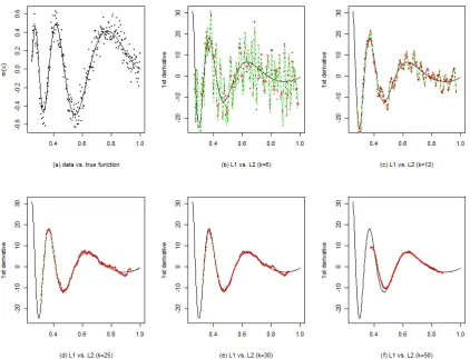
∼ N(0,0.12) and is plotted in Figure 1(a). Figure 1 (2) displays the LowLAD
(RLowLAD) estimator (use the R package ‘L1pack’ in Osorio (2015)) and the LowLSR estimator with k ∈ {6,12,25,30,50}. When k is small (see Figure 1(b) and 1(c)), both estimators are noise-corrupted versions of the true first-order derivatives; as k becomes larger (see Figure 1(d)-(f)), our estimator provides a similar performance as the LowLSR estimator. Furthermore, by combining the left part of Figure 1(d), the middle part of 1(e) and the right part of 1(f), more accurate derivative estimators can be obtained for practical use.
In addition, note that the three estimators have the same variation trend, whereas the LowLAD estimator has a slightly large oscillation and the RLowLAD estimator has a similar performance compared to the LowLSR estimator. These simulation results coincide with the theoretical results: the three estimators have the same bias, which explains the same variation trend; the variance ratios are Var( ˆm(1)LowLSR)/Var( ˆm(1)LowLAD) ≈ 0.64 and Var( ˆm(1)LowLSR)/Var( ˆm(1)RLowLAD)≈0.95, which explains the oscillation performance.
Next, we consider the non-normal errors: 90% of the errors come from∼N(0, σ2) with σ= 0.1, and the remaining 10% come from∼N(0, σ02) withσ0= 1 or 10 corresponding to the low or high contamination level. Figures 3 and 4 present the finite-sample performance of the first-order derivative estimators for the regression functionsm1 andm2, respectively. They show that the estimated curves of the first-order derivative based on LowLAD fit the true curves more accurately than LowLSR in the presence of heavy-tailed errors. The heavier the tail, the more significant the improvement.
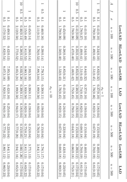
We also compute the mean absolute errors to further assess the performance of the four methods, i.e., LowLAD, RLowLAD, LowLSR and LAD. Since the oscillation of a periodic function depends on its frequency and amplitude, we consider the sine function in the following form as the regression function,
m3(x) =Asin(2πf x), x∈[0,1].
The errors are generated in the above contaminated way. We consider two sample sizes:
n = 100 and 500, two standard deviations: σ = 0.1 and 0.5, two contaminated standard deviations: σ0 = 1 and 10, two frequencies: f = 0.5 and 1, and two amplitudes: A= 1 and 10.
We use the following adjusted mean absolute error (AMAE) as the criterion of perfor-mance evalution:
AMAE(k) = 1
n−2k
n−k X
i=k+1
Figure 1: The comparison between the LowLAD and LowLSR estimators. (a) Simulated
data set of size 300 from model (1) with equidistantxi∈[0.25,1],i iid∼N(0,0.12),
and the true regression function m0(x) (bold line). (b)-(f) The first-order LowLAD derivative estimators (green points) and the first-order LowLSR deriva-tive estimators (red dashed line) for k∈ {6,9,12,25,30,50}. As a reference, the true first-order derivative fucntion is also plotted (bold line).
Due to the heavy computation (for example, it needs more than 48 hours for the case
n = 500 and k = n/5 = 100 based on 1000 repetitions on our personal computer), we choose k=n/5 uniformly.
Figure 2: The comparison between the RLowLAD and LowLSR estimators for the same data set as in Figure 1
6.2. Second-Order Derivative Estimators
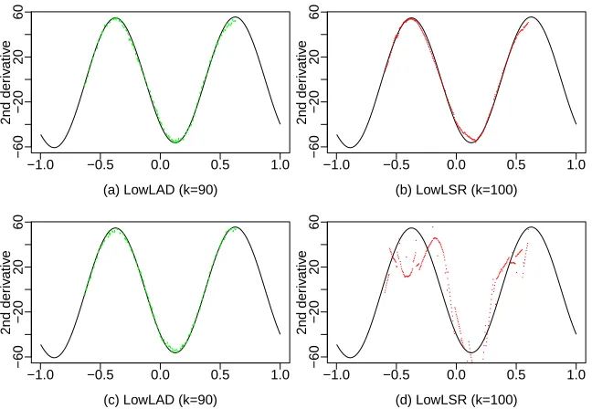
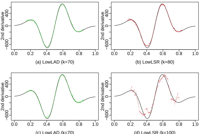
To assess the finite-sample performance of the second-order derivative estimators, we con-sider the same regression functions as in Section 6.1. Figures 5 and 6 present the estimated curves of the second-order derivatives ofm1andm2, respectively. It shows that our LowLAD estimator fits the true curves more accurately than the LowLSR estimator in all settings.
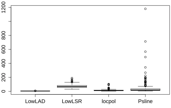
We further compare LowLAD with two other well-known methods: the local polyno-mial regression with p = 5 (use R package ‘locpol’ in Cabrera (2012)) and the penalized smoothing splines with norder = 6 and method = 4 (use R package ‘pspline’ in Ramsay and Ripley (2013)). For simplicity, we consider the simple version of m3 with A = 5 and
f = 1:
m4(x) = 5 sin(2πx), x∈[0,1].
−1.0 −0.5 0.0 0.5 1.0
−5
0
5
10
(a) LowLAD (k=70)
1st der
iv
ativ
e
−1.0 −0.5 0.0 0.5 1.0
−5
0
5
10
(b) LowLSR (k=70)
1st der
iv
ativ
e
−1.0 −0.5 0.0 0.5 1.0
−5
0
5
10
(c) LowLAD (k=70)
1st der
iv
ativ
e
−1.0 −0.5 0.0 0.5 1.0
−5
0
5
10
(d) LowLSR (k=100)
1st der
iv
ativ
e
Figure 3: (a-b) The true first-order derivative function (bold line), LowLAD (green line) and LowLSR estimators (red line). Model (1) with equidistantxi ∈[−1,1], regression functionm1, and∼90%N(0,0.12) + 10%N(0,12). (c-d) The same designs as in
(a-b) except∼90%N(0,0.12) + 10%N(0,102).
−1.0 −0.5 0.0 0.5 1.0
−60
−20
20
60
(a) LowLAD (k=90)
2nd der
iv
ativ
e
−1.0 −0.5 0.0 0.5 1.0
−60
−20
20
60
(b) LowLSR (k=100)
2nd der
iv
ativ
e
−1.0 −0.5 0.0 0.5 1.0
−60
−20
20
60
(c) LowLAD (k=90)
2nd der
iv
ativ
e
−1.0 −0.5 0.0 0.5 1.0
−60
−20
20
60
(d) LowLSR (k=100)
2nd der
iv
ativ
e
robust estimator is superior to the existing methods in the presence of sharp-peak and heavy-tailed errors.
6.3. House Price of China in Latest Ten Years
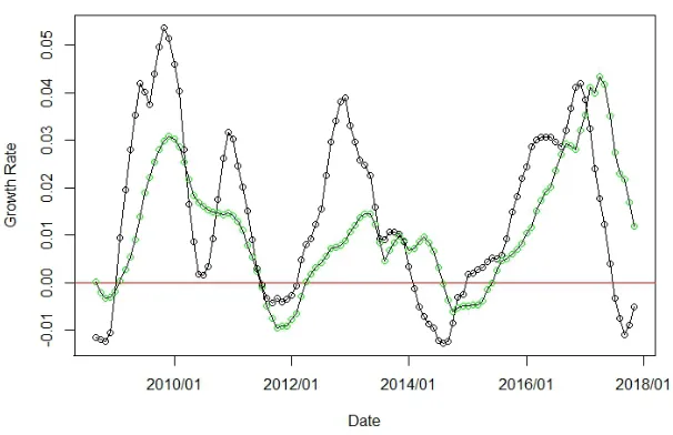
In reality, there are many data sets recorded by year, month, week, day, hour, minute, etc. For example, human growth is usually recorded by year, and temperature is recorded by hour, day or month. In this section, we apply RLowLAD to the data set of house price in two cities of China, i.e., Beijing and Jinan. We collect these monthly data from the web: http://www.creprice.cn/ (see Figure 9), which last from January 2008 to July 2018 and have size 127. We analyze this date set in two steps. Firstly, we apply our method to estimate the first-order derivative with k= 8 for RLowLAD and k = 6 for lower-order RLowLAD, where the lower-order means that we conduct the Taylor expansion to order 2 instead of order 4. Secondly, we define the relative growth rate as the ratio between the RLowLAD estimator and the house price at the same month, and then plot the relative growth rates in Figures 10 and 11. In the last ten years, the house price goes through tricycle fast increasing, and the monthly growth rate is larger than 0 most of the time with the maximum value at about 0.05.
7. Conclusion and Extensions
In this paper, we propose a robust differenced method for estimating the first- and higher-order derivatives of the regression function in nonparametric models. The new method consists of two main steps: first construct a sequence of symmetric difference quotients, and second estimate the derivatives using the LowLAD regression. The main contributions are as follows:
(1) Unlike LAD, our proposed LowLAD has the unique property of double robustness (or robustness2. Specifically, it is robust not only to heavy-tailed error distributions (like LAD), but also to low density of the error term at a specific quantile (LAD needs a high value of the error density at median; otherwise, the relative efficiency of LAD can be arbitrarily small compared with LowLAD). Following Theorem 1, the asymp-totic variance of the LowLAD estimator includes the term g(0) = 2R−∞∞ f2(x)dx = 2R−∞∞ f(F−1(τ))dτ, which implies that we are able to utilize the information of the whole error density. While for the LAD estimator, its variance depends on a single value f(0) only. In this sense, the LowLAD estimator is more robust than the LAD estimator.
(2) Our proposed LowLAD does not require the error distribution to have a zero median, and so is more flexible than LAD. To be more specific, our symmetric differenced errors are guaranteed to have a zero median and a positive symmetric density in a neighborhood of zero, regardless of whether or not the distribution of the original error is symmetric. While for LAD, we must require the error distribution to have a zero median, and consequently, the practical usefulness of LAD will be rather limited.
regres-sion (CQR) estimator. In other words, running one RLowLAD regression is equivalent to combining infinitely many quantile regressions.
(4) Lastly, it is also worthwhile to mention that the differences between LowLAD and LAD are strikingly distinct from the differences between LowLSR and LS. For the same data and the same tuning parameter k, we have LS = LowLSR, whereas LAD 6= LowLAD. What is more, RLowLAD is able to further improve the estimation efficiency compared with LowLAD, while RLowLSR, the LS counterpart of RLowLAD, is not able to improve efficiency relative to LowLSR.
LowLAD is a new idea to explore the information of density function by combining first-order difference and LAD. We can adopt the third-order symmetric difference{(Yi+j−
Yi−j) + (Yi+l−Yi−l)}or the third-order random difference{(Yi+j+Yi+l)−(Yi+u+Yi+v)}, even higher-order difference, to explore the information of density function. Whether and how to achieve the Cramer-Rao Lower bound deserves further study. These questions would be investigated in a separate paper.
In this paper, we focus on the derivative estimation with fixed designs and iid errors. With minor technical extensions, the proposed method can be extended to random designs with heteroskedastic errors. Further extensions to linear model, high-dimensional model for variable selection, semiparametric model, and change-point detection are also possible.
Acknowledgements
Appendix A. Proof of Theorem 1
Proposition 11 If i are iid with a continuous, positive densityf(·) in a neighborhood of the median, then ζ˜ij = (i+j−i−j)/2 (j=1,. . . , k) are iid with median0 and a continuous, positive, symmetric density g(·), where
g(x) = 2
Z ∞ −∞
f(2x+)f()d.
Proof of Proposition 11The distribution of ˜ζij = (i+j−i−j)/2 is
Fζ˜ij(x) =P((i+j −i−j)/2≤x) =
Z Z
i+j≤2x+i−j
f(i+j)f(i−j)di+jdi−j
=
Z ∞ −∞
{
Z 2x+i−j
−∞
f(i+j)di+j}f(i−j)di−j
=
Z ∞ −∞
F(2x+i−j)f(i−j)di−j.
Then the density of ˜ζij is
g(x),
dFζ˜ij(x) dx = 2
Z ∞ −∞
f(2x+i−j)f(i−j)di−j.
The densityg(·) is symmetric due to
g(−x) = 2
Z ∞ −∞
f(−2x+i−j)f(i−j)di−j
= 2
Z ∞ −∞
f(i−j)f(i−j+ 2x)di−j
=g(x).
Therefore, we have
Fζ˜
ij(0) =
Z ∞ −∞
F(i−j)f(i−j)di−j = 1 2F
2(
i−j)|∞−∞= 1 2,
g(0) = 2
Z ∞ −∞
f2(i−j)di−j.
Proof of Theorem 1Rewrite the objective function as
Sn(b) = 1
n
X
j
fn
˜
Yij|b
where
fn
˜
Yij|b = ˜
Yij(1)−bi1dj−bi3d3j
1
h1(0< dj ≤h)
with b= (bi1, bi3)T and h =k/n. Define Xj =
dj, d3j T
and H =diag
h, h3 . Note that arg min
b Sn(b) = arg minb [Sn(b)−Sn(β)], whereβ = m (1)(x
i), m(3)(xi)/6 T
.
We first show that H
b
β−β
= op(1), where βb = ( ˆβi1,βˆi3)T. We use Lemma 4 of
Porter and Yu (2015) to show the consistency. Essentially, we need to show that
(i) sup b∈B
|Sn(b)−Sn(β)−E [Sn(b)−Sn(β)]|
p
−→0,
(ii) inf
kH(b−β)k>δE [Sn(b)−Sn(β)]> εforn large enough, whereB is a compact parameter space forβ, andδ and εare fixed positive small numbers.
We use Lemma 2.8 of Pakes and Pollard (1989) to show (i), where
Fn=nfn
˜
Y|b−fn
˜
Y|β:b∈ Bo.
Note that Fn is Euclidean (see, e.g., Definition 2.7 of Pakes and Pollard (1989) for the definiton of an Euclidean-class of functions) by applying Lemma 2.13 of Pakes and Pollard (1989), where α = 1, f(·, t0) = 0, φ(·) =kXjkh11(0< dj ≤h) and the envelope function is Fn(·) = M φ(·) for some finite constant M. Since E [Fn] = E
kXjk1h1(0< dj ≤h)
=
O(h)<∞, Lemma 2.8 of Pakes and Pollard (1989) implies
sup b∈B
|Sn(b)−Sn(β)−E[Sn(b)−Sn(β)]|
p
−→0.
As to inf
kH(b−β)k>δE[Sn(b)−Sn(β)], by Proposition 1 of Wang and Scott (1994), E [Sn(b)−Sn(β)]
.
=1
n
X
j
g(0)XjTH−1H(b−β)2 1
h1(0< dj ≤h)
−1
n
X
j 2g(0)
m(di+j)−m(di−j)
2 −X
T j β
XjTH−1H(b−β)1
h1(0< dj ≤h)
&δ2−h5δ,
where = means that the higher-order terms are omitted, and. & means the left side is bounded blow by a constant times the right side.
We then derive the asymptotic distribution of√nhH
b
β−β
by applying the empirical process technique. First, the first order conditions can be written as
1 n X j sign ˜
Yij(1)−ZjTHβb
Zj
√ h
which is denoted as
1
n
X
j
fn0( ˜Yij(1)|βb),Sn0
b
β=op(1),
whereZj =H−1Xj. By Example 2.9 of Pakes and Pollard (1989),Fn0 forms an Euclidean-class of functions with envelopeFn0 =kZjk
√ h
h 1(0< dj ≤h), whereF 0 n=
n
fn0( ˜Yij(1)|b) :b∈ Bo, and E
Fn02
<∞. So by Lemma 2.17 of Pakes and Pollard (1989) andHβb−β
=op(1),
Gn
fn0( ˜Yij(1)|βb)
=Gn
fn0( ˜Yij(1)|β)+op(1), whereGn(f) =
√
n(Pn−P)f is the standardized empirical process, andPnis the empirical measure of the original data. Since
√ nX j E h
fn0( ˜Yij(1)|βb) i
−E
h
fn0( ˜Yij(1)|β)
i .
=−√nh2g(0) nh
X
j
ZjZjTH
b
β−β
, and 1 nh X j
signY˜ij(1)−ZjTHβZj1(0< dj ≤h)
− 1 nh X j sign ˜
Yij(1)−m(di+j)−m(di−j)
2
Zj1(0< dj ≤h)=. 2g(0)
nh
X
j
Zjd5j
m(5)(xi) 5! , we have √ nh H b
β−β−
1 nh X j
ZjZjT −1 1 nh X j
Zjd5j
m(5)(xi) 5!
.
= 1 2g(0)
1 nh X j
ZjZjT −1 1 √ nh X j sign ˜
ζij(1)
Zj1(0< dj ≤h).
In other words,
2g(0)Vk
bβ−β−Vk−2 k X
j=1
Xjd5j
m(5)(xi) 5!
.
=Vk−1
k X
j=1
signζ˜ij(1)Xj,
where Vk = (Pkj=1XjXjT)1/2 is a symmetric positive definite matrix. By Cram´er-Wold device and Lyapunov CLT, we complete the proof of asymptotic normality.
The bias of ˆβi1 is
Bias[ ˆβi1]= [1. ,0]
X
j
XjXjT −1 k X j=1
Xjd5j
m(5)(xi) 5! =−
m(5)(xi) 504
and the variance is
Var[ ˆβi1]=. 1
4g(0)2[1,0]
X
j
XjXjT
−1
1 0
≈ 75
16g(0)2
n2
k3. Combining the squared bias and the variance, we obtain the AMSE
AMSE[ ˆβi1] =
m(5)(xi)2 5042
k8 n8 +
75 16g(0)2
n2
k3. (17)
To minimize (17) with respect tok, we take the first-order derivative of (17) and yield the gradient as
dAMSE[ ˆβi1] dk =
m(5)(xi)2 31752
k7 n8 −
225 16g(0)2
n2 k4. Our optimization problem is to solve dAMSE[ ˆβi1]
dk = 0. So we obtain
kopt =
893025 2g(0)2m(5)(x
i)2 1/11
n10/11≈3.26
1
g(0)2m(5)(x i)2
1/11
n10/11,
and
AMSE[ ˆβi1]≈0.19(m(5)(xi)6/g(0)16)1/11n−8/11. Appendix B. Proof of Theorem 2
Rewrite the objective function as a U-process,
Sn(b) = X
l<j
fn(Yi+j, Yi+l|b),
where
fn(Yi+j, Yi+l|b) =
Yi+j−Yi+l−b1(dj−dl)−bi2(d2j−dl2)−b3(d3j−d3l)−b4(d4j −d4l)
· 1
h21(0<|dj| ≤h)1(0<|dl| ≤h)
with b= (bi1, bi2, bi3, bi4)T and h=k/n. DefineUn= n(n−1)2 Sn(b),H =diag
h, h2, h3, h4
and Xjl=
dj −dl, d2j −d2l, d3j−d3l, d4j −d4l T
. Note that arg min
b Sn(b) = arg minb Un(b) = arg min
b [Un(b)−Un(β)], where β= m (1)(x
i), m(2)(xi)/2!, m(3)(xi)/3!, m(4)(xi)/4! T
.
We first show thatH
b
β−β
=op(1), whereβb= ( ˆβi1RLowLAD,βˆi2RLowLAD,βˆi3RLowLAD,βˆi4RLowLAD)T.
We use Lemma 4 of Porter and Yu (2015) to show the consistency. Essentially, we need to show that
(i) sup b∈B
|Un(b)−Un(β)−E [Un(b)−Un(β)]|
p
(ii) inf
kH(b−β)k>δE [Un(b)−Un(β)]> εfornlarge enough, where Bis a compact parameter space forβ, andδ and εare fixed positive small numbers.
We use Theorem A.2 of Ghosal et al. (2000) to show (i), where
Fn={fn(Yi+j, Yi+l|b)−fn(Yi+j, Yi+l|β) :b∈ B}.
Note thatFn forms an Euclidean-class of functions by applying Lemma 2.13 of Pakes and Pollard (1989), where α = 1, f(·, t0) = 0, φ(·) = kXjlkh121(|dj| ≤ h)1(|dl| ≤ h) and the envelope function is Fn(·) =M φ(·) for some finite constant M. It follows that
NεkFnkQ,2,Fn, L2(Q)
.ε−C
for any probability measure Qand some positive constant C, where. means the left side is bounded by a constant times the right side. Hence,
1
nE
Z ∞
0
logN(ε,Fn, L2(U2n))dε
. 1
n
p
E [F2 n]
Z ∞ 0
log1
εdε=O
1
n
,
where U2n is the random discrete measure putting mass n(n−1)1 on each of the points (Yi+j, Yi+l). Next, by Lemma A.2 of Ghosal et al. (2000), the projections
fn(Yi+j|b) = Z
fn(Yi+j, Yi+l|b)dFYi+l(Yi+l)
satisfy
sup Q
NεFn
Q,2,Fn, L2(Q)
.ε−2C,
whereFn=
fn(Yi+j|b)−fn(Yi+j|β) :b∈ B , and Fn is an envelope ofFn. Thus
1
√ nE
Z ∞
0
logN ε,Fn, L2(Pn)
dε
. √1
n
r
E
h
F2n
iZ ∞ 0
log1
εdε=O
1
√ n
.
By Theorem A.2 and Markov’s inequality, sup b∈B
|Un(b)−Un(β)−E [Un(b)−Un(β)]|
p
−→0.
As to inf
kH(b−β)k>δE[Un(b)−Un(β)], by Proposition 1 of Wang and Scott (1994), E [Un(b)−Un(β)]
.
= 2
n(n−1)
X
l<j
g(0) 2
XjlTH−1H(b−β)2 1
h21(0<|dj| ≤h)1(0<|dl| ≤h)
− 2
n(n−1)
X
l<j
g(0)m(di+j)−m(di+l)−XjlTβ XjlTH −1
H(b−β)
1
h21(0<|dj| ≤h)1(0<|dl| ≤h)
We then derive the asymptotic distribution of √nhH
b
β−β
. First, by Theorem A.1 of Ghosal et al. (2000), we approximate the first order conditions by an empirical process.
Second, we derive the asymptotic distribution of√nhH
b
β−β
by applying the empirical process technique.
First, the first order conditions can be written as
2
n(n−1)
X
l<j
signYi+j−Yi+l−ZjlTHβb
Zjl
√ h
h2 1(0<|dj| ≤h)1(0<|dl| ≤h) =op(1), which is denoted as
2
n(n−1)
X
l<j
fn0(Yi+j, Yi+l|βb),
2
n(n−1)S 0 n
b
β=op(1),
whereZjl=H−1Xjl. By Example 2.9 of Pakes and Pollard (1989),Fn0 forms an Euclidean-class of functions with envelopeFn0 =kZjlk
√ h
h21(|dj| ≤h)1(|dl| ≤h), where
Fn0 =
fn0(Yi+j, Yi+l|b) :b∈ B ,
so
NεFn0
Q,2,F 0
n, L2(Q)
.ε−V
for any probability measure Q and some positive constant V. By Theorem A.1 and the discussion following Theorem A.1 and A.2 in Ghosal et al. (2000), it follows that
nE
"
sup f0
n∈Fn0
U2nfn0 −2Pn
E2
fn0(Yi+j, Yi+l|b)
−E
fn0(Yi+j, Yi+l|b) # .E Z ∞ 0
logN ε,Fn0, L2(U2n) dε . Z 1 0
log ε−Vdε
r
E
h
(Fn0)2
i
.h−1/2,
whereE2[·] takes expectation onYi+l and also averages overdl, andE[·] takes expectation on (Yi+j, Yi+l) and also averages over (dj, dl). As a result,
√ n sup
f0 n∈Fn0
U2nfn0 −2Pn
E2[·]
fn0(Yi+j, Yi+l|b)
+E
fn0(Yi+j, Yi+l|b)
=op(1),
which implies
√ n2Pn
h
E2 h
fn0(Yi+j, Yi+l|βb) ii
−Ehfn0(Yi+j, Yi+l|βb)
i
=op(1),
where
E2
fn0(Yi+j, Yi+l|b) = √ h nh2 X l
2F Yi+j−m(di+l)−ZjlTHb
−1
withF(·) being the cumulative distribution function of . In other words,
2Gn
E2 h
fn0(Yi+j, Yi+l|βb) i
+√nEhfn0(Yi+j, Yi+l|βb) i
=op(1).
By Lemma 2.13 of Pakes and Pollard (1989), F0 1n =
E2[fn0(Yi+j, Yi+l|b)] :b∈ B is Eu-clidean with envelopeF1n=
√ h nh2
P l
kZjlk1(0<|dj| ≤h)1(0<|dl| ≤h), so by Lemma 2.17
of Pakes and Pollard (1989) and Hβb−β
=op(1),
Gn
E2 h
fn0(Yi+j, Yi+l|βb) i
=Gn E2
fn0(Yi+j, Yi+l|β)
+op(1).
As a result,
2Gn E2
fn0(Yi+j, Yi+l|β)
+√nE
h
fn0(Yi+j, Yi+l|βb) i
=2√nPn E2
fn0(Yi+j, Yi+l|β)
−2√nEfn0(Yi+j, Yi+l|β)
+√n
E
h
fn0(Yi+j, Yi+l|βb) i
−Efn0(Yi+j, Yi+l|β)
+√nEfn0(Yi+j, Yi+l|β)
=2√nPnE2
fn0(Yi+j, Yi+l)
+ 2√nPn E2
fn0(Yi+j, Yi+l|β)
−E2
fn0(Yi+j, Yi+l)
+√nEhfn0(Yi+j, Yi+l|βb) i
−E
fn0(Yi+j, Yi+l|β)
−√nE
fn0(Yi+j, Yi+l|β)
=2√nPnE2
fn0(Yi+j, Yi+l)
+√n
E
h
fn0(Yi+j, Yi+l|βb) i
−Efn0(Yi+j, Yi+l|β)
+√nEfn0(Yi+j, Yi+l|β)
=op(1), where
E2
fn0(Yi+j, Yi+l) = √ h nh2 X l
[2F(i+j)−1]Zjl1(0<|dj| ≤h)1(0<|dl| ≤h)
satisfiesEE2[fn0(Yi+j, Yi+l)]
= 0, and the second to last equality is from
√
nPn E2
fn0(Yi+j, Yi+l|β)
−E2
fn0(Yi+j, Yi+l) .
=√nEfn0(Yi+j, Yi+l|β)
.
Since
Efn0(Yi+j, Yi+l|b)
=
√ h n2h2
X
l,j
Zjl1(0<|dj| ≤h)1(0<|dl| ≤h)
·
2
Z
F +m(di+j)−m(di+l)−ZjlTHb
−1
f()d,
we have √ n E h
fn0(Yi+j, Yi+l|βb) i
−Efn0(Yi+j, Yi+l|β)
.
=−√nhg(0)
1
n2h2 X
l,j
ZjlZjlT
H
b
β−β
,
√
nEfn0(Yi+j, Yi+l|β) .
=
√
nhg(0) 1
n2h2 X
l,j
Zjl d5j −d5l
m(5)(xi)
In summary, √ nh H b
β−β
−
1
n2h2 X
l,j
ZjlZjlT
−1
1
n2h2 X
l,j
Zjl d5j −d5l
m(5)(xi) 5!
.
=2g(0)−1
1
n2h2 X
l,j
ZjlZjlT
−1
√ nPnE2
fn0(Yi+j, Yi+l)
,
Thus, the asymptotic bias is
eTH−1
1
n2h2 X
l,j
ZjlZjlT
−1
1
n2h2 X
l,j
Zjl d5j −d5l
m(5)(xi) 5! =−
m(5)(xi) 504
k4 n4, and the asymptotic variance is
4
kg(0)2e
TH−1G−1V G−1H−1e= 75 24g(0)2
n2 k3, wheree= (1,0,0,0)T,G= k12
P
l,jZjlZjlT, andV = 3k1 Pk
j=−k(1k Pk
l=−kZjl)(k1 Pk
l=−kZjl)T with Var (2F(i+j)−1) = 1/3.
Appendix C. Proof of Theorem 9
Proof of Theorem 9Following the proof of Theorem 1, the leading term of the bias is
Bias[ ˆβi11] =
m(2)(xi) 2
k4+ 2k3i−2ki3−i3 n(k3+ 3k2i+ 3ki2+i3), and the leading term of the variance is
Var[ ˆβi11] = 3
f(0)2
n2
k3+ 3k2i+ 3ki2+i3.
Appendix D. Proof of Theorem 10
Proposition 12 If the errors i are iid with a symmetric (about 0), continuous, positive density function f(·), then δ˜ij =i+j+i−j (j=1, . . . , k) are iid with M edian[˜δij] = 0 and a continuous, positive density h(·) in a neighborhood of 0, where
h(x) =
Z ∞ −∞
Proof of Proposition 12The distribution of ˜δij =i+j+i−j is
Fδ˜ij(x) =P(i+j+i−j ≤x) =
Z Z
i+j≤x−i−j
f(i+j)f(i−j)di+jdi−j
=
Z ∞ −∞
{
Z x−i−j
−∞
f(i+j)di+j}f(i−j)di−j
=
Z ∞ −∞
F(x−i−j)f(i−j)di−j.
Then the density of ˜δij is
h(x), dF˜δij(x)
dx =
Z ∞ −∞
f(x−i−j)f(i−j)di−j.
By the symmetry of the density function, we have
Fδ˜ij(0) = Z ∞
−∞
F(−i−j)f(i−j)di−j
=
Z ∞ −∞
(1−F(i−j))f(i−j)di−j
=(F −1
2F 2(
i−j))|∞−∞ =1
2,
h(0) =
Z ∞ −∞
f2(i−j)di−j.
Proof of Theorem 10 Following the proof of Theorem 1, the asymptotic bias is
Bias[ ˆαi2] =−
m(6)(xi) 792
k4 n4 +o
k4 n4
,
and the asymptotic variance of ˆαi1 is
Var[ ˆαi2] = 2205 64h(0)2
n4 k5 +o
n4 k5
.
Combining the squared bias and the variance, we obtain the AMSE as
AMSE[ ˆαi2] =
m(6)(xi)2 7922
k8 n8 +
2205 64h(0)2
n4
To minimize (18) with respect tok, we take the first-order derivative of (18) and yield the gradient as
dAMSE[ ˆαi2] dk =
m(6)(xi)2 78408
k7 n8 −
11025 16h(0)2
n4 k6. Now the optimization problem is to solve dAMSE[ ˆαi2]
dk = 0. So we obtain
kopt =
108056025 8h(0)2m(6)(x
i)2 1/13
n12/13≈3.54
1
h(0)2m(6)(x i)2
1/13
n12/13,
and
AMSE[ ˆαi2]≈0.29(m(6)(xi)10/h(0)16)1/13n−8/13.
Appendix E. Variance Ratios for Popular Distributions
Variance Ratios for Eight Error Distributions
In this subsection, we investigate the variance ratio of the RLowLAD estimator with respect to the LowLSR and LAD estimators for eight error distributions.
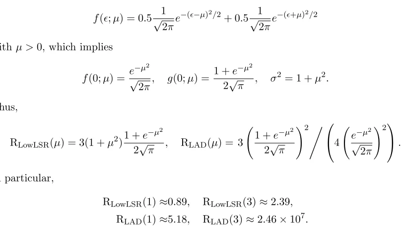
From the main text,
RLowLSR(f) = 3σ2g(0)2, RLAD(f) = 3g(0)2 4f(0)2.
Example 1: Normal distribution. The error density function is f() = √1
2πexp(− 2/2), which implies
f(0) = √1
2π, g(0) = 2
Z ∞ −∞
1 2πe
−2
d= √1 π.
Due toσ2 = 1, we have
RLowLSR(f) = 3/π≈0.95, RLAD(f) = 1.50.
In other words, the RLowLAD estimator is almost as efficient as the LowLSR estimator for the normal distribution.
Example 2: Mixed normal distribution. The error density function is
f(;α, σ0) = (1−α) 1
√
2πe
−2/2
+α√ 1
2πσ0
with 0< α≤1/2 andσ0>1, which implies
f(0;α, σ0) =(1−α) 1
√
2π +α
1
√
2πσ0
,
g(0;α, σ0) =2 Z ∞
−∞
f2()d
=2
(
(1−α)2
Z ∞ −∞
1 2πe
−2
d+ 2α(1−α)
Z ∞ −∞
1 2πσ0
e−(
2
2+
2
2σ2
1
) d
+α2
Z ∞ −∞
1 2πσ02e
−x2 σ2
0d
)
=2
(
(1−α)2 1
2√π + 2α(1−α)
1
√
2πp1 +σ2 0
+α2 1
2√πσ0 )
,
Var(i) =(1−α) +ασ20 ,σ2. Thus,
RLowLSR(α, σ0) =12
(1−α) +ασ02
(
(1−α)2 1
2√π + 2α(1−α)
1
√
2πp1 +σ02 +α
2 1
2√πσ0 )2
,
RLAD(α, σ0) = 3
(1−α)2 1
2√π + 2α(1−α) 1 √
2π√1+σ2 0
+α2 1 2√πσ0
2 n
(1−α)√1 2π +α
1 √
2πσ0
o2 .
In particular,
RLowLSR(0.1,3)≈1.80, RLowLSR(0.1,10)≈10.90, RLAD(0.1,3)≈1.38, RLAD(0.1,10)≈1.27. Example 3: t distribution. The error density function is
f(;ν) = Γ((√ν+ 1)/2) νπΓ(ν/2)
1 + 2
ν
−(ν+1)/2)
with the degree of freedomν >2, which implies
f(0) =Γ((√ν+ 1)/2) νπΓ(ν/2) ,
g(0) =2
Z ∞ −∞
1
νπ
Γ((ν+ 1)/2) Γ(ν/2)
2
1 + 2
ν
−(ν+1)
d= √2 νπ
Γ((ν+ 1)/2) Γ(ν/2)
2
Γ(ν+ 1/2) Γ(ν+ 1) . Due toσ2 =ν/(ν−2), we have
RLowLSR(ν) = 12 (ν−2)π
Γ((ν+ 1)/2) Γ(ν/2)
4
Γ(ν+ 1/2) Γ(ν+ 1)
2
,
RLAD(ν) =3
Γ((ν+ 1)/2) Γ(ν/2)
2
Γ(ν+ 1/2) Γ(ν+ 1)
2
Forν = 3,
RLowLSR(3) = 75/(4π2)≈1.90, RLAD(3) = 75/64≈1.17.
Example 4: Laplace (double exponential) distribution. The error density function is
f() = 12exp(−||), which implies
f(0) = 1
2, g(0) = 2
Z ∞ −∞
1 4e
−2|| d= 1
2.
Due toσ2 = 2, we have
RLowLSR(f) = 1.50, RLAD(f) = 0.75.
Example 5: Logistic distribution. The error density function isf() = exp()/(exp() + 1)2, which implies
f(0) = 1
4, g(0) = 2
Z ∞ −∞
e2
(exp() + 1)4d= 1 3.
Due toσ2 =π2/3, we have
RLowLSR(f) =π2/9≈1.10, RLAD(f) = 4/3≈1.33.
Example 6: Cauchy distribution. The error density function is f() = 1/(π(1 +2)), which implies
f(0) = 1
π, g(0) =
1
π, Var() =∞.
Thus,
RLowLSR(f) =∞, RLAD(f) = 0.75.
Example 7: Mixed double Gamma distribution. The error density function is
f(;α, k) = (1−α)1 2e
−||
+α 1
2Γ(k+ 1)|| ke−||
with parameter k >0 and the mixed ratio α, which implies
f(0;α, k) =1−α 2 +
α
2Γ(k+ 1),
g(0;α, k) =2
Z ∞ −∞
f2(;α, k)d
=
Z ∞ −∞
(1−α)2 2 e
−2||
+(1−α)α Γ(k+ 1)||
ke−2||
+ α
2 2Γ(k+ 1)2||
2ke−2|| d
=(1−α) 2
2 +
α(1−α) 2k +
![Figure 1: The comparison between the LowLAD and LowLSR estimators. (a) Simulateddata set of size 300 from model (1) with equidistant xi ∈ [0.25, 1], ϵiiid∼ N(0, 0.12),and the true regression function m0(x) (bold line).(b)-(f) The first-orderLowLAD derivativ](https://thumb-us.123doks.com/thumbv2/123dok_us/9770761.1962259/18.612.91.513.112.434/comparison-estimators-simulateddata-equidistant-regression-function-orderlowlad-derivativ.webp)