Measuring the Effects of Data Parallelism on Neural Network Training

(1)

Measuring the Effects of Data Parallelism

on Neural Network Training

Christopher J. Shallue∗ [email protected]

Jaehoon Lee∗ † [email protected]

Joseph Antognini† [email protected]

Jascha Sohl-Dickstein [email protected]

Roy Frostig [email protected]

George E. Dahl [email protected]

Google Brain

1600 Amphiteatre Parkway Mountain View, CA, 94043, USA

Editor:Rob Fergus

Abstract

Recent hardware developments have dramatically increased the scale of data parallelism available for neural network training. Among the simplest ways to harness next-generation hardware is to increase the batch size in standard mini-batch neural network training al-gorithms. In this work, we aim to experimentally characterize the effects of increasing the batch size on training time, as measured by the number of steps necessary to reach a goal out-of-sample error. We study how this relationship varies with the training algorithm, model, and data set, and find extremely large variation between workloads. Along the way, we show that disagreements in the literature on how batch size affects model quality can largely be explained by differences in metaparameter tuning and compute budgets at different batch sizes. We find no evidence that larger batch sizes degrade out-of-sample performance. Finally, we discuss the implications of our results on efforts to train neu-ral networks much faster in the future. Our experimental data is publicly available as a database of 71,638,836 loss measurements taken over the course of training for 168,160 individual models across 35 workloads.

Keywords: neural networks, stochastic gradient descent, data parallelism, batch size, deep learning

1. Introduction

Neural networks have become highly effective at a wide variety of prediction tasks, in-cluding image classification, machine translation, and speech recognition. The dramatic improvements in predictive performance over the past decade have partly been driven by advances in hardware for neural network training, which have enabled larger models to be trained on larger datasets than ever before. However, although modern GPUs and custom

∗. Both authors contributed equally.

†. Work done as a member of the Google AI Residency program (g.co/airesidency).

c

(2)

accelerators have made training neural networks orders of magnitude faster, training time still limits both the predictive performance of these techniques and how widely they can be applied. For many important problems, the best models are still improving at the end of training because practitioners cannot afford to wait until the performance saturates. In extreme cases, training must end before completing a single pass over the data (e.g. Anil et al., 2018). Techniques that speed up neural network training can significantly benefit many important application areas. Faster training can facilitate dramatic improvements in model quality by allowing practitioners to train on more data (Hestness et al., 2017), and by decreasing the experiment iteration time, allowing researchers to try new ideas and configurations more rapidly. Faster training can also allow neural networks to be deployed in settings where models have to be updated frequently, for instance when new models have to be produced when training data get added or removed.

Data parallelism is a straightforward and popular way to accelerate neural network training. For our purposes, data parallelism refers to distributing training examples across multiple processors to compute gradient updates (or higher-order derivative information) and then aggregating these locally computed updates. As long as the training objective decomposes into a sum over training examples, data parallelism is model-agnostic and ap-plicable to any neural network architecture. In contrast, the maximum degree of model parallelism (distributing parameters and computation across different processors for the same training examples) depends on the model size and structure. Although data paral-lelism can be simpler to implement, ultimately, large scale systems should consider all types of parallelism at their disposal. In this work, we focus on the costs and benefits of data parallelism in the synchronous training setting.

Hardware development is trending towards increasing capacity for data parallelism in neural network training. Specialized systems using GPUs or custom ASICs (e.g. Jouppi et al., 2017) combined with high-performance interconnect technology are unlocking un-precedented scales of data parallelism where the costs and benefits have not yet been well studied. On the one hand, if data parallelism can provide a significant speedup at the limits of today’s systems, we should build much bigger systems. On the other hand, if additional data parallelism comes with minimal benefits or significant costs, we might consider design-ing systems to maximize serial execution speed, exploit other types of parallelism, or even prioritize separate design goals such as power use or cost.

There is considerable debate in the literature about the costs and benefits of data paral-lelism in neural network training and several papers take seemingly contradictory positions. Some authors contend that large-scale data parallelism is harmful in a variety of ways, while others contend that it is beneficial. The range of conjectures, suggestive empirical results, and folk knowledge seems to cover most of the available hypothesis space. Answering these questions definitively has only recently become important (as increasing amounts of data parallelism have become practical), so it is perhaps unsurprising that the literature remains equivocal, especially in the absence of sufficiently comprehensive experimental data.

(3)

our methodology, and we discuss what we see as the most interesting unanswered questions that arise from our experiments.

1.1. Scope

We restrict our attention to variants of mini-batch stochastic gradient descent (SGD), which are the dominant algorithms for training neural networks. These algorithms iteratively update the model’s parameters using an estimate of the gradient of the training objective. The gradient is estimated at each step using a different subset, or(mini-) batch, of training examples. See Section 2.2 for a more detailed description of these algorithms. A data-parallel implementation computes gradients for different training examples in each batch in parallel, and so, in the context of mini-batch SGD and its variants, we equate the batch size with the amount of data parallelism.1 We restrict our attention to synchronous SGD because of its popularity and advantages over asynchronous SGD (Chen et al., 2016).

Practitioners are primarily concerned with out-of-sample error and the cost they pay to achieve that error. Cost can be measured in a variety of ways, including training time and hardware costs. Training time can be decomposed into number of steps multiplied by average time per step, and hardware cost into number of steps multiplied by average hardware cost per step. The per-step time and hardware costs depend on the practitioner’s hardware, but the number of training steps is hardware-agnostic and can be used to compute the total costs for any hardware given its per-step costs. Furthermore, in an idealized data-parallel system where the communication overhead between processors is negligible, training time depends only on the number of training steps (and not the batch size) because the time per step is independent of the number of examples processed. Indeed, this scenario is realistic today in systems like TPU pods2, where there are a range of batch sizes for which the time per step is almost constant. Since we are primarily concerned with training time, we focus on number of training steps as our main measure of training cost.

An alternative hardware-agnostic measure of training cost is the number of training examples processed, or equivalently the number of passes (epochs) over the training data. This measure is suitable when the per-step costs are proportional to the number of examples processed (e.g. hardware costs proportional to the number of floating point operations). However, the number of epochs is not a suitable measure of training time in a data-parallel system—it is possible to reduce training time by using a larger batch size and processing more epochs of training data, provided the number of training steps decreases.

In light of practitioners’ primary concerns of out-of-sample error and the resources needed to achieve it, we believe the following questions are the most important to study to understand the costs and benefits of data parallelism with mini-batch SGD and its variants:

1. What is the relationship between batch size and number of training steps to reach a goal out-of-sample error?

2. What governs this relationship?

3. Do large batch sizes incur a cost in out-of-sample error?

1. Mini-batch SGD can be implemented in a variety of ways, including data-serially, but a data-parallel implementation is always possible given appropriate hardware.

(4)

1.2. Contributions of This Work

1. We show that the relationship between batch size and number of training steps to reach a goal out-of-sample error has the same characteristic form across six different families of neural network, three training algorithms, and seven data sets.

Specifically, for each workload (model, training algorithm, and data set), increasing the batch size initially decreases the required number of training steps proportionally, but eventually there are diminishing returns until finally increasing the batch size no longer changes the required number of training steps. To the best of our knowledge, we are the first to experimentally validate this relationship across models, training algorithms, and data sets while independently tuning the learning rate, momentum, and learning rate schedule (where applicable) for each batch size. Unlike prior work that made strong assumptions about these metaparameters, our results reveal a uni-versal relationship that holds across all workloads we considered, across different error goals, and when considering either training error or out-of-sample error.

2. We show that the maximum useful batch size varies significantly between workloads and depends on properties of the model, training algorithm, and data set. Specifically, we show that:

(a) SGD with momentum (as well as Nesterov momentum) can make use of much larger batch sizes than plain SGD, suggesting future work to study the batch size scaling properties of other algorithms.

(b) Some models allow training to scale to much larger batch sizes than others. We include experimental data on the relationship between various model properties and the maximum useful batch size, demonstrating that the relationship is not as simple as one might hope from previous work (e.g. wider models do not always scale better to larger batch sizes).

(c) The effect of the data set on the maximum useful batch size tends to be smaller than the effects of the model and training algorithm, and does not depend on data set size in a consistent way.

3. We show that the optimal values of training metaparameters do not consistently follow any simple relationships with the batch size. In particular, popular learning rate heuristics—such as linearly scaling the learning rate with the batch size— do not hold across all problems or across all batch sizes.

(5)

1.3. Experimental Data

We release our raw experimental data for any further analysis by the research community.3 Our database contains 454 combinations of workload (model, data set, training algorithm) and batch size, each of which is associated with a metaparameter search space and a set of models trained with different configurations sampled from the search space. In total, our data contains 71,638,836 loss measurements taken over the course of training for 168,160 individual models. Together, these measurements make up the training curves of all of the individual models we trained, and can be used to reproduce all plots in this paper.4

2. Setup and Background

In this section we set up the basic definitions and background concepts used throughout the paper.

2.1. Learning

A data distribution is a probability distribution Dover a data domain Z. For example, we might consider a supervised learning task over a domain Z = X × Y, where X is the set of 32-by-32-pixel color images and Y is the set of possible labels denoting what appears in the image. A training set z1, . . . , zn∈ Z is a collection of examples from the data domain, conventionally assumed to be drawn i.i.d. from the data distribution D.

A machine learningmodel is a function that, givenparametersθfrom some set Θ⊂_Rd_, and given a data point z ∈ Z, produces a prediction whose quality is measured by a differentiable non-negative scalar-valued loss function.5 We denote by `(θ;z) the loss of a prediction made by the model, under parameters θ, on the data point z. We denote by L

theout-of-sample loss orexpected loss:

L(θ) = _E

z∼D[`(θ;z)], (1)

and by ˆLtheempirical average loss under a data set S= (z1, . . . , zn): ˆ

L(θ;S) = 1

n

n X

i=1

`(θ;zi). (2)

When S is the training set, we call ˆL theaverage training loss. We will say that the data sourceD, loss`, and model with parameter set Θ together specify a learningtask, in which our aim is to find parameters θ that achieve low out-of-sample loss (Equation 1), while given access only tontraining examples. A common approach is to find parameters of low average training loss (Equation 2) as an estimate of the out-of-sample loss (Shalev-Shwartz and Ben-David, 2014).

When minimizing average training loss ˆL, it is common to add regularization penalties to the objective function. For a differentiable penalty R : Θ → _R₊, regularization weight

3.https://github.com/google-research/google-research/tree/master/batch_science

4.https://colab.research.google.com/github/google-research/google-research/blob/master/

batch_science/reproduce_paper_plots.ipynb

(6)

λ >0, and training set S, the training objective might be

J(θ) = ˆL(θ;S) +λR(θ). (3)

In practice, we often approach a task by replacing its loss with another that is more amenable to training. For instance, in supervised classification, we might be tasked with learning under the 0/1 loss, which is an indicator of whether a prediction is correct (e.g. matches a ground-truth label), but we train by considering instead a surrogate loss (e.g. the logistic loss) that is more amenable to continuous optimization. When the surrogate loss bounds the original, achieving low loss under the surrogate implies low loss under the original. To distinguish the two, we say error to describe the original loss (e.g. 0/1), and we saveloss to refer to the surrogate used in training.

2.2. Algorithms

The dominant algorithms for training neural networks are based on mini-batch stochastic gradient descent (SGD, Robbins and Monro, 1951; Kiefer et al., 1952; Rumelhart et al., 1986; Bottou and Bousquet, 2008; LeCun et al., 2015). Given an initial point θ0 ∈ Θ, mini-batch SGD attempts to decrease the objective J via the sequence of iterates

θt←θt−1−ηtg(θt−1;Bt),

where eachBtis a random subset of training examples, the sequence{ηt}of positive scalars is called thelearning rate, and where, for any θ∈Θ andB ⊂S,

g(θ;B) = 1

|B|

X

z∈B

∇`(θ;z) +λ∇R(θ). (4)

When the examples B are a uniformly random subset of training examples, g(θ;B) forms an unbiased estimate of the gradient of the objective J that we call a stochastic gradient. In our larger-scale experiments, when we sample subsequent batchesBt, we actually follow the common practice of cycling through permutations of the training set (Shamir, 2016). The result of mini-batch SGD can be any of the iteratesθtfor which we estimate thatL(θt) is low using a validation data set.

Variants of SGD commonly used with neural networks include SGD with momentum (Polyak, 1964; Rumelhart et al., 1986; Sutskever et al., 2013), Nesterov momentum (Nes-terov, 1983; Sutskever et al., 2013), RMSProp (Hinton et al., 2012), and Adam (Kingma and Ba, 2015). All of these optimization procedures, or optimizers, interact with the training examples only by repeatedly computing stochastic gradients (Equation 4), so they support the same notion of batch size that we equate with the scale of data parallelism. In this work, we focus on the SGD, SGD with momentum, and Nesterov momentum optimizers. The latter two optimizers are configured by a learning rate{ηt}and a scalarγ ∈(0,1) that we callmomentum. They define the iterates6

SGD with momentum Nesterov momentum

vt+1←γvt+g(θt;Bt) vt+1←γvt+g(θt;Bt)

θt+1←θt−ηtvt+1 θt+1←θt−ηtg(θt;Bt)−ηtγvt+1,

6. These rules take slightly different forms across the literature and across library implementations. We

(7)

givenv0 = 0 and an initialθ0. Note that plain SGD can be recovered from either optimizer by taking γ = 0. The outcome of using these optimizers should therefore be no worse if than SGD, in any experiment, the momentumγ is tuned across values including zero.

If we run SGD with momentum under a constant learning rate ηt=η, then, at a given iterationt, the algorithm computes

θt+1=θt−ηvt+1=θ0−η

t X

u=0

vu+1 =θ0−η

t X

u=0

u X

s=0

γu−sg(θs;Bs).

For any fixed τ ∈ {0, . . . , t}, the coefficient accompanying the stochastic gradient g(θτ;Bτ) in the above update isηPt

u=τγu−τ. We define theeffective learning rate,ηeff as the value of this coefficient at the end of training (t=T), in the limit of a large number of training steps (T → ∞, while τ is held fixed):

ηeff= lim

T→∞

T X

u=τ

ηγu−τ = η

1−γ.

Put intuitively,ηeffcaptures the contribution of a given mini-batch gradient to the parameter values at the end of training.

2.3. Additional Terminology in Experiments

A data-parallel implementation of mini-batch SGD (or one of its variants) computes the summands of Equation 4 in parallel and then synchronizes to coordinate their summation. The models and algorithms in our experiments are modifiable by what we call meta-parameters.7 These include architectural choices, such as the number of layers in a neural network, and training parameters, such as learning rates {ηt}and regularization weightsλ. When we use the term model, we typically assume that all architectural metaparameters have been set. In our experiments, we tune the training metaparameters by selecting the values that yield the best performance on a validation set. We use the term workload to jointly refer to a data set, model, and training algorithm.

3. Related Work

In this section we review prior work related to our three main questions from Section 1.1. First we review studies that considered the relationship between batch size and number of training steps (Questions 1 and 2), and then we review studies that considered the effects of batch size on solution quality (Question 3).

3.1. Steps to Reach a Desired Out-Of-Sample Error

We broadly categorize the related work on this topic as either analytical or empirical in nature.

(8)

3.1.1. Analytical Studies

Convergence upper bounds from the theory of stochastic (convex) optimization can be spe-cialized to involve terms dependent on batch size, so in this sense they comprise basic related work. These upper bounds arise from worst-case analysis, and moreover make convexity and regularity assumptions that are technically violated in neural network training, so whether they predict the actual observed behavior of our experimental workloads is an empirical question in its own right.

Given a sequence of examples drawn i.i.d. from a data source, an upper bound on the performance of SGD applied to L-Lipschitz convex losses is (Hazan, 2016; Shalev-Shwartz and Ben-David, 2014)

J(θT)−J?≤O

r

L2

T

!

, (5)

for any batch size. Here,J is the objective function,J? is its value at the global optimum, andθT denotes the final output of the algorithm supposing it tookT iterations.8 Meanwhile, when losses are convex and the objective isH-smooth, accelerated parallel mini-batch SGD enjoys the bound (Lan, 2012)

J(θT)−J? ≤O

H

T2 +

r

L2

T b

!

, (6)

whereb is the batch size.

Compared to sequential processing without batching (i.e. a batch size of one), the bounds Equation 5 and Equation 6 offer two extremes, respectively:

1. No benefit: Increasing the batch size b does not change the number of steps to

convergence, as per Equation 5.

2. A b-fold benefit: The term in Equation 6 proportional to 1/√T b dominates the

bound. Increasing the batch sizebby a multiplicative factor decreases the number of stepsT to a given achievable objective value by the same factor.

In other words, under these simplifications, batching cannot hurt the asymptotic guarantees of steps to convergence, but it could be wasteful of examples. The two extremes imply radically different guidance for practitioners, so the critical task of establishing a relationship between batch size and number of training steps remains one to resolve experimentally.

A few recent papers proposed analytical notions of a critical batch size: a point at which a transition occurs from ab-fold benefit to no benefit. Under assumptions including convexity, Ma et al. (2018) derived such a critical batch size, and argued that a batch size of one is optimal for minimizing the number of training epochs required to reach a given target error. Under different assumptions, Yin et al. (2018) established a critical batch size and a pathological loss function that together exhibit a transition from ab-fold benefit to no benefit. Although they ran experiments with neural networks, their experiments were designed to investigate the effect of data redundancy and do not provide enough

(9)

information to reveal the empirical relationship between batch size and number of training steps. Focusing on linear least-squares regression, Jain et al. (2018) also derived a threshold batch size in terms of the operator norm of the objective’s Hessian and a constant from a fourth-moment bound on example inputs.

To our knowledge, in all previous work that analytically derived a critical batch size, the thresholds defined are either (i) parameter-dependent, or (ii) specific to linear least-squares regression. A critical batch size that depends on model parameters can change over the course of optimization; it is not a problem-wide threshold that can be estimated efficiently a priori. Focusing on least-squares has issues as well: while it sheds intuitive light on how batching affects stochastic optimization locally, the quantities defined inherently cannot generalize to the non-linear optimization setting of neural network training, both because the objective’s Hessian is not constant across the space of parameters as it is in a quadratic problem, and more broadly because it is unclear whether the Hessian of the objective is still the correct analogue to consider.

3.1.2. Empirical Studies

Wilson and Martinez (2003) investigated the relationship between batch size and training speed for plain mini-batch SGD. They found that a simple fully connected neural network took more epochs to converge with larger batch sizes on a data set of 20,000 examples, and also that using a batch size equal to the size of the training set took more epochs to converge than a batch size of one on several small data sets of size ≤ 600. However, their experimental protocol and assumptions limit the conclusions we can draw from their results. One issue is that training time was measured to different out-of-sample errors for different batch sizes on the same data set. To compare training speed fairly, the error goal should be fixed across all training runs being compared. Additionally, only four learning rates were tried for each data set, but quite often the best learning rate was at one of the two extremes and it appeared that a better learning rate might be found outside of the four possibilities allowed. Finally, despite the contention of the authors, their results do not imply slower training with larger batch sizes in data-parallel training: for the most part, their larger batch size experiments took fewer training steps than the corresponding batch size one experiments.

(10)

number of training steps by the same factor, the authors did not attempt to minimize the number of training steps (or epochs) required to reach the goal at each batch size separately. It is unclear whether any of the batch sizes that achieved the goal could do so in fewer steps than given, or how many steps the other batch sizes would have needed to achieve the same error goal.

Two studies performed concurrently with this work also investigated the relationship between batch size and training speed for neural networks. Chen et al. (2018) provide experimental evidence of a problem-dependent critical batch size after which ab-fold benefit is no longer achieved for plain mini-batch SGD. They contend that wider and shallower networks have larger critical batch sizes, and while their empirical results are equivocal for this particular claim, they show that the threshold batch size can depend on aspects of both the data set and the model. Additionally, Golmant et al. (2018) studied how three previously proposed heuristics for adjusting the learning rate as a function of batch size (linear scaling, square root scaling, and no scaling) affect the number of training steps required to reach a particular result. They found that if the learning rate is tuned for the the smallest batch size only, all three of these common scaling techniques break down for larger batch sizes and result in either (i) divergent training, or (ii) training that cannot reach the error goal within a fixed number of training epochs. They also describe a basic relationship between batch size and training steps to a fixed error goal, which is comprised of three regions: b-fold benefit initially, then diminishing returns, and finally no benefit for all batch sizes greater than a maximum useful batch size. However, their results are inconclusive because (i) not all model and data set pairs exhibit this basic relationship, (ii) it does not appear consistently across error goals, and (iii) the relationship is primarily evident in training error but not out-of-sample error. These inconsistent results may be due to suboptimal pre-determined learning rates arising from the scaling rules, especially at larger batch sizes. Finally, they also found that the maximum useful batch size depends on aspects of the model and the data set type, but not on the data set size. Since all their experiments use plain mini-batch SGD, their results are unable to reveal any effects from the choice of optimizer and might not generalize to other popular optimizers, such as SGD with momentum.

3.2. Solution Quality

The literature contains some seemingly conflicting claims about the effects of batch size on solution quality (out-of-sample error at the conclusion of training). Primarily, the debate centers on whether increasing the batch size incurs a cost in solution quality. Keskar et al. (2017) argue that large batch9 training converges to so-called “sharp” minima with worse generalization properties. However, Dinh et al. (2017) show that a minimum with favorable generalization properties can be made, through reparameterization, arbitrarily sharp in the same sense. Le Cun et al. (1998) suggest that a batch size of one can result in better solutions because the noisier updates allow for the possibility of escaping from local minima in a descent algorithm. However, they also note that we usually stop training long before

(11)

reaching any sort of critical point. Hoffer et al. (2017) argue that increasing the batch size need not degrade out-of-sample error at all, assuming training has gone on long enough. Goyal et al. (2017), among others, tested batch sizes larger than those used in Keskar et al. (2017) without noticing any reduction in solution quality. Still, their results with yet larger batch sizes do not rule out the existence of a more sudden degradation once the batch size is large enough. Meanwhile, Goodfellow et al. (2016) state that small batches can provide a regularization effect such that they result in the best observed out-of-sample error, although in this case other regularization techniques might serve equally well.

Alas, the best possible out-of-sample error for a particular model and data set cannot be measured unconditionally due to practical limits on wall time and hardware resources, as well as practical limits on our ability to tune optimization metaparameters (e.g. the learning rate). An empirical study can only hope to measure solution quality subject to the budgets allowed for each model experiment, potentially with caveats due to limitations of the specific procedures for selecting the metaparameters. To the best of our knowledge, all published results handle the training budget issue in exactly one of three ways: by ignoring budgets (train to convergence, which is not always possible); by using a step budget (restrict the number of gradient descent updates performed); or by using an epoch budget (restrict number of training examples processed).10 Furthermore, while some published results tune the learning rate anew for each batch size, others tune for only a single batch size and use a preordained heuristic to set the learning rate for the remaining batch sizes (the most common heuristics are constant, square root, and linear learning rate scaling rules). Tuning metaparameters at a single batch size and then heuristically adjusting them for others could clearly create a systematic advantage for trials at batch sizes near to the one tuned. All in all, the conclusions we can draw from previous studies depend on the budgets they assume and on how they select metaparameters across batch sizes. The following subsections attempt an investigation of their experimental procedures to this end.

3.2.1. Studies That Ignore Budgets

All studies in this section compared solution quality for different batch sizes after deeming their models to have converged. They determined training stopping time by using either manual inspection, convergence heuristics, or fixed compute budgets that they considered large enough to guarantee convergence.11

Keskar et al. (2017) trained several neural network architectures on MNIST and CIFAR-10, each with two batch sizes, using the Adam optimizer and without changing the learning rate between batch sizes. They found that the larger batch size consistently achieved worse out-of-sample error after training error had ceased to improve. However, all models used batch normalization (Ioffe and Szegedy, 2015) and presumably computed the batch

nor-10. Of course, there are budgets in between an epoch budget and a step budget that might allow the possibility of trading off time, computation, and/or solution quality. For example, it may be possible to increase the number of training epochs and still take fewer steps to reach the same quality solution. However, we are not aware of work that emphasizes these budgets.

(12)

malization statistics using the full batch size. For a fair comparison between batch sizes, batch normalization statistics should be computed over the same number of examples or else the training objective differs between batch sizes (Goyal et al., 2017). Indeed, Hoffer et al. (2017) found that computing batch normalization statistics over larger batches can degrade solution quality, which suggests an alternative explanation for the results of Keskar et al. (2017). Moreover, Keskar et al. (2017) reported that data augmentation eliminated the difference in solution quality between small and large batch experiments.

Smith and Le (2018) trained a small neural network on just 1,000 examples sampled from MNIST with two different batch sizes, using SGD with momentum and without changing the learning rate between batch sizes. They observed that the larger batch size overfit more than the small batch size resulting in worse out-of-sample error, but this gap was mitigated by applyingL2 regularization (Smith and Le, 2018, figures 3 and 8). They also compared a wider range of batch sizes in experiments that either (i) used a step budget without changing the learning rate for each batch size (Smith and Le, 2018, figures 4 and 6), or (ii) varied the learning rate and used a step budget that was a function of the learning rate (Smith and Le, 2018, figure 5). Instead, we focus on the case where the learning rate and batch size are chosen independently.

Breuel (2015a,b) trained a variety of neural network architectures on MNIST with a range of batch sizes, using the SGD and SGD with momentum optimizers with a range of learning rates and momentum values. They found that batch size had no effect on solution quality for LSTM networks (Breuel, 2015a), but found that larger batch sizes achieved worse solutions for fully connected and convolutional networks, and that the scale of the effect depended on the activation function in the hidden and output layers (Breuel, 2015b).

Finally, Chen et al. (2016) observed no difference in solution quality when scaling the batch size from 1,600 to 6,400 for an Inception model on ImageNet when using the RMSProp optimizer and a heuristic to set the learning rate for each batch size.

3.2.2. Studies with Step Budgets

Hoffer et al. (2017) trained neural networks with two different batch sizes on several image data sets. They found that, by computing batch normalization statistics over a fixed number of examples per iteration (“ghost batch normalization”), and by scaling the learning rate with the square root of the batch size instead of some other heuristic, the solution quality arising from the larger batch size was as good as or better than the smaller batch size. However, the largest batch size used was 4,096, which does not rule out an effect appearing at still larger batch sizes, as suggested by the work of Goyal et al. (2017). Moreover, it remains open whether their proposed learning rate heuristic extends to arbitrarily large batch sizes, or whether it eventually breaks down for batch sizes sufficiently far from the base batch size.

3.2.3. Studies with Epoch Budgets

(13)

size if it achieves perfect scaling efficiency (a b-fold reduction in steps from increasing the batch size, as described in Section 3.1.1).

Masters and Luschi (2018) show that after a critical batch size depending on the model and data set, solution quality degrades with increasing batch size when using a fixed epoch budget. Their results effectively show a limited region of b-fold benefit for those model and data set pairs when trained with SGD, although they did not investigate whether this critical batch size depends on the optimizer used, and they did not consider more than one epoch budget for each problem. We reproduced a subset of their experiments and discuss them in Section 5.

Goyal et al. (2017) recently popularized a linear learning rate scaling heuristic for train-ing the ResNet-50 model ustrain-ing different batch sizes. Ustrain-ing this heuristic, a 90 epoch budget, and SGD with momentum without adjusting or tuning the momentum, they increased the batch size from 64 to 8,192 with no loss in accuracy. However, their learning rate heuristic broke down for even larger batch sizes. Inspired by these results, a sequence of follow-up studies applied additional techniques to further increase the batch size while still achieving the same accuracy and using the same 90 epoch budget. These follow-on studies (Codreanu et al., 2017; You et al., 2017; Akiba et al., 2017) confirm that the best solution quality for a given batch size will also depend on the exact optimization techniques used.

There are several additional papers (Lin et al., 2018; Devarakonda et al., 2017; Golmant et al., 2018) with experiments relevant to solution quality that used an epoch budget, tuned the learning rate for the smallest batch size, and then used a heuristic to choose the learning rate for all larger batch sizes. For instance, Devarakonda et al. (2017) and Lin et al. (2018) used linear learning rate scaling and Golmant et al. (2018) tried constant, square root, and linear learning rate scaling heuristics. All of them concluded that small batch sizes have superior solution quality to large batch sizes with a fixed epoch budget, for various notions of “small” and “large.” This could just as easily be an artifact of the learning rate heuristics, and a possible alternative conclusion is that these heuristics are limited (as heuristics often are).

4. Experiments and Results

(14)

Data Set Type Task Size Evaluation Metric

MNIST Image Classification 55,000 Classification error

Fashion MNIST Image Classification 55,000 Classification error

CIFAR-10 Image Classification 45,000 Classification error

ImageNet Image Classification 1,281,167 Classification error

Open Images Image Classification (multi-label) 4,526,492 Average precision

LM1B Text Language modeling 30,301,028 Cross entropy error

Common Crawl Text Language modeling ∼25.8 billion Cross entropy error

Table 1: Summary of data sets. Size refers to the number of examples in the training set, which we measure in sentences for text data sets. See Appendix A for full details.

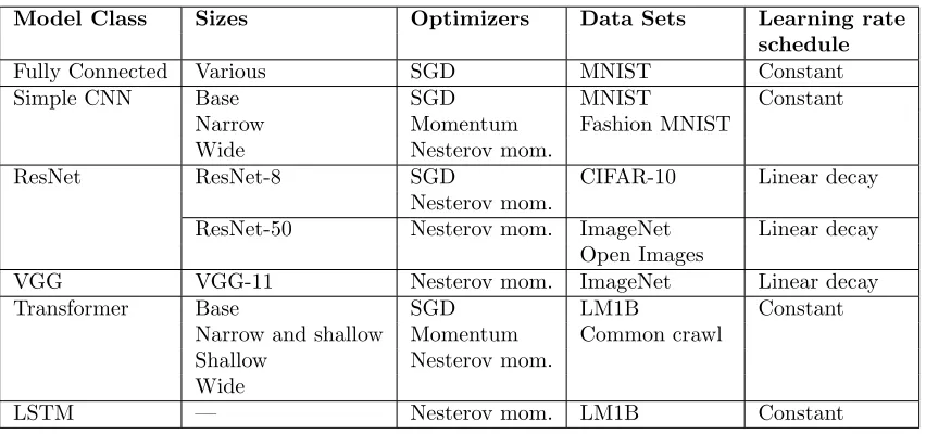
Model Class Sizes Optimizers Data Sets Learning rate

schedule

Fully Connected Various SGD MNIST Constant

Simple CNN Base SGD MNIST Constant

Narrow Momentum Fashion MNIST

Wide Nesterov mom.

ResNet ResNet-8 SGD CIFAR-10 Linear decay

Nesterov mom.

ResNet-50 Nesterov mom. ImageNet Linear decay

Open Images

VGG VGG-11 Nesterov mom. ImageNet Linear decay

Transformer Base SGD LM1B Constant

Narrow and shallow Momentum Common crawl

Shallow Nesterov mom.

Wide

LSTM — Nesterov mom. LM1B Constant

Table 2: Summary of models. See Appendix B for full details.

Measuring steps to result requires a particular value of out-of-sample error to be chosen as the goal. Ideally, we would select the best achievable error for each task and model, but since validation error is noisy, the best error is sometimes obtained unreliably. Moreover, for some workloads, the validation error continues to improve steadily beyond the maximum practical training time. Therefore, we generally tried to select the best validation error that we could achieve reliably within a practical training time.

(15)

training time for those models. We selected our decay function by running an extensive set of experiments with ResNet-50 on ImageNet (see Appendix C for details). We chose linear decay because it performed at least as well as all other schedules we tried, while also being the simplest and requiring only two additional metaparameters. In experiments that used linear decay, we specified metaparameters (η0, α, T) such that the learning rate decayed linearly fromη0 toηT =αη0. That is, the learning rate at steptis given by

ηt=

(

η0−(1−α)η0_Tt ift≤T,

αη0 ift > T.

Steps to result depends on the training metaparameters, and, for a given task and model, each batch size might have a different metaparameter configuration that minimizes steps to result. In all experiments, we independently tuned the metaparameters at each batch size, including the initial learning rateη0 and, when learning rate decay was used, the decay schedule (α, T). Also, unless otherwise specified, we used the Nesterov momentum optimizer (Sutskever et al., 2013) and tuned the momentum γ.12 Tuning anew for each batch size is extremely important since otherwise we would not be measuring steps to result as a function of batch size, rather we would be measuring steps to result as a function of batch size and the specific values of the learning rate and other metaparameters. We used quasi-random search (Bousquet et al., 2017) to tune the metaparameters with equal budgets of non-divergent13trials for different batch sizes. We selected metaparameter search spaces by hand based on preliminary experiments. The exact number of non-divergent trials needed to produce stable results depends on the search space, but 100 trials seemed to suffice in our experiments.14 If the optimal trial occurred near the boundary of the search space, or if the goal validation error was not achieved within the search space, we repeated the search with a new search space. We measured steps to result for each batch size by selecting the metaparameter trial that reached the goal validation error in the fewest number of steps.

4.1. Steps to Result Depends on Batch Size in a Similar Way Across Problems

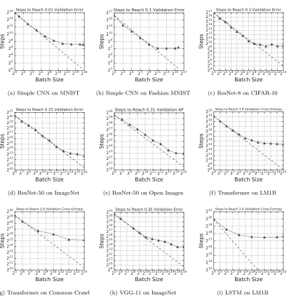
To get a sense of the basic empirical relationship, we measured the number of steps required to reach a goal validation error as a function of batch size across several different data sets and models (Figure 1). In all cases, as the batch size grows, there is an initial period of

perfect scaling(b-fold benefit, indicated with a dashed line on the plots) where the steps

needed to achieve the error goal halves for each doubling of the batch size. However, for all problems, this is followed by a region of diminishing returnsthat eventually leads to a regime of maximal data parallelismwhere additional parallelism provides no benefit whatsoever. In other words, for any given problem and without making strong assumptions about learning rates or other optimizer parameters, we can achieve both extremes suggested by theory (see Section 3.1.1). A priori, it is not obvious that every workload in our ex-periments should exhibit perfect scaling at the smallest batch sizes instead of immediately showing diminishing returns.

12. For LSTM for LM1B, we used a fixed value ofγ= 0.99. We chose this value based on initial experiments and validated that tuningγdid not significantly affect the results for batch sizes 256, 1,024, or 4,096. 13. We discarded trials with a divergent training loss, which occurred when the learning rate was too high. 14. We used 100 non-divergent trials for all experiments except Transformer Shallow on LM1B with SGD,

(16)

20 ₂2 ₂4 ₂6 ₂8 ₂10₂12₂14₂16

Batch Size

20 22 24 26 28 210 212 214 216

Steps

Steps to Reach 0.01 Validation Error

(a) Simple CNN on MNIST

21 ₂3 ₂5 ₂7 ₂9 ₂11₂13₂15₂17

Batch Size

21 23 25 27 29 211 213 215 217

Steps

(b) Simple CNN on Fashion MNIST

21₂2₂3₂4₂5₂6₂7₂8₂9₂10₂11₂12₂13

Batch Size

24 25 26 27 28 29 210 211 212 213 214 215 216 217

Steps

(c) ResNet-8 on CIFAR-10

26₂7₂8₂9₂10₂11₂12₂13₂14₂15₂16

Batch Size

210 211 212 213 214 215 216 217 218 219 220 221

Steps

(d) ResNet-50 on ImageNet

26 ₂7 ₂8 ₂9₂10₂11₂12₂13₂14₂15

Batch Size

210 211 212 213 214 215 216 217 218 219 220

Steps

Steps to Reach 0.31 Validation AP

(e) ResNet-50 on Open Images

24₂5₂6₂7₂8₂9₂10₂11₂12₂13₂14₂15

Batch Size

28 29 210 211 212 213 214 215 216 217 218 219 220

Steps

Steps to Reach 3.9 Validation Cross Entropy

(f) Transformer on LM1B

25 ₂6 ₂7 ₂8 ₂9₂10₂11₂12₂13₂14

Batch Size

210 211 212 213 214 215 216 217 218 219 220

Steps

(g) Transformer on Common Crawl

25₂6₂7₂8₂9₂10₂11₂12₂13₂14₂15₂16

Batch Size

29 210 211 212 213 214 215 216 217 218 219 220 221

Steps

(h) VGG-11 on ImageNet

24₂5₂6₂7₂8₂9₂10₂11₂12₂13₂14₂15

Batch Size

213 214 215 216 217 218 219 220 221

Steps

(i) LSTM on LM1B

Figure 1: The relationship between steps to result and batch size has the same

charac-teristic form for all problems. In all cases, as the batch size grows, there is an initial period of perfect scaling(indicated with a dashed line) where the steps needed to achieve the error goal

halves for each doubling of the batch size. Then there is a region of diminishing returns that

eventually leads to a region of maximal data parallelism where additional parallelism provides

(17)

20 ₂2 ₂4 ₂6 ₂8 ₂10 ₂12 ₂14 ₂16 Batch Size

26

27

28

29

210

211

212

213

214

215

216

217

Steps

goal error = 0.008 goal error = 0.01 goal error = 0.012 goal error = 0.014 goal error = 0.016

24 ₂5 ₂6 ₂7 ₂8 ₂9 ₂10₂11₂12₂13₂14₂15

Batch Size

212

213

214

215

216

217

218

219

220

Steps

goal error = 3.8 goal error = 3.85 goal error = 3.9 goal error = 3.95 goal error = 4.0 goal error = 4.05

(b) Transformer on LM1B

26 ₂7 ₂8 ₂9 ₂10₂11₂12₂13₂14₂15₂16

Batch Size

212

213

214

215

216

217

218

219

220

221

Steps

goal error = 0.25 goal error = 0.27 goal error = 0.29 goal error = 0.31

(c) ResNet-50 on ImageNet

Figure 2: Steps-to-result plots have a similar form for different (nearby) performance

goals. The transition points between the three regions (perfect scaling, diminishing returns, and maximal data parallelism) are nearly the same.

4.2. Validating Our Measurement Protocol

If the curves in Figure 1 were very sensitive to the goal validation error, then measuring the steps needed to reach our particular choice of the goal would not be a meaningful proxy for training speed. For small changes in the goal validation error, we do not care about vertical shifts as long as the transition points between the three scaling regions remain relatively unchanged. Figure 2 shows that varying the error goal only vertically shifts the steps-to-result curve, at least for modest variations centered around a good absolute validation error. Furthermore, although we ultimately care about out-of-sample error, if our plots looked very different when measuring the steps needed to reach a particulartraining error, then we would need to include both curves when presenting our results. However, switching to training error does not change the plots much at all (see Figure 12 in the Appendix).

Our experiments depend on extensive metaparameter tuning for the learning rate, mo-mentum, and, where applicable, the learning rate schedule. For each experiment, we verified our metaparameter search space by checking that the optimal trial was not too close to a boundary of the space. See Figures 13 and 14 in the Appendix for examples of how we verified our search spaces.

4.3. Some Models Can Exploit Much Larger Batch Sizes Than Others

(18)

20 ₂2 ₂4 ₂6 ₂8 ₂10 ₂12 ₂14 ₂16

Batch Size

2-11

22-10

-9 2-8 2-7 2-6 2-5 2-4 2-3 2-2

22-1

0

21

Steps / (Steps at B=1)

FC-1024-1024-1024 Simple CNN

(a) Fully Connected vs Simple CNN on MNIST

25 ₂6 ₂7 ₂8 ₂9 ₂10₂11₂12₂13₂14₂15₂16

Batch Size 2-9 2-8 2-7 2-6 2-5 2-4 2-3 2-2

22-1

0

21

ResNet-50 VGG-11

(b) ResNet-50 vs VGG-11 on ImageNet

24 ₂5 ₂6 ₂7 ₂8 ₂9 ₂10₂11₂12₂13₂14₂15

Batch Size 2-8 2-7 2-6 2-5 2-4 2-3 2-2

22-1

0

21

Transformer LSTM

(c) Transformer vs LSTM on LM1B

20 ₂2 ₂4 ₂6 ₂8 ₂10 ₂12 ₂14 ₂16

Batch Size

2-11

22-10

-9 2-8 2-7 2-6 2-5 2-4 2-3 2-2

22-1

0

21

FC-1024 FC-128-128-128 FC-256-256-256 FC-512-512-512 FC-1024-1024-1024 FC-2048-2048-2048

(d) Fully Connected sizes on MNIST

20 ₂2 ₂4 ₂6 ₂8 ₂10 ₂12 ₂14 ₂16

Batch Size

2-11

22-10

-9 2-8 2-7 2-6 2-5 2-4 2-3 2-2

22-1

0

21

Simple CNN Simple CNN Narrow Simple CNN Wide

(e) Simple CNN sizes on MNIST

24 ₂5 ₂6 ₂7 ₂8 ₂9 ₂10₂11 ₂12₂13₂14₂15

Batch Size 2-9 2-8 2-7 2-6 2-5 2-4 2-3 2-2

22-1

0

21

Wide Base Shallow Narrow and Shallow

(f) Transformer sizes on LM1B

Figure 3: Some models can exploit much larger batch sizes than others. Figures 3a-3c show

that some model architectures can exploit much larger batch sizes than others on the same data set. Figures 3d-3f show that varying the depth and width can affect a model’s ability to exploit larger batches, but not necessarily in a consistent way across different model architectures. All MNIST models in this Figure used plain mini-batch SGD, while all other models used Nesterov momentum. The goal validation error for each plot was chosen to allow all model variants to achieve that error.

(19)

Figures 3a–3c show that the model architecture significantly affects the relationship between batch size and the number of steps needed to reach a goal validation error. In Figure 3a, the curve for the Fully Connected model flattens later than for the Simple CNN model on MNIST (although in this case the Simple CNN model can ultimately achieve better performance than the Fully Connected model). In Figure 3b, the curve for ResNet-50 flattens much later than the curve for VGG-11, indicating that ResNet-ResNet-50 can make better use of large batch sizes on this data set. Unlike ResNet-50, VGG-11 does not use batch normalization or residual connections. Figure 3c shows that Transformer can make better use of large batch sizes than LSTM on LM1B.

Figures 3d–3f show that varying the depth and width can affect a model’s ability to exploit larger batches, but not necessarily in a consistent way across different model archi-tectures. In Figure 3d, the regions of perfect scaling, diminishing returns, and maximum useful batch size do not change much when the width is varied for the Fully Connected model on MNIST, although the shallower model seems less able to exploit larger batches than the deeper models. This contrasts with the findings of Chen et al. (2018), although they changed width and depth simultaneously while keeping the number of parameters fixed. For Simple CNN on MNIST, the relationship between batch size and steps to a goal validation error seems not to depend on width at all (Figure 15e in the Appendix shows that the curves are the same even when they-axis is not normalized). However, in Figure 3f, the curves fornarrower Transformer models on LM1B flatten later than for wider Transformer models, while the depth seems to have less of an effect. Thus, reducing width appears to allow Transformer to make more use of larger batch sizes on LM1B.

4.4. Momentum Extends Perfect Scaling to Larger Batch Sizes, but Matches Plain SGD at Small Batch Sizes

We investigated whether some optimizers can make better use of larger batches than others by experimenting with plain SGD, SGD with momentum, and Nesterov momentum on the same model and data set. Since plain SGD is a special case of both Nesterov momentum and SGD with momentum (withγ = 0 in each case), and since we tuneγ in all experiments, we expect that experiments with either of these optimizers should do no worse than plain SGD at any batch size. However, it is not clear a priori whether momentum optimizers should outperform SGD, either by taking fewer training steps or by extending the perfect scaling region to larger batch sizes.

(20)

20 ₂2 ₂4 ₂6 ₂8 ₂10₂12₂14₂16

Batch Size

24 25 26 27 28 29 210 211 212 213 214 215 216 217

Steps

SGD Momentum Nesterov Momentum

24₂5₂6₂7₂8₂9₂10₂11₂12₂13₂14₂15

Batch Size

212 213 214 215 216 217 218 219 220 221 222

Steps

Steps to Reach 3.9 Validation Cross Entropy SGD

Momentum Nesterov Momentum

(b) Transformer Shallow on LM1B

21₂2₂3₂4₂5₂6₂7₂8₂9₂10₂11₂12₂13

Batch Size

27 28 29 210 211 212 213 214 215 216 217 218

Steps

SGD

Nesterov Momentum

Figure 4: Momentum extends perfect scaling to larger batch sizes, but matches plain

SGD at small batch sizes. Nesterov momentum and SGD with momentum can both significantly reduce the absolute number of training steps to reach a goal validation error, and also significantly extend the perfect scaling region and thus better exploit larger batches than plain mini-batch SGD.

20 ₂2 ₂4 ₂6 ₂8 ₂10 ₂12 ₂14 ₂16

Batch Size 2-15 2-13 2-11 2-9 2-7 2-5 2-3 2-1 21

MNIST, 0.01 Fashion MNIST, 0.1

(a) Simple CNN on different data sets

26 ₂7 ₂8 ₂9 ₂10 ₂11₂12₂13₂14₂15 ₂16

Batch Size 2-9 2-8 2-7 2-6 2-5 2-4 2-3 2-2

22-1

0

21

ImageNet, 0.25 Open Images, 0.31

(b) ResNet-50 on different data sets

24 ₂5 ₂6 ₂7 ₂8 ₂9 ₂10₂11₂12₂13₂14₂15

Batch Size 2-8 2-7 2-6 2-5 2-4 2-3 2-2

22-1

0

21

Common Crawl, 3.9 LM1B, 3.9

(c) Transformer on different data sets

Figure 5: The data set can influence the maximum useful batch size. For the data sets

shown in this plot, these differences are not simply as straightforward as larger data sets making larger batch sizes more valuable. Appendix A.2 describes the evaluation metric used for each data set, and the plot legends show the goal metric value for each task. Figure 16 in the Appendix

contains these plots without they-axis normalized.

4.5. The Data Set Matters, at Least Somewhat

We investigated whether properties of the data set make some problems able to exploit larger batch sizes than others by experimenting with different data sets while keeping the model and optimizer fixed. We approached this in two ways: (i) by testing the same model on completely different data sets, and (ii) by testing the same model on different subsets of the same data set. We normalized they-axis of all plots in this section in the same way as Section 4.3. Appendix D contains all plots in this section without the y-axis normalized.

(21)

20 ₂2 ₂4 ₂6 ₂8 ₂10 ₂12 ₂14 ₂16 Batch Size

22-10

-9

2-8

2-7

2-6

2-5

2-4

2-3

2-2

22-1

0

21

100% of Images, 0.02 50% of Images, 0.02 25% of Images, 0.02 12.5% of Images, 0.02

(a) Simple CNN on MNIST subsets

26 ₂7 ₂8 ₂9 ₂10 ₂11 ₂12 ₂13 ₂14 ₂15 ₂16

Batch Size

2-9

2-8

2-7

2-6

2-5

2-4

2-3

2-2

22-1

0

21

100% of Images, 0.25 50% of Images, 0.3 50% of Classes, 0.3

(b) ResNet-50 on ImageNet subsets

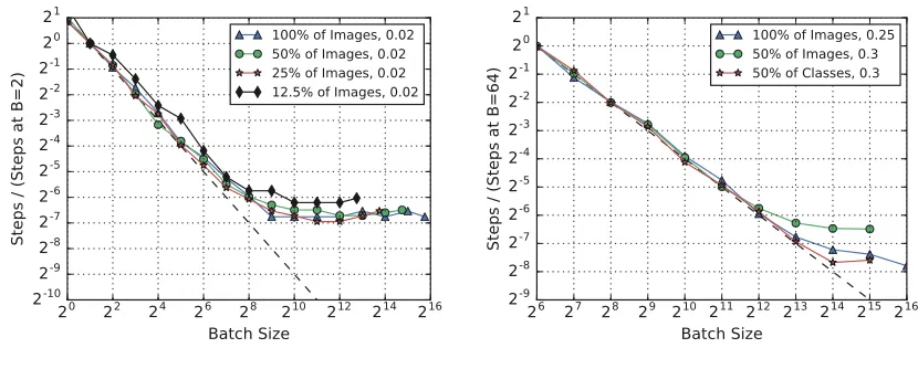
Figure 6: Investigating the effect of data set size. At least for MNIST, any effect of subset

size on the maximum useful batch size is extremely small or nonexistent. For ImageNet, the random subset of half the images deviates from perfect scaling sooner than the full data set, but the curve for the subset with half the classes is very close to the curve for the full data set and, if anything, deviates from perfect scaling later. Appendix A.2 describes the evaluation metric used for each data set, and the plot legends show the goal metric value for each task. Figure 17 in the Appendix

contains these plots without they-axis normalized.

Fashion MNIST is the same size as MNIST, Open Images is larger than ImageNet, and Common Crawl is far larger than LM1B, these differences are not simply as straightforward as larger data sets making larger batch sizes more valuable.

To disentangle the effects from changes to the distribution and changes to the number of examples, we generated steps to result vs batch size plots for different random subsets of MNIST (Figure 6a) and ImageNet (Figure 6b). For MNIST, we selected subsets of different sizes, while for ImageNet, we selected a random subset of half the images and a similar sized subset that only includes images from half of the classes. At least on MNIST, any effect on the maximum useful batch size is extremely small or nonexistent. For ImageNet, Figure 6b shows that the random subset of half the images deviates from perfect scaling sooner than the full data set, but the curve for the subset with half the classes is very close to the curve for the full data set and, if anything, deviates from perfect scaling later, even though it contains roughly the same number of images as the random subset.

4.6. Regularization Can Be More Helpful at Some Batch Sizes Than Others

(22)

26 ₂7 ₂8 ₂9 ₂10 ₂11 ₂12 ₂13 ₂14 ₂15 ₂16 Batch Size

0.235 0.240 0.245 0.250 0.255 0.260 0.265

Validation Error

Best Validation Error Per Batch Size

Label Smoothing = 0.00 Label Smoothing = 0.01 Label Smoothing = 0.10

(a) Label smoothing benefits larger batch sizes, but has no apparent effect for smaller batch sizes.

26 ₂7 ₂8 ₂9 ₂10 ₂11 ₂12 ₂13 ₂14 ₂15 ₂16

Batch Size

210

211

212

213

214

215

216

217

218

219

220

221

Steps

Steps to Reach 0.25 Validation Error

Label Smoothing = 0.00 Label Smoothing = 0.01 Label Smoothing = 0.10

(b) Label smoothing has no apparent effect on training speed, provided the goal error is achieved.

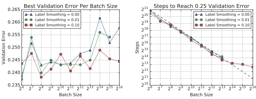
Figure 7: Regularization can be more helpful at some batch sizes than others. Plots are

for ResNet-50 on ImageNet. Each point corresponds to a different metaparameter tuning trial, so the learning rate, Nesterov momentum, and learning rate schedule are independently chosen for each point. The training budget is fixed for each batch size, but varies between batch sizes.

We confirmed that label smoothing reduced overfitting at large batch sizes for ResNet-50 on ImageNet (see Figure 18 in the Appendix). This is consistent with the idea that noise from small batch training is a form of implicit regularization (e.g. Goodfellow et al., 2016). However, although our results show that other forms of regularization can serve in place of this noise, it might be difficult to select and tune other forms of regularization for large batch sizes. For example, we unsuccessfully tried to control overfitting with larger batch sizes by increasing theL2 weight penalty and by applying additive Gaussian gradient noise before we obtained good results with label smoothing.

Finally, we also tried label smoothing with Simple CNN on MNIST and Fashion MNIST, and found that it generally helpedallbatch sizes, with no consistent trend of helping smaller or larger batch sizes more (see Figure 19 in the Appendix), perhaps because these data sets are sufficiently small and simple that overfitting is an issue at all batch sizes.

4.7. The Best Learning Rate and Momentum Vary with Batch Size

(23)

20 ₂2 ₂4 ₂6 ₂8 ₂10₂12 ₂14₂16

Batch Size

2-8 2-6 2-4 22-2 0 22 24 26 28

Learning Rate / (1 - Momentum)

Optimal Effective Learning Rate Linear Heuristic Square Root Heuristic

21 ₂3 ₂5 ₂7 ₂9 ₂11₂13 ₂15₂17

Batch Size

2-5 2-3 22-1 1 23 25 27 29 211 213

(b) Simple CNN on Fashion MNIST

21₂2₂3₂4₂5₂6₂7₂8₂9₂10₂11₂12₂13

Batch Size

2-7 2-6 2-5 2-4 2-3 2-2 22-10 21 22 23 24 25 26

26 ₂7₂8 ₂9₂10₂11₂12₂13₂14₂15₂16

Batch Size

2-3 2-2 22-1 0 21 22 23 24 25 26 27 28

(d) ResNet-50 on ImageNet

26 ₂7 ₂8 ₂9₂10₂11₂12₂13₂14₂15

Batch Size

2-5 2-4 2-3 2-2 22-10 21 22 23 24 25 26 27

(e) ResNet-50 on Open Images

24₂5₂6₂7₂8₂9₂10₂11₂12₂13₂14₂15

Batch Size

2-6 2-5 2-4 2-3 2-2 22-10 21 22 23 24 25 26

(f) Transformer on LM1B

25 ₂6 ₂7 ₂8 ₂9 ₂10₂11₂12₂13₂14

Batch Size

2-5 2-4 2-3 2-2 22-1 0 21 22 23 24 25

(g) Transformer on Common Crawl

25₂6₂7₂8₂9₂10₂11₂12₂13₂14₂15₂16

Batch Size

2-6 2-5 2-4 2-3 2-2 22-10 21 22 23 24 25 26

(h) VGG-11 on ImageNet

24₂5₂6₂7₂8₂9₂10₂11₂12₂13₂14₂15

Batch Size

2-8 2-7 2-6 2-5 2-4 2-3 2-2 22-10 21 22 23 24

(i) LSTM on LM1B

Figure 8: Optimal effective learning rates do not always follow linear or square root

(24)

10-4 ₁₀-3 ₁₀-2 ₁₀-1 10-6 10-5 10-4 10-3 10-2 10-1 100 101 1-Momentum

Batch Size 128

Goal Achieved Goal Not Achieved Infeasible

10-4 ₁₀-3 ₁₀-2 ₁₀-1

10-6 10-5 10-4 10-3 10-2 10-1 100

101 Batch Size 256

10-4 ₁₀-3 ₁₀-2 ₁₀-1

10-6 10-5 10-4 10-3 10-2 10-1 100

101 Batch Size 512

10-4 ₁₀-3 ₁₀-2 ₁₀-1

Learning Rate 10-6 10-5 10-4 10-3 10-2 10-1 100 101 1-Momentum

Batch Size 1024

10-4 ₁₀-3 ₁₀-2 ₁₀-1

Learning Rate 10-6 10-5 10-4 10-3 10-2 10-1 100

101 Batch Size 2048

10-4 ₁₀-3 ₁₀-2 ₁₀-1

Learning Rate 10-6 10-5 10-4 10-3 10-2 10-1 100

101 Batch Size 4096

Goal Not Achieved Infeasible

(a)Transformer on LM1B with a training budget of one epoch.

10-4 ₁₀-3 ₁₀-2 ₁₀-1

10-6 10-5 10-4 10-3 10-2 10-1 100 101 1-Momentum

Batch Size 512

10-4 ₁₀-3 ₁₀-2 ₁₀-1

10-6 10-5 10-4 10-3 10-2 10-1 100

101 Batch Size 1024

10-4 ₁₀-3 ₁₀-2 ₁₀-1

10-6 10-5 10-4 10-3 10-2 10-1 100

101 Batch Size 2048

10-4 ₁₀-3 ₁₀-2 ₁₀-1

Learning Rate 10-6 10-5 10-4 10-3 10-2 10-1 100 101 1-Momentum

Batch Size 4096

10-4 ₁₀-3 ₁₀-2 ₁₀-1

Learning Rate 10-6 10-5 10-4 10-3 10-2 10-1 100

101 Batch Size 8192

10-4 ₁₀-3 ₁₀-2 ₁₀-1

Learning Rate 10-6 10-5 10-4 10-3 10-2 10-1 100

101 Batch Size 16384

(b)Transformer on LM1B with a training budget of 25,000 steps.

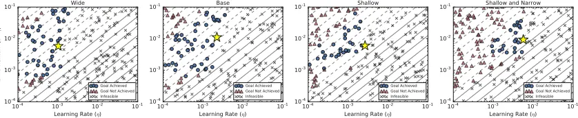
Figure 9: With increasing batch size, the region in metaparameter space corresponding

to rapid training in terms of epochs becomes smaller, while the region in metaparameter space corresponding to rapid training in terms of step-count grows larger. Yellow stars are the trials that achieved the goal in the fewest number of steps. Contours indicate the effective

learning rateηeff₌ η

(25)

10-4 ₁₀-3 ₁₀-2 ₁₀-1

Learning Rate (η)

10-4

10-3

10-2

10-1

1-Mo

m

en

tu

m

(

1

−

γ

)

Wide

10-4 ₁₀-3 ₁₀-2 ₁₀-1

Learning Rate (η)

10-4

10-3

10-2

10-1 Base

10-4 ₁₀-3 ₁₀-2 ₁₀-1

Learning Rate (η)

10-4

10-3

10-2

10-1 Shallow

10-4 ₁₀-3 ₁₀-2 ₁₀-1

Learning Rate (η)

10-4

10-3

10-2

10-1 Shallow and Narrow

Figure 10: Smaller models have larger stable learning rates for Transformer on LM1B.

Plots are for different sizes of Transformer on LM1B with a batch size of 1024, a goal validation cross entropy error of 4.2, and a training budget of 50,000 steps. Contours indicate the effective

learning rateηeff₌ η

1−γ. Infeasible trials are those that resulted in divergent training.

We further investigated the relationship between learning rate, momentum, and training speed by examining our metaparameter search spaces for different batch sizes and model sizes. For this analysis, we used Transformer on LM1B with Nesterov momentum because the metaparameter search spaces are consistent between all batch and model sizes, and can be easily visualized because they consist only of the constant learning rate η and the momentum γ. We observe the following behaviors:

• With increasing batch size, the region in metaparameter space corresponding to rapid training in terms of epochs becomes smaller (Figure 9a, consistent with the findings of Breuel, 2015b), while the region in metaparameter space corresponding to rapid training in terms of step-count grows larger (Figure 9b, although it eventually plateaus for batch sizes in the maximal data parallelism regime). Thus, with a fixed error goal and in a setting where training epochs are constrained (e.g. a compute budget), it may become more challenging to choose good values for the metaparameters with increasing batch size. Conversely, with a fixed error goal and in a setting where training steps are constrained (e.g. a wall-time budget), it may become easier to choose good values for the metaparameters with increasing batch size.

• The metaparameters yielding the fastest training are typically on the edge of the feasi-ble region of the search space (Figure 9). In other words, small changes in the optimal metaparameters might make training diverge. This behavior may pose a challenge for metaparameter optimization techniques, such as Gaussian Process approaches, that assume a smooth relationship between metaparameter values and model performance. It could motivate techniques such as learning rate warm-up that enable stability at larger eventual learning rates, since the maximum stable learning rate depends on the current model parameters. We did not observe the same behavior for ResNet-50 on ImageNet. Figure 20 in the Appendix shows the results for a range of effective learning rates near the optimum for ResNet-50 on ImageNet and Transformer on LM1B.

(26)

4.8. Solution Quality Depends on Compute Budget More Than Batch Size

We investigated the relationship between batch size and out-of-sample error for Simple CNN on MNIST and Fashion MNIST, and for two sizes of Transformer on LM1B. For each task, we ran a quasi-random metaparameter search over the constant learning rate η and Nesterov momentum γ. For MNIST and Fashion MNIST, we also added label smoothing and searched over the label smoothing parameter in {0,0.1} to mitigate any confounding effects of overfitting (see Section 4.6). We ran 100 metaparameter trials for each batch size with a large practical wall-time budget.

To disentangle the effects of the batch size from the compute budget, we compared batch sizes subject to budgets of either training steps or training epochs. For each batch size and compute budget, we found the model checkpoint that achieved the best validation accuracy across all metaparameter trials, and across all training steps that fell within the compute budget. Figure 11 shows the validation error for these best-validation-error checkpoints, as a function of batch size, for a range of compute budgets. We observe that, subject to a budget on training steps, larger batch sizes achieve better out-of-sample error than smaller batch sizes, but subject to a budget on training epochs, smaller batch sizes achieve better out-of-sample error than larger batch sizes. These observations are likely explained by the observations that, for a fixed number of training steps, larger batch sizes train on more data, while for a fixed number of epochs, smaller batch sizes perform more training steps.

The workloads in Figure 11 represent two distinct modes of neural network training. For the small MNIST and Fashion MNIST data sets, we used training budgets that would saturate (or almost saturate) performance at each batch size. In other words, out-of-sample error cannot be improved by simply increasing the budget, with caveats due to practical limitations on our ability to find optimal values for the metaparameters. Figures 11a and 11b show that differences in maximum performance between batch sizes on these data sets are very small (see Figures 23 and 24 in the Appendix for zoomed versions of these plots). We cannot rule out that any differences at this magnitude are due to noise from metaparameter choices and training stochasticity. Thus, for these workloads at least, the effect of batch size on solution quality is either very small or nonexistent. On the other hand, we cannot saturate performance with Transformer on LM1B within a practical training time. In this case, Figures 11c and 11d show that the best error is simply achieved by the largest compute budget.