Regularized Evolution for Image Classifier Architecture Search

The Thirty-Third AAAI Conference on Artificial Intelligence (AAAI-19)

Regularized Evolution for Image Classifier Architecture Search

Esteban Real,

Alok Aggarwal, Yanping Huang, Quoc V. Le

Correspondence to E. Real at [email protected]

Abstract

The effort devoted to hand-crafting neural network image classifiers has motivated the use of architecture search to dis-cover them automatically. Although evolutionary algorithms have been repeatedly applied to neural network topologies, the image classifiers thus discovered have remained inferior to human-crafted ones. Here, we evolve an image classifier—

AmoebaNet-A—that surpasses hand-designs for the first time. To do this, we modify the tournament selection evolution-ary algorithm by introducing an age property to favor the younger genotypes. Matching size, AmoebaNet-A has com-parable accuracy to current state-of-the-art ImageNet models discovered with more complex architecture-search methods. Scaled to larger size, AmoebaNet-A sets a new state-of-the-art 83.9% top-1 / 96.6% top-5 ImageNet accuracy. In a con-trolled comparison against a well known reinforcement learn-ing algorithm, we give evidence that evolution can obtain re-sults faster with the same hardware, especially at the earlier stages of the search. This is relevant when fewer compute re-sources are available. Evolution is, thus, a simple method to effectively discover high-quality architectures.

Introduction

Until recently, most state-of-the-art image classifier archi-tectures have been manually designed by human experts (Krizhevsky, Sutskever, and Hinton 2012; Szegedy et al. 2015; He et al. 2016; Huang et al. 2017; Hu, Shen, and Sun 2018). To speed up the process, researchers have looked into automated methods (Baker et al. 2017a; Zoph and Le 2016; Miikkulainen et al. 2017; Real et al. 2017; Xie and Yuille 2017; Suganuma, Shirakawa, and Nagao 2017; Liu et al. 2018a; Pham et al. 2018). These methods are now col-lectively known as architecture-search algorithms. A tra-ditional approach isneuro-evolution of topologies (Miller, Todd, and Hegde 1989; Angeline, Saunders, and Pollack 1994; Stanley and Miikkulainen 2002). Improved hardware now allows scaling up evolution to produce high-quality image classifiers (Real et al. 2017; Xie and Yuille 2017; Liu et al. 2018b). Yet, the architectures produced by evolu-tionary algorithms / genetic programming have not reached the accuracy of those directly designed by human experts. Here we evolve image classifiers that surpass hand-designs.

∗

E. Real, A. Aggarwal, and Y. Huang contributed equally. Copyright c2019, Association for the Advancement of Artificial Intelligence (www.aaai.org). All rights reserved.

To do this, we make two additions to the standard evo-lutionary process. First, we propose a change to the well-established tournament selection evolutionary algorithm (Goldberg and Deb 1991) that we refer to as aging evo-lution orregularizedevolution. Whereas in tournament se-lection, the best genotypes (architectures) are kept, we pro-pose to associate each genotype with an age, and bias the tournament selection to choose the younger genotypes. We will show that this change turns out to make a difference. The connection to regularization will be clarified in the Dis-cussion section. Second, we implement the simplest set of mutations that would allow evolving in the NASNet search space (Zoph et al. 2018). This search space associates con-volutional neural network architectures with small directed graphs in which vertices represent hidden states and labeled edges represent common network operations (such as con-volutions or pooling layers). Our mutation rules only alter architectures by randomly reconnecting the origin of edges to different vertices and by randomly relabeling the edges, covering the full search space.

Searching in the NASNet space allows a controlled com-parison between evolution and the original method for which the space was designed, reinforcement learning (RL). Thus, this paper presents the first comparative case study of architecture-search algorithms for the image classifica-tion task. Within this case study, we will demonstrate that evolution can attain similar results with a simpler method, as will be shown in the Discussion section. In particular, we will highlight that in all our experiments evolution searched faster than RL and random search, especially at the earlier stages, which is important when experiments cannot be run for long times due to compute resource limitations.

Despite its simplicity, our approach works well in our benchmark against RL. It also evolved a high-quality model, which we name AmoebaNet-A. This model is competitive with the best image classifiers obtained by any other algo-rithm today at similar sizes (82.8% top-1 / 96.1% top-5 Im-ageNet accuracy). When scaled up, it sets a new state-of-the-art accuracy (83.9% top-1 / 96.6% top-5 ImageNet ac-curacy).

Related Work

(Elsken, Metzen, and Hutter 2018) literature on image clas-sifier architecture search, including successful RL studies (Zoph and Le 2016; Baker et al. 2017a; Zoph et al. 2018; Liu et al. 2018a; Zhong, Yan, and Liu 2018; Cai et al. 2018) and evolutionary studies like those mentioned in the Intro-duction. Other methods have also been applied: cascade-correlation (Fahlman and Lebiere 1990), boosting (Cortes et al. 2017), hill-climbing (Elsken, Metzen, and Hutter 2017), MCTS (Negrinho and Gordon 2017), SMBO (Mendoza et al. 2016; Liu et al. 2018a), and random search (Bergstra and Bengio 2012), and grid search (Zagoruyko and Komodakis 2016). Some methods even forewent the idea of independent architectures (Saxena and Verbeek 2016). There is much architecture-search work beyond image classification too, but that is outside our scope.

Even though some methods stand out due to their effi-ciency (Suganuma, Shirakawa, and Nagao 2017; Pham et al. 2018), many approaches use large amounts of resources. Several recent papers reduced the compute cost through progressive-complexity search stages (Liu et al. 2018a), hy-pernets (Brock et al. 2018), accuracy prediction (Baker et al. 2017b; Klein et al. 2017; Domhan, Springenberg, and Hutter 2017), warm-starting and ensembling (Feurer et al. 2015), parallelization, reward shaping and early stopping (Zhong, Yan, and Liu 2018) or Net2Net transformations (Cai et al. 2018). Most of these methods could in principle be applied to evolution too, but this is beyond the scope of this paper.

A popular approach to evolution has been through gen-erationalalgorithms,e.g. NEAT (Stanley and Miikkulainen 2002). In these, all models in the population must finish training before the next generation is computed. Genera-tional evolution becomes inefficient in a distributed environ-ment where a different machine is used to train each model: machines that train faster models finish earlier and must wait idle until all machines are ready. Real-time algorithms ad-dress this issue,e.g. rtNEAT (Stanley, Bryant, and Miikku-lainen 2005) and tournament selection (Goldberg and Deb 1991). Unlike the generational algorithms, however, these discard models according to their performance or do not dis-card them at all, resulting in models that remain alive in the population for a long time—even for the whole experiment. We will present evidence that the finite lifetimes of aging evolution can give better results than direct tournament se-lection, while retaining its efficiency.

An existing paper (Hornby 2006) uses a concept ofage

but in a very different way than we do. In that paper, age is assigned to genes to divide a constant-size population into groups calledage-layers. Each layer contains individ-uals with genes of similar ages. Only after the genes have survived a certain age-gap, they can make it to the next layer. The goal is to restrict competition (the newly intro-duced genes cannot be immediately out-competed by highly selected older ones). Their algorithm requires the introduc-tion of two addiintroduc-tional meta-parameters (size of the age-gap and number of age-layers). In contrast, in our algorithm, an

ageis assigned to the individuals (not the genes) and is only used to track which is the oldest individual in the popula-tion. This permits removing such oldest individual at each cycle (keeping a constant population size). Our approach,

therefore, is in line with our goal of keeping the method as simple as possible. In particular, our method remains simi-lar to nature (where the young are less likely to die than the very old) and it requires no additional meta-parameters.

Methods

This section contains a readable description of the methods. The Methods Details section gives additional information.

Search Space

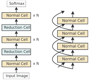
All experiments use the NASNet search space(Zoph et al. 2018). This is a space of image classifiers, all of which have the fixed outer structure indicated in Figure 1 (left): a feed-forward stack of Inception-like modules called cells. Each cell receives a direct input from the previous cell (as de-picted) and a skip input from the cell before it (Figure 1, right). The cells in the stack are of two types: the normal celland thereduction cell. All normal cells are constrained to have the same architecture, as are reduction cells, but the architecture of the normal cells is independent of that of the reduction cells. Other than this, the only difference between them is that every application of the reduction cell is fol-lowed by a stride of 2 that reduces the image size, whereas normal cells preserve the image size. As can be seen in the figure, normal cells are arranged in three stacks of N cells. The goal of the architecture-search process is to discover the architectures of the normal and reduction cells.

Figure 1: NASNet Search Space outer structure (Zoph et al. 2018). LEFT: the full outer structure, omitting skip inputs for clarity. RIGHT: detailed view with the skip inputs.

As depicted in Figure 1 (right) and Figure 2, each cell has two input activation tensors and one output. The very first cell takes two copies of the input image. After that, the inputs are the outputs of the previous two cells.

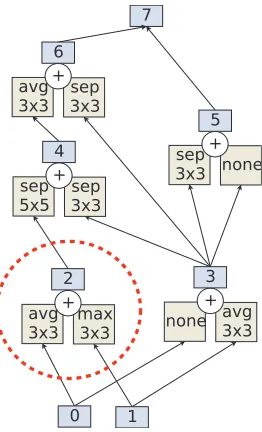
Figure 2: NASNet Search Space cell structure (Zoph et al. 2018). Example of a cell. Dotted line demarcates a pairwise combination.

hidden state, applying another op to another existing hidden state, and adding the results to produce a new hidden state. Ops belong to a fixed set of common convnet operations such as convolutions and pooling layers. Repeating hidden states or operations within a combination is permitted. In the cell example of Figure 2, the first pairwise combination ap-plies a 3x3 average pool op to hidden state 0 and a 3x3 max pool op to hidden state 1, in order to produce hidden state 2. The next pairwise combination can now choose from hidden states 0, 1, and 2 to produce hidden state 3 (chose 0 and 1 in Figure 2), and so on. After exactly five pairwise combina-tions, any hidden states that remain unused (hidden states 5 and 6 in Figure 2) are concatenated to form the output of the cell (hidden state 7).

A given architecture is fully specified by the five pairwise combinations that make up the normal cell and the five that make up the reduction cell. Once the architecture is speci-fied, the model still has two free parameters that can be used to alter its size (and its accuracy): the number of normal cells per stack (N) and the number of output filters of the convo-lution ops (F). N and F are determined manually.

Evolutionary Algorithm

The evolutionary method we used is summarized in Algo-rithm 1. It keeps a population of P trained models through-out the experiment. The population is initialized with models with random architectures (“while|population|” in Algo-rithm 1). All architectures that conform to the search space described are possible and equally likely.

After this, evolution improves the initial population in cy-cles (“while|history|” in Algorithm 1). At each cycle, it samples S random models from the population, each drawn uniformly at random with replacement. The model with the highest validation fitness within this sample is selected as the

Algorithm 1Aging Evolution (i.e. Regularized Evolution)

population←empty queue .The population.

history←∅ .Will contain all models.

while|population|< P do .Initialize population.

model.arch←RANDOMARCHITECTURE() model.accuracy←TRAINANDEVAL(model.arch)

addmodelto right ofpopulation

addmodelto history

end while

while|history|< Cdo .Evolve forCcycles.

sample←_∅ .Parent candidates.

while|sample|< Sdo

candidate←random element frompopulation .The element stays in thepopulation. addcandidatetosample

end while

parent←highest-accuracy model insample child.arch←MUTATE(parent.arch)

child.accuracy←TRAINANDEVAL(child.arch)

addchildto right ofpopulation

addchildtohistory

removedeadfrom left ofpopulation .Oldest. discarddead

end while

returnhighest-accuracy model inhistory

parent. A new architecture, called thechild, is constructed from the parent by the application of a transformation called amutation. A mutation causes a simple and random modi-fication of the architecture and is described in detail below. Once the child architecture is constructed, it is then trained, evaluated, and added to the population. This process is called tournament selection (Goldberg and Deb 1991).

It is common in tournament selection to keep the popu-lation size fixed at the initial value P. This is often accom-plished with an additional step within each cycle: discarding (orkilling) the worst model in the random S-sample. We will refer to this approach as non-aging evolution. In contrast, in this paper we prefer a novel approach: killing the oldest model in the population—that is, removing from the popu-lation the model that was trained the earliest (“removedead

from left of pop” in Algorithm 1). This favors the newer models in the population. We will refer to this approach as

aging evolution. In the context of architecture search, aging evolution allows us to explore the search space more, instead of zooming in on good models too early, as non-aging evo-lution would (see Discussion section for details).

In practice, this algorithm is parallelized by distributing the “while |history|” loop in Algorithm 1 over multiple workers. Intuitively, the mutations can be thought of as pro-viding exploration, while the parent selection provides ex-ploitation. The parameter S controls the aggressiveness of the exploitation:S = 1reduces to a type of random search and2≤S≤Pleads to evolution of varying greediness.

above, we use two main mutations that we call thehidden state mutation and the op mutation. A third mutation, the identity, is also possible. Only one of these mutations is ap-plied in each cycle, choosing between them at random.

Figure 3: Illustration of the two mutation types.

The hidden state mutation consists of first making a ran-dom choice of whether to modify the normal cell or the re-duction cell. Once a cell is chosen, the mutation picks one of the five pairwise combinations uniformly at random. Once the pairwise combination is picked, one of the two elements of the pair is chosen uniformly at random. The chosen ele-ment has one hidden state. This hidden state is now replaced with another hidden state from within the cell, subject to the constraint that no loops are formed (to keep the feed-forward nature of the convnet). Figure 3 (top) shows an example.

The op mutation behaves like the hidden state mutation as far as choosing one of the two cells, one of the five pair-wise combinations, and one of the two elements of the pair. Then it differs in that it modifies the op instead of the hidden state. It does this by replacing the existing op with a random choice from a fixed list of ops (see Methods Details). Fig-ure 3 (bottom) shows an example.

Baseline Algorithms

Our main baseline is the application of RL to the same search space. RL was implemented using the algorithm and code in the baseline study (Zoph et al. 2018). An LSTM con-troller outputs the architectures, constructing the pairwise combinations one at a time, and then gets a reward for each architecture by training and evaluating it. More detail can be found in the baseline study. We also compared against ran-dom search (RS). In our RS implementation, each model is constructed randomly so that all models in the search space are equally likely, as in the initial population in the evolu-tionary algorithm. In other words, the models in RS exper-iments arenotconstructed by mutating existing models, so as to make new models independent from previous ones.

Experimental Setup

We ran controlled comparisons at scale, ensuring identical conditions for evolution, RL and random search (RS). In particular, all methods usedthe samecomputer code for net-work construction, training and evaluation. Experiments al-ways searched on the CIFAR-10 dataset (Krizhevsky and Hinton 2009).

As in the baseline study, we first performed architec-ture search over small models (i.e. small N and F) until 20k models were evaluated. After that, we used themodel augmentation trick (Zoph et al. 2018): we took architec-tures discovered by the search (e.g. the output of an evo-lutionary experiment) and turned them into a full-size, ac-curate models. To accomplish this, we enlarged the mod-els by increasing N and F so the resulting model sizes would match the baselines, and we trained the enlarged models for a longer time on the CIFAR-10 or the Ima-geNet classification datasets (Krizhevsky and Hinton 2009; Deng et al. 2009). For ImageNet, a stem was added at the input of the model to reduce the image size, as shown in Figure 6 (left). This is the same procedure as in the baseline study. To produce the largest model (see last paragraph of Results section), we increased N and F until we ran out of memory. Actual values of N and F for all models are listed in the Methods Details section.

Methods Details

This section complements the Methods section with the de-tails necessary to reproduce our experiments. Possible ops: none (identity); 3x3, 5x5 and 7x7 separable (sep.) convolu-tions (convs.); 3x3 average (avg.) pool; 3x3 max pool; 3x3 dilated (dil.) sep. conv.; 1x7 then 7x1 conv. Evolved with

P=100,S=25. CIFAR-10 dataset (Krizhevsky and Hinton 2009) with 5k withheld examples for validation. Standard ImageNet dataset (Deng et al. 2009), 1.2M 331x331 images and 1k classes; 50k examples withheld for validation; stan-dard validation set used for testing. During the search phase, each model trained for 25 epochs; N=3/F=24, 1 GPU. Each experiment ran on 450 K40 GPUs for 20k models (approx. 7 days). To optimize evolution, we tried 5 configurations with P/S of: 100/2, 100/50, 20/20, 100/25, 64/16, best was 100/25. The probability of the identity mutation was fixed at the small, arbitrary value of 0.05 and was not tuned. Other mutation probabilities were uniform, as described in the Methods. To optimize RL, started with parameters already tuned in the baseline study and further optimized learning rate in 8 configurations: 0.00003, 0.00006, 0.00012, 0.0002, 0.0004, 0.0008, 0.0016, 0.0032; best was 0.0008. To avoid selection bias, plots do not include optimization runs, as was decided a priori. Best few (20) models were selected from each experiment and augmented to N=6/F=32, as in base-line study; batch 128, SGD with momentum rate 0.9, L2 weight decay5×10−4_{, initial lr 0.024 with cosine decay, 600}

opti-mizer with 0.9 decay and=0.1,4×10−5weight decay, 0.1 label smoothing, auxiliary softmax weighted by 0.4; dropout probability 0.5; ScheduledDropPath to 0.7 probability (as in baseline—note that this trick only contributes 0.3% top-1 ImageNet acc.); 0.001 initial lr, decaying every 2 epochs by 0.97. Largest model used N=6/F=448. F always refers to the number of filters of convolutions in the first stack; after each reduction cell, this number is doubled. Wherever applicable, we used the same conditions as the baseline study.

Results

Comparison With RL and RS Baselines

Currently, reinforcement learning (RL) is the predominant method for architecture search. In fact, today’s state-of-the-art image classifiers have been obtained by architec-ture search with RL (Zoph et al. 2018; Liu et al. 2018a). Here we seek to compare our evolutionary approach against their RL algorithm. We performed large-scale side-by-side architecture-search experiments on CIFAR-10. We first op-timized the hyper-parameters of the two approaches inde-pendently (details in Methods Details section). Then we ran 5 repeats of each of the two algorithms—and also of random search (RS).

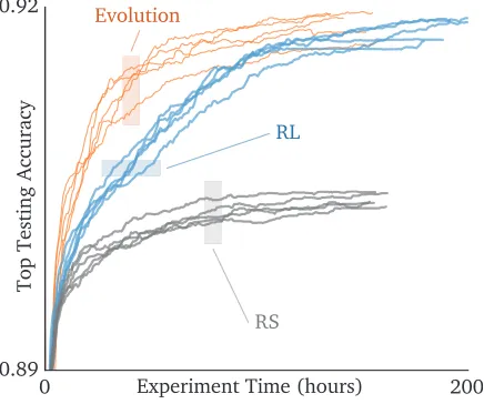
Figure 4: Time-course of 5 identical large-scale experiments for each algorithm (evolution, RL, and RS), showing ac-curacy before augmentation on CIFAR-10. All experiments were stopped when 20k models were evaluated, as done in the baseline study. Note this plot does not show the compute cost of models, which was higher for the RL ones.

Figure 4 shows the model accuracy as the experiments progress, highlighting that evolution yielded more accurate models at the earlier stages, which could become important in a resource-constrained regime where the experiments may have to be stopped early (for example, when 450 GPUs for 7 days is too much). At the later stages, if we allow to run for the full 20k models (as in the baseline study), evolution produced models with similar accuracy. Both evolution and

RL compared favorably against RS. It is important to note that the vertical axis of Figure 4 does not present the com-pute cost of the models, only their accuracy. Next, we will consider their compute cost as well.

As in the baseline study, the architecture-search experi-ments above were performed over small models, to be able to train them quicker. We then used themodel augmentation

trick (Zoph et al. 2018) by which we take an architecture discovered by the search (e.g. the output of an evolutionary experiment) and turn it into a full-size, accurate model, as described in the Methods.

Figure 5: Final augmented models from 5 identical architecture-search experiments for each algorithm, on CIFAR-10. Each marker corresponds to the top models from one experiment.

Figure 5 compares the augmented top models from the three sets of experiments. It shows test accuracy and model compute cost. The latter is measured in FLOPs, by which we mean the total count of operations in the forward pass, so lower is better. Evolved architectures had higher accuracy (and similar FLOPs) than those obtained with RS, and lower FLOPs (and similar accuracy) than those obtained with RL. Number of parameters showed similar behavior to FLOPs. Therefore, evolution occupied the ideal relative position in this graph within the scope of our case study.

Table 1: CIFAR-10 testing set results for AmoebaNet-A, compared to top model reported in the baseline study.

Model # Params Test Error (%)

NASNet-A (baseline) 3.3 M 3.41

AmoebaNet-A (N=6, F=32) 2.6 M 3.40±0.08

AmoebaNet-A (N=6, F=36) 3.2 M 3.34±0.06

Figure 6: AmoebaNet-A architecture. The overall model (Zoph et al. 2018) (LEFT) and the AmoebaNet-A normal cell (MID-DLE) and reduction cell (RIGHT).

by the baseline study. We select our evolved architecture with highest validation accuracy and call it AmoebaNet-A

(Figure 6). Table 1 compares its test accuracy with the top model of the baseline study, NASNet-A. Such a comparison is not entirely controlled, as we have no way of ensuring the network training code was identical and that the same number of experiments were done to obtain the final model. The table summarizes the results of training AmoebaNet-A at sizes comparable to a NASNet-A version, showing that AmoebaNet-A is slightly more accurate (when matching model size) or considerably smaller (when matching accu-racy). We did not train our model at larger sizes on CIFAR-10. Instead, we moved to ImageNet to do further compar-isons in the next section.

ImageNet Results

Following the accepted standard, we compare our top model’s classification accuracy on the popular ImageNet dataset against other top models from the literature. Again, we use AmoebaNet-A, the model with the highest validation accuracy on CIFAR-10 among our evolution experiments. We highlight that the model was evolved on CIFAR-10 and then transferred to ImageNet, so the evolved architecture

cannot have overfit the ImageNet dataset. When re-trained on ImageNet, AmoebaNet-A performs comparably to the baseline for the same number of parameters (Table 2, model with F=190).

Finally, we focused on AmoebaNet-A exclusively and en-larged it, setting a new state-of-the-art accuracy on Ima-geNet of 83.9%/96.6% top-1/5 accuracy with 469M param-eters (Table 2, model with F=448). Such high parameter counts may be beneficial in training other models too but we have not managed to do this yet.

Discussion

This section will suggest directions for future work, which we will motivate by speculating about the evolutionary pro-cess and by summarizing additional minor results. The de-tails of these minor results have been relegated to the supple-ments, as they are not necessary to understand or reproduce our main results above.

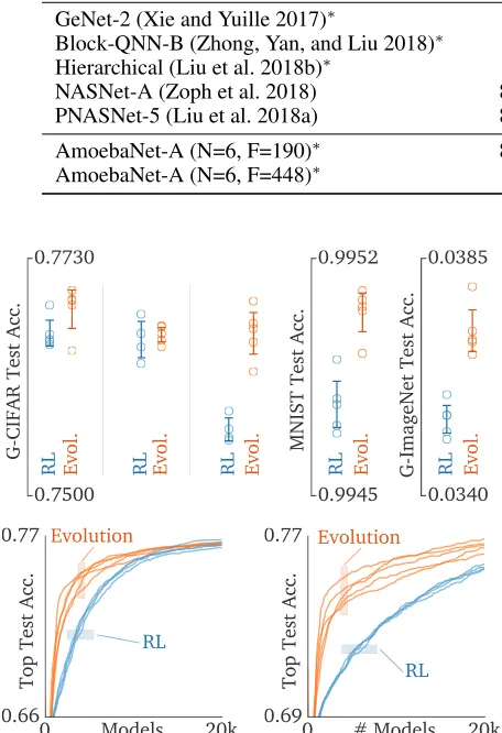
Scope of results.Some of our findings may be restricted to the search spaces and datasets we used. A natural direc-tion for future work is to extend the controlled comparison to more search spaces, datasets, and tasks, to verify general-ity, or to more algorithms. Supplement A presents prelimi-nary results, performing evolutioprelimi-nary and RL searches over three search spaces (SP-I: same as in the Results section; II: like I but with more possible ops; III: like SP-II but with more pairwise combinations) and three datasets (gray-scale CIFAR-10, MNIST, and gray-scale ImageNet), at a small-compute scale (on CPU, F=8,N=1). Evolution reached equal or better accuracy in all cases (Figure 7, top).

Algorithm speed.In our comparison study, Figure 4 sug-gested that both RL and evolution are approaching a com-mon accuracy asymptote. That raises the question of which algorithm gets there faster. The plots indicate that evolution reaches half-maximum accuracy in roughly half the time. We abstain, nevertheless, from further quantifying this ef-fect since it depends strongly on how speed is measured (the number of models necessary to reach accuracyadepends on

a; the natural choice ofa =amax/2may be too low to be

Table 2: ImageNet classification results for AmoebaNet-A compared to hand-designs (top rows) and other automated methods (middle rows). The evolved AmoebaNet-A architecture (bottom rows) reaches the current state of the art (SOTA) at similar model sizes and sets a new SOTA at a larger size. All evolution-based approaches are marked with a∗. We omitted Squeeze-and-Excite-Net because it was not benchmarked on the same ImageNet dataset version.

Model # Parameters # Multiply-Adds Top-1 / Top-5 Accuracy (%)

Incep-ResNet V2 (Szegedy et al. 2017) 55.8M 13.2B 80.4 / 95.3

ResNeXt-101 (Xie et al. 2017) 83.6M 31.5B 80.9 / 95.6

PolyNet (Zhang et al. 2017) 92.0M 34.7B 81.3 / 95.8

Dual-Path-Net-131 (Chen et al. 2017) 79.5M 32.0B 81.5 / 95.8

GeNet-2 (Xie and Yuille 2017)∗ 156M – 72.1 / 90.4

Block-QNN-B (Zhong, Yan, and Liu 2018)∗ – – 75.7 / 92.6

Hierarchical (Liu et al. 2018b)∗ 64M – 79.7 / 94.8

NASNet-A (Zoph et al. 2018) 88.9M 23.8B 82.7 / 96.2

PNASNet-5 (Liu et al. 2018a) 86.1M 25.0B 82.9 / 96.2

AmoebaNet-A (N=6, F=190)∗ 86.7M 23.1B 82.8 / 96.1

AmoebaNet-A (N=6, F=448)∗ 469M 104B 83.9 / 96.6

Figure 7: TOP: Comparison of the final model accuracy in five different contexts, from left to right: CIFAR/SP-I, CIFAR/SP-ICIFAR/SP-I, CIFAR/SP-IICIFAR/SP-I, MNIST/SP-I and G-ImageNet/SP-I. Each circle marks the top test accuracy at the end of one experiment. BOTTOM: Search progress of the experiments in the case of G-CIFAR/SP-II (LEFT, best for RL) and G-CIFAR/SP-III (RIGHT, best for evolution).

Model speed.The speed of individual models produced is also relevant. Figure 5 demonstrated that evolved models are faster (lower FLOPs). We speculate that asynchronous evo-lution may be reducing the FLOPs because it is indirectly optimizing for speed even when training for a fixed number of epochs: fast models may do well because they “repro-duce” quickly even if they initially lack the higher accuracy

of their slower peers. Verifying this speculation could be the subject of future work. As mentioned in the Related Work section, in this work we only considered asynchronous al-gorithms (as opposed to generational evolutionary methods) to ensure high resource utilization. Future work may ex-plore how asynchronous and generational algorithms com-pare with regard to model accuracy.

Benefits of aging evolution.Aging evolution also seemed advantageous in small-compute-scale experiments, shown in Figure 8 and presented in more detail in Supplement B.

Figure 8: Small-compute-scale comparison between our ag-ing tournament selection variant and the non-agag-ing variant, for different population sizes (P) and sample sizes (S). Ag-ing tends to be beneficial (most markers above the y=x line).

evolution tend to hold when varying the dataset or the search space. In order to reduce compute requirements, all these additional experiments were carried out on CPU instead of GPU and used a gray-scale version of CIFAR-10.

Understanding aging evolution and regularization.We can speculate that aging may help navigate the training noise in evolutionary experiments, as follows. Noisy training means that models may sometimes reach high accuracy just by luck. In non-aging evolution (NAE,i.e. standard tourna-ment selection), such lucky models may remain in the popu-lation for a long time—even for the whole experiment. One lucky model, therefore, can produce many children, caus-ing the algorithm to focus on it, reduccaus-ing exploration. Under aging evolution (AE), on the other hand, all models have a short lifespan, so the population is wholly renewed fre-quently, leading to more diversity and more exploration. In addition, another effect may be in play, which we describe next. In AE, because models die quickly, the only way an architecture can remain in the population for a long time is by being passed down from parent to child through the generations. Each time an architecture is inherited it must be trained. If it produces an inaccurate model when re-trained, that model is not selected by evolution and the ar-chitecture disappears from the population. The only way for an architecture to remain in the population for a long time is to re-train well repeatedly. In other words, AE can only im-prove a population through the inheritance of architectures that re-train well. (In contrast, NAE can improve a popu-lation by accumulating architectures/models that were lucky when they trained the first time). That is, AE is forced to pay attention toarchitecturesrather thanmodels. In other words, the addition of aging involves introducing additional infor-mation to the evolutionary process: architectures should re-train well. This additional information prevents overfitting to the training noise, which makes it a form of regulariza-tionin the broader mathematical sense1_{. Regardless of the}

exact mechanism, in Supplement C we perform experiments to verify the plausibility of the conjecture that aging helps navigate noise. There we construct a toy search space where the only difficulty is a noisy evaluation. If our conjecture is true, AE should be better in that toy space too. We found this to be the case. We leave further verification of the conjecture to future work, noting that theoretical results may prove use-ful here.

Simplicity of aging evolution.A desirable feature of evo-lutionary algorithms is their simplicity. By design, the appli-cation of a mutation causes a random change. The process of constructing new architectures, therefore, is entirely ran-dom. What makes evolution different from random search is that only the good models are selected to be mutated. This selection tends to improve the population over time. In this sense, evolution is simply “random search plus selection”. In outline, the process can be described briefly: “keep a popula-tion of N models and proceed in cycles: at each cycle, copy-mutate the best of S random models and kill the oldest in the population”. Implementation-wise, we believe the meth-ods of this paper are sufficient for a reader to understand

1

https://en.wikipedia.org/wiki/Regularization (mathematics)

evolution. The sophisticated nature of the RL alternative in-troduces complexity in its implementation: it requires back-propagation and poses challenges to parallelization (Sali-mans et al. 2017). Even different implementations of the same algorithm have been shown to produce different results (Henderson et al. 2018). Finally, evolution is also simple in that it has few meta-parameters, most of which do not need tuning (Real et al. 2017). In our study, we only adjusted 2 meta-parameters and only through a handful of attempts (see Methods Details section). In contrast, note that the RL base-line requires training an agent/controller which is often itself a neural network with many weights (such as an LSTM), and its optimization has more meta-parameters to adjust: learn-ing rate schedule, greediness, batchlearn-ing, replay buffer param-eters,etc. (These meta-parameters are all in addition to the weights and training parameters of the image classifiers be-ing searched, which are present in both approaches.) It is possible that through careful tuning, RL could be made to produce even better models than evolution, but such tun-ing would likely involve runntun-ing many experiments, mak-ing it more costly. Evolution did not require much tunmak-ing, as described. It is also possible that random search would produce equally good models if run for a very long time, which would be very costly. Finally, the evolutionary algo-rithm could be improved through additional complexity; for example, the mutation probabilities could be learned to im-prove speed.

Interpreting architecture search.Another important di-rection for future work is that of analyzing architecture-search experiments (regardless of the algorithm used) to try to discover new neural network design patterns. Anecdo-tally, for example, we found that architectures with high out-put vertex fan-in (number of edges into the outout-put vertex) tend to be favored in all our experiments. In fact, the mod-els in the final evolved populations have a mean fan-in value that is 3 standard deviations above what would be expected from randomly generated models. We verified this pattern by training various models with different fan-in values and the results confirm that accuracy increases with fan-in, as had been found in ResNeXt (Xie et al. 2017). Discovering broader patterns may require designing search spaces specif-ically for this purpose.

Additional AmoebaNets. Using variants of the evo-lutionary process described, we obtained three additional models, which we namedAmoebaNet-B,AmoebaNet-C, and

Supplements

Conclusion

This paper used an evolutionary algorithm to discover image classifier architectures. Our contributions are the following: • We proposedaging evolution, a variant of tournament se-lection by which genotypes die according to their age, fa-voring the young. This improved upon standard tourna-ment selection while still allowing for efficiency at scale through asynchronous population updating. We open-sourced the code.2 _{We also implemented simple}

muta-tions that permit the application of evolution to the popu-lar NASNet search space.

• We presented the first controlled comparison of algo-rithms for image classifier architecture search in a case study of evolution, RL and random search. We showed that evolution had somewhat faster search speed and stood out in the regime of scarcer resources / early stopping. Evolution also matched RL in final model quality, em-ploying a simpler method.

• We evolved AmoebaNet-A (Figure 6), a competitive im-age classifier. On Imim-ageNet, it is the first evolved model to surpass hand-designs. Matching size, AmoebaNet-A has comparable accuracy to top image-classifiers discov-ered with other architecture-search methods. At large size, it sets a new state-of-the-art accuracy. We open-sourced code and checkpoint.3

Acknowledgments

We wish to thank Megan Kacholia, Vincent Vanhoucke, Xi-aoqiang Zheng and especially Jeff Dean for their support and valuable input; Chris Ying for his work helping tune AmoebaNet models and for his help with specialized hard-ware, Barret Zoph and Vijay Vasudevan for help with the code and experiments used in their paper (Zoph et al. 2018), as well as Jiquan Ngiam, Jacques Pienaar, Arno Eigenwillig, Jianwei Xie, Derek Murray, Gabriel Bender, Golnaz Ghiasi, Saurabh Saxena and Jie Tan for other coding contributions; Jacques Pienaar, Luke Metz, Chris Ying, Andrew Selle and the anonymous reviewers for manuscript comments, all the above and Patrick Nguyen, Samy Bengio, Geoffrey Hinton, Risto Miikkulainen, Jeff Clune, Kenneth Stanley, Yifeng Lu, David Dohan, David So, David Ha, Vishy Tirumalashetty, Yoram Singer, and Ruoming Pang for helpful discussions; and the larger Google Brain team.

References

Angeline, P. J.; Saunders, G. M.; and Pollack, J. B. 1994. An evolutionary algorithm that constructs recurrent neural networks. IEEE transactions on Neural Networks.

2

https://colab.research.google.com/github/google-research/ google-research/blob/master/evolution/regularized evolution algorithm/regularized evolution.ipynb

3

https://tfhub.dev/google/imagenet/amoebanet a n18 f448/ classification/1

Baker, B.; Gupta, O.; Naik, N.; and Raskar, R. 2017a. Designing neural network architectures using reinforcement learning. InICLR.

Baker, B.; Gupta, O.; Raskar, R.; and Naik, N. 2017b. Ac-celerating neural architecture search using performance pre-diction. ICLR Workshop.

Bergstra, J., and Bengio, Y. 2012. Random search for hyper-parameter optimization.JMLR.

Brock, A.; Lim, T.; Ritchie, J. M.; and Weston, N. 2018. Smash: one-shot model architecture search through hyper-networks. InICLR.

Cai, H.; Chen, T.; Zhang, W.; Yu, Y.; and Wang, J. 2018. Efficient architecture search by network transformation. In

AAAI.

Chen, Y.; Li, J.; Xiao, H.; Jin, X.; Yan, S.; and Feng, J. 2017. Dual path networks. InNIPS.

Ciregan, D.; Meier, U.; and Schmidhuber, J. 2012. Multi-column deep neural networks for image classification. In

CVPR.

Coleman, C.; Kang, D.; Narayanan, D.; Nardi, L.; Zhao, T.; Zhang, J.; Bailis, P.; Olukotun, K.; Re, C.; and Zaharia, M. 2018. Analysis of dawnbench, a time-to-accuracy machine learning performance benchmark. arXiv preprint arXiv:1806.01427.

Cortes, C.; Gonzalvo, X.; Kuznetsov, V.; Mohri, M.; and Yang, S. 2017. Adanet: Adaptive structural learning of arti-ficial neural networks. InICML.

Cubuk, E. D.; Zoph, B.; Mane, D.; Vasudevan, V.; and Le, Q. V. 2018. Autoaugment: Learning augmentation policies from data. arXiv.

Deng, J.; Dong, W.; Socher, R.; Li, L.-J.; Li, K.; and Fei-Fei, L. 2009. Imagenet: A large-scale hierarchical image database. InCVPR.

Domhan, T.; Springenberg, J. T.; and Hutter, F. 2017. Speed-ing up automatic hyperparameter optimization of deep neu-ral networks by extrapolation of learning curves. InIJCAI. Elsken, T.; Metzen, J.-H.; and Hutter, F. 2017. Simple and efficient architecture search for convolutional neural net-works. ICLR Workshop.

Elsken, T.; Metzen, J. H.; and Hutter, F. 2018. Neural archi-tecture search: A survey. arXiv.

Fahlman, S. E., and Lebiere, C. 1990. The cascade-correlation learning architecture. InNIPS.

Feurer, M.; Klein, A.; Eggensperger, K.; Springenberg, J.; Blum, M.; and Hutter, F. 2015. Efficient and robust auto-mated machine learning. InNIPS.

Floreano, D.; D¨urr, P.; and Mattiussi, C. 2008. Neuroevo-lution: from architectures to learning. Evolutionary Intelli-gence.

Henderson, P.; Islam, R.; Bachman, P.; Pineau, J.; Precup, D.; and Meger, D. 2018. Deep reinforcement learning that matters.AAAI.

Hornby, G. S. 2006. Alps: the age-layered population struc-ture for reducing the problem of premastruc-ture convergence. In

GECCO.

Hu, J.; Shen, L.; and Sun, G. 2018. Squeeze-and-excitation networks. CVPR.

Huang, G.; Liu, Z.; Weinberger, K. Q.; and van der Maaten, L. 2017. Densely connected convolutional networks. In

CVPR.

Klein, A.; Falkner, S.; Springenberg, J. T.; and Hutter, F. 2017. Learning curve prediction with bayesian neural net-works.ICLR.

Krizhevsky, A., and Hinton, G. 2009. Learning multiple layers of features from tiny images. Master’s thesis, Dept. of Computer Science, U. of Toronto.

Krizhevsky, A.; Sutskever, I.; and Hinton, G. E. 2012. Imagenet classification with deep convolutional neural net-works. InNIPS.

Liu, C.; Zoph, B.; Shlens, J.; Hua, W.; Li, L.-J.; Fei-Fei, L.; Yuille, A.; Huang, J.; and Murphy, K. 2018a. Progressive neural architecture search. ECCV.

Liu, H.; Simonyan, K.; Vinyals, O.; Fernando, C.; and Kavukcuoglu, K. 2018b. Hierarchical representations for efficient architecture search. InICLR.

Mendoza, H.; Klein, A.; Feurer, M.; Springenberg, J. T.; and Hutter, F. 2016. Towards automatically-tuned neural net-works. InWorkshop on Automatic Machine Learning. Miikkulainen, R.; Liang, J.; Meyerson, E.; Rawal, A.; Fink, D.; Francon, O.; Raju, B.; Navruzyan, A.; Duffy, N.; and Hodjat, B. 2017. Evolving deep neural networks.arXiv. Miller, G. F.; Todd, P. M.; and Hegde, S. U. 1989. Designing neural networks using genetic algorithms. InICGA. Negrinho, R., and Gordon, G. 2017. Deeparchitect: Auto-matically designing and training deep architectures.arXiv. Pham, H.; Guan, M. Y.; Zoph, B.; Le, Q. V.; and Dean, J. 2018. Faster discovery of neural architectures by searching for paths in a large model.ICLR Workshop.

Real, E.; Moore, S.; Selle, A.; Saxena, S.; Suematsu, Y. L.; Le, Q.; and Kurakin, A. 2017. Large-scale evolution of image classifiers. InICML.

Salimans, T.; Ho, J.; Chen, X.; and Sutskever, I. 2017. Evo-lution strategies as a scalable alternative to reinforcement learning.arXiv.

Saxena, S., and Verbeek, J. 2016. Convolutional neural fab-rics. InNIPS.

Simmons, J. P.; Nelson, L. D.; and Simonsohn, U. 2011. False-positive psychology: Undisclosed flexibility in data collection and analysis allows presenting anything as sig-nificant.Psychological Science.

Srivastava, N.; Hinton, G.; Krizhevsky, A.; Sutskever, I.; and Salakhutdinov, R. 2014. Dropout: A simple way to prevent neural networks from overfitting.JMLR.

Stanley, K. O., and Miikkulainen, R. 2002. Evolving neural networks through augmenting topologies. Evol. Comput.

Stanley, K. O.; Bryant, B. D.; and Miikkulainen, R. 2005. Real-time neuroevolution in the nero video game.TEVC. Suganuma, M.; Shirakawa, S.; and Nagao, T. 2017. A genetic programming approach to designing convolutional neural network architectures. InGECCO.

Szegedy, C.; Liu, W.; Jia, Y.; Sermanet, P.; Reed, S.; Anguelov, D.; Erhan, D.; Vanhoucke, V.; and Rabinovich, A. 2015. Going deeper with convolutions. InCVPR. Szegedy, C.; Ioffe, S.; Vanhoucke, V.; and Alemi, A. A. 2017. Inception-v4, inception-resnet and the impact of resid-ual connections on learning. InAAAI.

Wan, L.; Zeiler, M.; Zhang, S.; Le Cun, Y.; and Fergus, R. 2013. Regularization of neural networks using dropconnect. InICML.

Xie, L., and Yuille, A. 2017. Genetic CNN. InICCV. Xie, S.; Girshick, R.; Doll´ar, P.; Tu, Z.; and He, K. 2017. Ag-gregated residual transformations for deep neural networks. InCVPR.

Yao, X. 1999. Evolving artificial neural networks. IEEE. Zagoruyko, S., and Komodakis, N. 2016. Wide residual networks. InBMVC.

Zhang, X.; Li, Z.; Loy, C. C.; and Lin, D. 2017. Polynet: A pursuit of structural diversity in very deep networks. In

CVPR.

Zhong, Z.; Yan, J.; and Liu, C.-L. 2018. Practical network blocks design with q-learning. InAAAI.

Zoph, B., and Le, Q. V. 2016. Neural architecture search with reinforcement learning. InICLR.