Technological Change and its Relationship with Total Factor Productivity in Iran's Petroleum Refineries

(1)

P

etroleum

B

usiness

R

eview

22

Technological Change and its Relationship

with Total Factor Productivity

in Iran's Petroleum Refineries

Nader Dashtia*_{, Mahdi Rostami}b_{, Reza Rashidi}c

a

_{Assistant Professor,Energy Economics and Management Department,Petroleum Faculty of Tehran, Petroleum University of Technology}

, Iran, Email: [email protected]

b

_{Assistant Professor,Energy Economics and Management Department,Petroleum Faculty of Tehran, Petroleum University of Technology}

, Iran, Email: [email protected]

c

_{MA Student in Oil & Gas Economics, Petroleum Faculty of Tehran, Petroleum University of Technology, Iran, Email:[email protected]}

Nowadays, using appropriate technologies in order to increase productivity of production factors can be resulted in optimal factors employment and production enhancement in factories. Technological change is considered as one of the main sources of productivity growth. The purpose of this paper is to analyze the various aspects of technological change and their relationship with total factor productivity in Iran’s petroleum refineries.

In order to achieve this goal, we used the econometric method to estimate the cost function. This method seems useful to estimate the structure of fac-tors demand, considering changes in facfac-tors prices and technology status. We estimated a translog cost function as well as equations system of cost share, using Seemingly Unrelated Regressions (SUR) approach from 1982 to 2012.

The results show that the average rate of technological change was -0.482 percent over the study period. It means that over time, the cost growth rate of production units was decreased mainly due to technological change. Fur-thermore, the results indicate that technological change was biased towards the use of more labor and material, while it saved more capital and energy. Also, based on the estimation results, we decomposed total factor produc-tivity growth rate into the contributions of technological change and econo-mies of scale. Decomposition results show that the share of technological change in the productivity growth is greater than that of scale economies. A B S T R A C T

Keywords:

Productivity

Technological change Translog cost function, Petroleum refineries A R T I C L E I N F O

Received: 04.Apr.2017

Received in revised: 13.Aug.2017 Accepted: 19.Aug.2017

1. Introduction

Petroleum Refineries are considered as one of the most important parts of the oil industry value chain. This sector operates as an important tool for linking between the up-stream production and consumer market.

Iran is a major producer of oil, but the country is rela-tively weak on petroleum refining capacity. Although the number of oil refineries was increased but for many reasons including low technology, resources were not been used ef-ficiently and as a result many potential capacities of the re -fineries have not been utilized.

(2)

Volume 1, Issue 1

November 2017

23

studies on technical change were expanded in economics. Some of the well-known studies are Solow (1957, 1962), Salter (1960), Intriligator (1965), McCarthy (1965), Dranda-kis and Phelps (1966) Jorgenson (1966), Nordhaus (1969), Atkinson and Stiglitz (1969), Diewert (1971), Binswanger (1974), Stevenson (1980), Romer (1990), Kant and Nautiyal (1997), Peretto (1999), Rasmussen (2000), Napasintuwong and Emerson (2002,2003), Datta and Christoffersen (2004), Grebel (2009), Krysiak (2011), Mattalia (2013), Hart (2013), Roshef (2013), Schafer (2014), and Chen and Wemy (2015) among others.

Tendency toward such researches have two main rea-sons: Firstly, supply increase of industrial products versus their demand caused decreasing trend in their prices and consequently in industrial section’s revenue. This attracted many economists to discover the reasons of the growth, and they found that one of the main reasons for such growth is technical change. Secondly, there was a shortage of indus-trial materials in developing countries. Therefore, according to the aforesaid studies, technical change was considered as a major reason of productivity growth (Hayami and Godo, 2005).

Technological change in petroleum refineries is also one of the main elements of productivity growth. Thus, it is nec-essary to enhance our understandings on the technology of petroleum refineries, bias and rate of growth in order to mod -ify and improve the industry condition. Considering above, the main purpose of this study is to analyze different aspects of technological change in Iran’s petroleum refineries during the years 1982-2012.

2. Methodology

In production process literature, production technology is defined as the relation between inputs and output, which can be illustrated by production function (Chambers, 1988). The production structure and technological change can be surveyed by production function or dual cost function. Di-rect estimation of production function will be appropriate if amount of output is determined endogenously, while for exogenous amount of output cost function is preferred (Kant and Nautiyal, 1997).

For this study we chose translog functional form as the most appropriate functional form among all functional forms, because it is widely used in similar researches and also is flexible enough. Furthermore, it has several theo -retical and statistical characteristics advantages such as the

flexibility of avoiding pre-specification of any particular re -lationships, and the imposition of minimum restrictions on the parameters. Moreover, factor demand functions can be derived from Shepherd’s lemma (Bhattacharyya, 2011).

General form of cost function considering time trend (T) variable is as follow (Rasmussen, 2000):

(1)

2

were expanded in economics. Some of the well-known studies are Solow (1957, 1962), Salter

(1960), Intriligator (1965), McCarthy (1965), Drandakis and Phelps (1966) Jorgenson (1966),

Nordhaus (1969), Atkinson and Stiglitz (1969), Diewert (1971), Binswanger (1974), Stevenson

(1980), Romer (1990), Kant and Nautiyal (1997), Peretto (1999), Rasmussen (2000),

Napasintuwong and Emerson (2002,2003), Datta and Christoffersen (2004), Grebel (2009),

Krysiak (2011), Mattalia (2013), Hart (2013), Roshef (2013), Schafer (2014), and Chen and

Wemy (2015) among others.

Tendency toward such researches have two main reasons: Firstly, supply increase of industrial

products versus their demand caused decreasing trend in their prices and consequently in industrial

section’s revenue. This attracted many economists to discover the reasons of the growth, and they

found that one of the main reasons for such growth is technical change. Secondly, there was a

shortage of industrial materials in developing countries. Therefore, according to the aforesaid

studies, technical change was considered as a major reason of productivity growth (Hayami and

Godo, 2005).

Technological change in petroleum refineries is also one of the main elements of productivity

growth. Thus, it is necessary to enhance our understandings on the technology of petroleum

refineries, bias and rate of growth in order to modify and improve the industry condition.

Considering above, the main purpose of this study is to analyze different aspects of technological

change in Iran’s petroleum refineries during the years 1982-2012.

2. Methodology

In production process literature, production technology is defined as the relation between inputs

and output, which can be illustrated by production function (Chambers, 1988). The production

structure and technological change can be surveyed by production function or dual cost function.

Direct estimation of production function will be appropriate if amount of output is determined

endogenously, while for exogenous amount of output cost function is preferred (Kant and Nautiyal,

1997).

For this study we chose translog functional form as the most appropriate functional form among

all functional forms, because it is widely used in similar researches and also is flexible enough.

Furthermore, it has several theoretical and statistical characteristics advantages such as the

flexibility of avoiding pre-specification of any particular relationships, and the imposition of

minimum restrictions on the parameters. Moreover, factor demand functions can be derived from

Shepherd’s lemma (Bhattacharyya, 2011).

General form of cost function considering time trend (T) variable is as follow (Rasmussen,

2000):

C = f (P

l

, P

k

, P

e

, P

m

, Q, T)

(1)

In which P

l

, P

k

, P

e

and P

m

are prices of labor, capital, energy and material respectively. Q is

value of product and C is cost. So, translog cost function is written as follow:

In which Pl, Pk, Pe and Pm are prices of labor, capital, energy and material respectively. Q is value of product and C is cost. So, translog cost function is written as follow:

(2) 3





 









m e l k j i T Q b T P b T b T b Q b P LnQ b LnP LnP b Q a LnP a v C Ln qt i i ti

i iq i q t tt

i j ij i j

i i i q

, , , , ln ln 2 1 ln 2 1 ln 2 1 ln 2 2           







(2)

Factor cost shares can be obtained by partial derivation of translog function with respect to i-th input price, thus:

i i i i i i S C P x C P P C P

C _ _

     ln ln (3)



   

j ij j iq ti

i

i a b P b Q bT

S ln ln

(4)

In which, C



PiXi_{, S}_i_{is cost share of i-th input and X refers to amount of factor.}

In order to ensure that the underlying cost function is well-behaved, the cost function must be homogeneous of degree one in input prices, given output. Then, liner homogeneity in factor prices and symmetry imposes the following restrictions:



  j ij j i b

a 1 0



biq0 bij bji₍₅₎

Rate of technological change can be obtained by derivation of cost function with respect to time (Datta and Christoffersen, 2004 and Kant and Nautiyal, 1997):

(3) 3         m e l k j i T Q b T P b T b T b Q b P LnQ b LnP LnP b Q a LnP a v C Ln qt i i ti

i iq i q t tt

i j ij i j

i i i q

, , , , ln ln 2 1 ln 2 1 ln 2 1 ln 2 2           







(2)

C _ _

     ln ln (3)



   

j ij j iq ti

i

i a b P b Q bT

S ln ln

(4)

In which, C



  j ij j i b

a 1 0



biq0 bij bji₍₅₎

(4) 3





 









m e l k j i T Q b T P b T b T b Q b P LnQ b LnP LnP b Q a LnP a v C Ln qt i i ti

i iq i q t tt

i j ij i j

i i i q

, , , , ln ln 2 1 ln 2 1 ln 2 1 ln 2 2           







(2)

C _ _

    

lnln ₍₃₎



 

 

j ij j iq ti

i

i a b P b Q bT

S ln ln

(4)

In which, C



  j ij j i b

a 1 0



biq0 bij bji₍₅₎

In which, 3         m e l k j i T Q b T P b T b T b Q b P LnQ b LnP LnP b Q a LnP a v C Ln qt i i ti

i iq i q t tt

i j ij i j

i i i q

, , , , ln ln 2 1 ln 2 1 ln 2 1 ln 2 2           







(2)

C _ _

     ln ln (3)



   

j ij j iq ti i

i a b P b Q bT

S ln ln

(4)

In which, C



  j ij j i b

a 1 0



biq0 bijbji₍₅₎

, Si is cost share of i-th input and X refers to amount of factor.

In order to ensure that the underlying cost function is well-behaved, the cost function must be homogeneous of degree one in input prices, given output. Then, liner homo-geneity in factor prices and symmetry imposes the following restrictions: (5) 3         m e l k j i T Q b T P b T b T b Q b P LnQ b LnP LnP b Q a LnP a v C Ln qt i i ti

i iq i q t tt

i j ij i j i i i q

, , , , ln ln 2 1 ln 2 1 ln 2 1 ln 2 2                (2)

C _ _

     ln ln (3)     

j ij j iq ti i

i a b P b Q bT

S ln ln

(4)

In which, CPiXi_{, S}_i_{is cost share of i-th input and X refers to amount of factor.} In order to ensure that the underlying cost function is well-behaved, the cost function must be homogeneous of degree one in input prices, given output. Then, liner homogeneity in factor prices and symmetry imposes the following restrictions:

    j ij j i b

a 1 0



biq0 bij bji₍₅₎

Rate of technological change can be obtained by derivation of cost function with respect to time (Datta and Christoffersen, 2004 and Kant and Nautiyal, 1997): _{tion of cost function with respect to time (Datta and Christof-}Rate of technological change can be obtained by

deriva-fersen, 2004 and Kant and Nautiyal, 1997):

(6)

4

T b bT b P b Q C

C_ln ttt 



tilniqtln



(6)

It shows that technological change can be divided into three elements: 1- pure technical change (bt+btt T)

2- non-neutral technical change (btilnPi)

3- scale-augmenting technical change (bqt lnQ)

The first element – pure technical change- has no relation with inputs, amount of output and factor prices. It is a fixed part of function and its change causes cost function moving towards up or down. If it is negative, cost function goes down and it indicates positive technological change.

Interaction of factors over time is in second element. In other words, it shows the effects of technological change on factors during the time. It shows any substitution or saving factors. Changing this element results slope changing of cost curve.

Third element is the effect of technological change on the capacity of institute. Clearly scale-augmenting technological change causes Economies of scale, due to increasing in production. It also decreases cost and leads to cost function shift.In cost function, return to scale (scale elasticity) is determined as follow:

1 1 ln ln ln

ln  _

     _ _ _         

 a b Q b P bT Q

C

E i qt

i iq q q

(7)

Return to scale refers to changes in output subsequent to a proportional change in all inputs (where all inputs increase by a constant factor). If output increases by that same proportional change then there are constant returns to scale (CRS). If output increases by less than that proportional change, there are decreasing returns to scale (DRS). If output increases by more than that proportion, there are increasing returns to scale (IRS).

Stevenson (1980) believes that technological change may have bias to factor and scale characteristics of production. In case of technical progress, factor bias is as follow:

It shows that technological change can be divided into three elements:

1- pure technical change (bt+btt T) 2- non-neutral technical change (

4

T

b

T

b

P

b

Q

C

_

ln



t



tt



ti

ln

i



qt

ln









(6)

It shows that technological change can be divided into three elements:

1-

pure technical change (b

t

+b

tt

T)

2-

non-neutral technical change (

btilnPi

)

3-

scale-augmenting technical change (b

qt

lnQ)

The first element – pure technical change- has no relation with inputs, amount of output and factor

prices. It is a fixed part of function and its change causes cost function moving towards up or down.

If it is negative, cost function goes down and it indicates positive technological change.

Interaction of factors over time is in second element. In other words, it shows the effects of

technological change on factors during the time. It shows any substitution or saving factors.

Changing this element results slope changing of cost curve.

Third element is the effect of technological change on the capacity of institute. Clearly

scale-augmenting technological change causes Economies of scale, due to increasing in production. It

also decreases cost and leads to cost function shift.In cost function, return to scale (scale elasticity)

is determined as follow:

1 1 ln ln ln

ln  _

     _ _ _         

 a b Q



b P bT

Q C

E i qt

i iq q

q

(7)

Return to scale refers to changes in output subsequent to a proportional change in all inputs (where

all inputs increase by a constant factor). If output increases by that same proportional change then

there are constant returns to scale (CRS). If output increases by less than that proportional change,

there are decreasing returns to scale (DRS). If output increases by more than that proportion, there

are increasing returns to scale (IRS).

Stevenson (1980) believes that technological change may have bias to factor and scale

characteristics of production. In case of technical progress, factor bias is as follow:

) 3- scale-augmenting technical change (bqt lnQ)

(3)

P

etroleum

B

usiness

R

eview

24

with inputs, amount of output and factor prices. It is a fixed part of function and its change causes cost function mov-ing towards up or down. If it is negative, cost function goes down and it indicates positive technological change.

Third element is the effect of technological change on the capacity of institute. Clearly scale-augmenting techno-logical change causes Economies of scale, due to increasing in production. It also decreases cost and leads to cost func-tion shift.In cost funcfunc-tion, return to scale (scale elasticity) is determined as follow:

(7)

4

T b bT b P b Q

C

C_ln  t tt 



tilni qtln



(6)

It shows that technological change can be divided into three elements:

1- pure technical change (bt+btt T)

2- non-neutral technical change (btilnPi)

3- scale-augmenting technical change (bqt lnQ)

The first element – pure technical change- has no relation with inputs, amount of output and factor prices. It is a fixed part of function and its change causes cost function moving towards up or down. If it is negative, cost function goes down and it indicates positive technological change.

Third element is the effect of technological change on the capacity of institute. Clearly scale-augmenting technological change causes Economies of scale, due to increasing in production. It also decreases cost and leads to cost function shift.In cost function, return to scale (scale elasticity) is determined as follow:

1 1

ln ln ln

ln  _

  



 _ _ _

        

 a b Q



b P bT

Q C

E i qt

i iq

q q

(7)

Return to scale refers to changes in output subsequent to a proportional change in all inputs (where all inputs increase by a constant factor). If output increases by that same proportional change then there are constant returns to scale (CRS). If output increases by less than that proportional change, there are decreasing returns to scale (DRS). If output increases by more than that proportion, there are increasing returns to scale (IRS).

Stevenson (1980) believes that technological change may have bias to factor and scale characteristics of production. In case of technical progress, factor bias is as follow:

Return to scale refers to changes in output subsequent to a proportional change in all inputs (where all inputs in-crease by a constant factor). If output inin-creases by that same proportional change then there are constant returns to scale (CRS). If output increases by less than that proportional change, there are decreasing returns to scale (DRS). If output increases by more than that proportion, there are increasing returns to scale (IRS).

Stevenson (1980) believes that technological change may have bias to factor and scale characteristics of produc-tion. In case of technical progress, factor bias is as follow:

(8)

5

T S

I i

bi_

(8)

If I

bi>

0, technological change results to use input i more. If I

bi

<0, technological change saves input

i. If I

bi

=0 then it has no effect on using input i. Scale bias is calculated by derivation of the phrase

in bracket:

Q

S

Q

P

C

SE

i

_ln

ln

_ln

2













(9)

If SE

i

>0, increasing of production scale, leads to use input i more. If SE

i

<0, it leads to use input i

less. If SE

i

=0 it has no effect on using input i.

Cost function system can be estimated if data and information is available. Although parameters

of basic cost function are being estimated by Ordinary Least Squares (OLS) method, but it does

not include cost share equations. A suitable method to estimate such systems is Seemingly

Unrelated Regression (SUR). Since value shares sum to using, the sum of the disturbances across

any three equations is zero at all observations (Baltagi, 2005). Hence, to avoid singularity of the

covariance matrix any one of the four share equations can be dropped, i.e., three can be estimated

and the forth is automatically determined (Kant and Nautiyal, 1997). We drop energy share

equation. Eventually, according to the methodology, technological change is being analyzed.

3. Technological change and total factor productivity

There are different ways to calculate the total factor productivity

.

In this research this criterion

calculated through econometric method and estimation of parameters. In this way, by estimating

cost elasticity of the relevant production and replacing it in the following formula, total factor

productivity growth can be estimated (Baltagi and Griffin, 1988):

 



Q

T

TFP







(

1 



CQ

)

₍₁₀₎

If Ibi<0, technological change results to use input i more. If Ibi<0, technological change saves input i. If Ibi=0 then it has no effect on using input i. Scale bias is calculated by deriva-tion of the phrase in bracket:

(9)

5 T

S

I i

bi_

(8)

If Ibi>0, technological change results to use input i more. If Ibi<0, technological change saves input i. If Ibi=0 then it has no effect on using input i. Scale bias is calculated by derivation of the phrase in bracket:

Q S Q P

C

SE i

i

i _ln _ln _ln

ln 2

     

 

(9)

If SEi>0, increasing of production scale, leads to use input i more. If SEi<0, it leads to use input i less. If SEi=0 it has no effect on using input i.

Cost function system can be estimated if data and information is available. Although parameters of basic cost function are being estimated by Ordinary Least Squares (OLS) method, but it does not include cost share equations. A suitable method to estimate such systems is Seemingly Unrelated Regression (SUR). Since value shares sum to using, the sum of the disturbances across any three equations is zero at all observations (Baltagi, 2005). Hence, to avoid singularity of the covariance matrix any one of the four share equations can be dropped, i.e., three can be estimated and the forth is automatically determined (Kant and Nautiyal, 1997). We drop energy share equation. Eventually, according to the methodology, technological change is being analyzed.

3. Technological change and total factor productivity

There are different ways to calculate the total factor productivity. In this research this criterion calculated through econometric method and estimation of parameters. In this way, by estimating cost elasticity of the relevant production and replacing it in the following formula, total factor productivity growth can be estimated (Baltagi and Griffin, 1988):

 



Q T

TFP (1CQ) ₍₁₀₎

If SEi>0, increasing of production scale, leads to use in-put i more. If SEi<0, it leads to use inin-put i less. If SEi=0 it has no effect on using input i.

Cost function system can be estimated if data and infor-mation is available. Although parameters of basic cost func-tion are being estimated by Ordinary Least Squares (OLS) method, but it does not include cost share equations. A suit-able method to estimate such systems is Seemingly Unre-lated Regression (SUR). Since value shares sum to using,

the sum of the disturbances across any three equations is zero at all observations (Baltagi, 2005). Hence, to avoid sin-gularity of the covariance matrix any one of the four share equations can be dropped, i.e., three can be estimated and the forth is automatically determined (Kant and Nautiyal, 1997). We drop energy share equation. Eventually, according to the methodology, technological change is being analyzed.

3. Technological change and total factor

pro-ductivity

There are different ways to calculate the total factor pro-ductivity. In this research this criterion calculated through econometric method and estimation of parameters. In this way, by estimating cost elasticity of the relevant production and replacing it in the following formula, total factor produc-tivity growth can be estimated (Baltagi and Griffin, 1988):

(10)

5

T S

I i

bi_

(8)

If Ibi>0, technological change results to use input i more. If Ibi<0, technological change saves input

i. If Ibi=0 then it has no effect on using input i. Scale bias is calculated by derivation of the phrase

in bracket:

Q S Q P

C

SE i

i i

ln ln

2

     

 

(9)

If SEi>0, increasing of production scale, leads to use input i more. If SEi<0, it leads to use input i

less. If SEi=0 it has no effect on using input i.

Cost function system can be estimated if data and information is available. Although parameters of basic cost function are being estimated by Ordinary Least Squares (OLS) method, but it does not include cost share equations. A suitable method to estimate such systems is Seemingly Unrelated Regression (SUR). Since value shares sum to using, the sum of the disturbances across any three equations is zero at all observations (Baltagi, 2005). Hence, to avoid singularity of the covariance matrix any one of the four share equations can be dropped, i.e., three can be estimated and the forth is automatically determined (Kant and Nautiyal, 1997). We drop energy share equation. Eventually, according to the methodology, technological change is being analyzed.

3. Technological change and total factor productivity

There are different ways to calculate the total factor productivity. In this research this criterion

calculated through econometric method and estimation of parameters. In this way, by estimating cost elasticity of the relevant production and replacing it in the following formula, total factor productivity growth can be estimated (Baltagi and Griffin, 1988):

 



Q T

TFP (1CQ) ₍₁₀₎

In this regard,

6

In this regard,T indicates the technological change,



CQ_{is elasticity of the}_{cost related to product,}



Q_{is the per cent of production growth.}

4. Sources of Data and Structure of Variables

The data were collected from various editions of the Iranian reports on industrial enterprises and different volume of the Wholesale Price Index in Iran. We have adopted 2004 as base year to converting nominal data to real data. Output is the value of aggregate output produced during the year. This implies that no change in the stock of output has taken place. The capital expenditure is computed as the user cost of capital multiplied by the capital stock. In order to calculate the user cost of capital, we used Puk=(r+P) Pi, where r is the long run interest rate, P is the depreciated rate of capital assumed to be 5.5 % by year and Pi is the investment deflator.

Total cost is the sum of the cost of labor, capital, material and energy. For labor input, the number of persons employed and the wage calculated for emoluments per person employed have been used for model estimation. The price of labor is obtained as the ratio of total compensation to labor divided by the number of workers. Fuel cost is the cost of all types of fuel used for production. We add fuel cost to electricity cost to obtain energy cost. The price of fuel is obtained by taking a weighted average of all types of fuel prices. The price of energy is obtained by taking a weighted average of fuel and electricity price. The cost share of labor, capital, material and energy are obtained by dividing the corresponding cost by the total cost.

5. Test of Stationarity

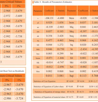
To use time series data in estimation of model, we need to examine the series for stationarity. If a time series is stationary, its mean, variance, and autocovariance (at various lags) remain the same no matter at what point we measure them; that is, they are time invariant. If series are nonstationary, F and t statistics are not valid and estimated model is not reliable (Gujarati, 2004). A commonly used test that is valid in large samples is the Augmented Dickey–Fuller test. Results of the Augmented Dickey-Fuller (ADF) test showed that all variables have unit root and after first difference ADF statistics were greater than Mackinnon Critical Values and thus we can reject the null hypothesis of a unit root at all common significance levels which means they become stationary (Table 1). Also the test shows stationarity of residuals (table 2). Thus, spurious regression is rejected and the results of estimation are reliable.

indicates the technological change,is

6



CQ_{is elasticity of the}_{cost related to product,} 

elasticity of the cost related to product,

6



CQ_{is elasticity of the}_{cost related to product,}



is the per cent of production growth.

4. Sources of Data and Structure of Variables

(4)

Volume 1, Issue 1

November 2017

25

fuel and electricity price. The cost share of labor, capital, ma-terial and energy are obtained by dividing the corresponding cost by the total cost.

5. Test of Stationarity

To use time series data in estimation of model, we need to examine the series for stationarity. If a time series is sta-tionary, its mean, variance, and autocovariance (at various lags) remain the same no matter at what point we measure them; that is, they are time invariant. If series are nonstation-ary, F and t statistics are not valid and estimated model is not reliable (Gujarati, 2004). A commonly used test that is valid in large samples is the Augmented Dickey–Fuller test.

Results of the Augmented Dickey-Fuller (ADF) test showed that all variables have unit root and after first dif -ference ADF statistics were greater than Mackinnon Critical Values and thus we can reject the null hypothesis of a unit root at all common significance levels which means they be -come stationary (Table 1). Also the test shows stationarity of residuals (table 2). Thus, spurious regression is rejected and

the results of estimation are reliable.

6. Empirical Results

6.1 Parameter estimates of the translog cost

function

The parameter estimates of the translog cost function along with the associated cost share equations are presented in Table 3. Many significant variables and high value of R2 are signs of good estimation. Durbin Watson (D.W) statistic shows that there is no autocorrelation in the estimated model.

6.2 Rate of Technological Change

The study of technological change over the study years clarified that by the passage of time, technological progress in petrochemical industry decreased the rate of cost change. According to the equation 6, rate of technological change since 1982 to 2012 was -0.482. It means that average rate of decrease in cost of production was 0.482 % each year. As Table 4 portrays, although this rate changes over time, but negative sign means decreasing in cost rate during the time. Thus, our estimations confirm that technological progress decreased rate of cost change of the petroleum refineries.

Mackinnon Critical Values

ADF statistics Variable*

1% 5%

10%

-3.679 -2.968

-2.623 -5.325

D(LC)

-3.689 -2.972

-2.625 -5.081

D(LPL)

-3.679 -2.968

-2.623 -3.853

D(LPK)

-3.679 -2.968

-2.623 -4.674

D(LPE)

-3.679 -2.968

-2.623 -4.003

D(KPM)

-3.738 -2.992

-2.636 -6.425

D(SL)

-3.679 -2.968

-2.623 -8.155

D(SK)

-3.679 -2.968

-2.623 -7.257

D(SE)

-3.679 -2.968

-2.623 -6.446

D(SM)

-3.679 -2.968

-2.623 -6.124

D(LQ)

* Ln of variables in equations no. 1 & 3

Table 1: Results of Augmented Dickey-Fuller Unit Root Test on Variables

Mackinnon Critical Values

ADF statistics Variable*

1% 5%

10%

-3.679 -2.967

-2.622 -6.306

RESID 1

-3.670 -2.963

-2.621 -3.938

RESID 2

-3.670 -2.963

-2.621 -5.334

RESID 3

-3.724 -2.986

-2.632 -4.408

RESID 4

Table 2: Results of Augmented Dickey-Fuller Unit Root Test on Residuals

Table 3: Results of Parameters Estimates

t- Statistic

Coefficient

Parameter t- Statistic

Coefficient

Parameter

-1.384 -0.028

bkm -4.480 -104.131

v

3.101 0.037

bem 1.838

0.929

al

2.463 0.041

blq -2.883 -0.339

ae

-10.114 -0.397

bkq 0.103 0.057

am

-1.370 -0.004

beq 3.428

0.354

ak

4.162 0.068

bmq 4.465

8.477

aq

0.283 0.020

bq 1.272 0.044

bll

-4.393 -2.434

bt 10.750 0.046

bkk

-3.145 -0.022

btt 0.299 0.003

bee

0.205 0.001

blt -1.446 -0.071

bmm

-1.857 -0.020

bkt -0.747 -0.014

blk

-1.850 -0.002

bet -2.696 -0.012

ble

0.419 0.002

bmt 0.068

0.002

blm

5.704 0.113

bqt 3.081 0.011

Statistics of Cost Equation R2_{=0.99 R}2_{=0.94 D.W=2.17}

Statistics of Equation of Labor share R2_{=0.68 R}2_{=0.60 D.W=1.82}

Statistics of Equation of energy share R2_{=0.78 R}2_{=0.73 D.W=1.86}

Statistics of Equation of material share R2_{=0.75 R}2_{=0.69 D.W=1.91}

_

(5)

P

etroleum

B

usiness

R

eview

26 6.3 Return to Scale

Return to scale indicates that it was increased during the study years with the average of 1.26 (Table 5). Thus, capacity expansion of production units leads to Economies of scale.

6.4 Factor and Scale Bias

The results of factor and scale bias (equations 8 & 9) are presented in Table 6. Positive signs of bias of labor and ma-terial factors show that labor and mama-terial use was increased during the study time. It means that if the prices of other factors remain constant, the cost shares of labor and material will increase during the time. On the other hand, negative sign of bias of energy, indicates that using modern technolo-gies causes less use of energy in production units. Finally, negative sign of capital shows that using advanced machin-eries leads to capital saving.

According to scale bias figures, increase in production scale will lead labor and material to be used increasingly. It means that expansion in size of production units increases tendency to use more labor and material. Meanwhile, capital and energy factors were used decreasingly.

6.5 Total factor productivity growth and

tech-nological change

Given that technological change is one of the main sources of change of total factor productivity in manufactur-ing plants, therefore, improvement of technological change can contribute to the growth of total factor productivity.

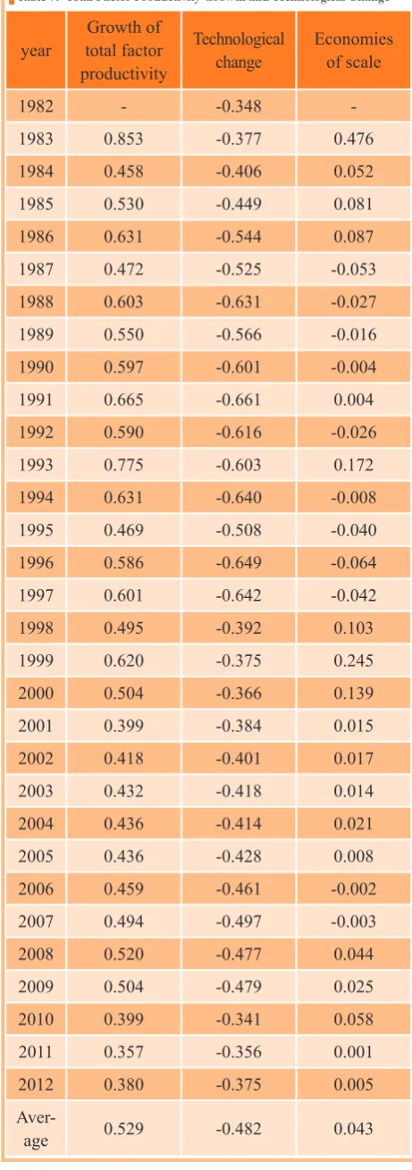
Accordingly, by estimating the cost function parameters and using equation (10), the growth of total factor productiv-ity was measured and divided into technological change and economies of scale. The results are shown in Table 7.

Through econometric approach, we also found that the annual average of total factor productivity was 0.529 per-cent over the study period. In general, this growth originated from two factors, the changes in technology and production unit size (production scale). In addition to the mentioned fac-tors, there were some other factors which affected productiv-ity of this sector like diversify oil and gas production and safety systems of production, transportation and consump-tion. There are other factors that had a negative impact on the efficiency of the petroleum refineries such as as aging refineries, depreciation facilities and the absence in the glob -al market. However, productivity growth in this sector was positive during the study period.

As Table 6 shows, improved total factor productivity was significantly affected by changes in technology. Due to the negative rate of technology change, it is characterized that the use of appropriate technology over time causes

de-Rate of technological change(percent) year

Rate of technological change(percent) year

-0.392 1998

-0.348 1982

-0.374 1999

-0.376 1983

-0.365 2000

-0.406 1984

-0.384 2001

-0.449 1985

-0.400 2002

-0.544 1986

-0.418 2003

-0.524 1987

-0.414 2004

-0.630 1988

-0.427 2005

-0.565 1989

-0.461 2006

-0.601 1990

-0.496 2007

-0.660 1991

-0.476 2008

-0.616 1992

-0.479 2009

-0.602 1993

-0.340 2010

-0.639 1994

-0.356 2011

-0.508 1995

-0.375 2012

-0.649 1996

--0.642 1997

Average of period = -0.482

Table 4: Rete of Technological Change

Return to Scale year

1.436 1998

2.239 1982

1.421 1999

2.128 1983

1.328 2000

2.415 1984

1.407 2001

2.063 1985

1.367 2002

1.624 1986

1.426 2003

1.244 1987

1.341 2004

1.201 1988

1.414 2005

1.324 1989

1.385 2006

1.193 1990

1.336 2007

1.672 1991

1.349 2008

1.725 1992

1.278 2009

1.563 1993

1.254 2010

1.162 1994

1.291 2011

1.627 1995

1.263 2012

1.583 1996

-1.427 1997

Average of the period = 1.267

(6)

Volume 1, Issue 1

November 2017

27

cline in the rate of change in the cost of production. Thus, the unit production is achievable by lower expending. On the other side, the increasing size of the production unit may lead to improved total factor productivity. Therefore, the re-sult of improvement in technology and production scale is observed through growth of total factor productivity in pe-troleum refineries industry.

7. Conclusions

Estimation of translog cost function and cost share equa-tions by SUR method in Iran’s petroleum refineries seems appropriate because many of coefficients are significant and R2 is relatively high. The sign of the rate of technological change show that over time, rate of change in the cost of production units was decreased. According to the results of our estimations, we realized that using new and advanced technology led to better cost change during the study period. Thus, it is expected to have more economic production in petroleum refineries through right technologies.

Moreover, our analyses, scale elasticity statistic indi-cates increasing return to scale in Iran’s petroleum refiner -ies i.e. production increases were more than the proportional change in all inputs, which in turn decreased per unit cost. And as a result Economies of scale was appeared in produc-tion process.

Over the study period, the results of our model on factor and scale biases in petroleum refineries also revealed that the factor bias and scale bias of labor and material were posi-tive while we observed high cost shares of these inputs out of total cost of inputs in production units. Consequently, we recommend that managers should be encouraged to enhance the productivity of the mentioned inputs in order to decrease production cost. Moreover, this type of technological change diminishes dependence on capital and energy and related costs.

Finally, based on the estimation results of the above mentioned models, we decomposed total factor productivity growth rate into the contributions of technological change

Scale Bias Factor Bias

Input

0.041 0.001

Labor

-0.397 -0.020

Capital

-0.004 -0.002

Energy

0.068 0.002

Material

Table 6: Factor and Scale Bias

Economies of scale Technological

change Growth of

total factor productivity year

--0.348

-1982

0.476 -0.377

0.853 1983

0.052 -0.406

0.458 1984

0.081 -0.449

0.530 1985

0.087 -0.544

0.631 1986

-0.053 -0.525

0.472 1987

-0.027 -0.631

0.603 1988

-0.016 -0.566

0.550 1989

-0.004 -0.601

0.597 1990

0.004 -0.661

0.665 1991

-0.026 -0.616

0.590 1992

0.172 -0.603

0.775 1993

-0.008 -0.640

0.631 1994

-0.040 -0.508

0.469 1995

-0.064 -0.649

0.586 1996

-0.042 -0.642

0.601 1997

0.103 -0.392

0.495 1998

0.245 -0.375

0.620 1999

0.139 -0.366

0.504 2000

0.015 -0.384

0.399 2001

0.017 -0.401

0.418 2002

0.014 -0.418

0.432 2003

0.021 -0.414

0.436 2004

0.008 -0.428

0.436 2005

-0.002 -0.461

0.459 2006

-0.003 -0.497

0.494 2007

0.044 -0.477

0.520 2008

0.025 -0.479

0.504 2009

0.058 -0.341

0.399 2010

0.001 -0.356

0.357 2011

0.005 -0.375

0.380 2012

0.043 -0.482

0.529

Aver-age

(7)

P

etroleum

B

usiness

R

eview

28

and economies of scale. The results showed that the share of technological change in the productivity growth is greater than that of scale economies which confirms the vital role of technological improvement in petroleum refining industry.

References

Atkinson, Anthony, and J. E. Stiglitz. (1969). A New View of Tecnological Change, Economic Journal, 79, 573-578. Baltagi, B. H. (2005). Econometrics Analysis of Panel Data.

John Wiley and Sons Ltd, 2005.

Baltagi, B. H. and J.M.Griffin. (1988). A General Index of Technical Change. Journal of Political Economy, 96:20_41. Bhattacharyya, S.C. (2011). Energy Economics, Concepts,

Issues, Markets and Governance. Springer-Verlag London. Binswanger, H. P. (1974). A Microeconomic Approach to

In-duced Innovation. Economic Journal, 84, 940- 958. Chambers, R. G. (1988). Applied Production Analysis: A

Dual Approach. Cambridge University Press.

Chen, K. and Edouard Wemy, (2015). Investment-specific technological changes: The source of long-run TFP fluctua -tions, European Economic Review, 80, 230- 252.

Datta, A., & Christoffersen, S. (2004). Production Costs, Scale Economies and Technical Change in U.S. Tex-tile and Apparel Industries. School of Business Administration,Philadelphia university.

Drandakis, E. M. and E. S. Phelps. (1966). A Model of In-duced Invention, Growth and Distribution, Economic Jour-nal. 76, 823-840.

Diewert, W. E. (1971). An Application of the Shephard Dual-ity Theorem: A Generalized Leontief Production Function. The Journal of Political Economy, 79(3), 481-507.

Grebel, Thomas, (2009). Technological change: A microeco-nomic approach to the creation of knowledge, Structural change and Economic Dynamics, 20, 301-312.

Gujarati, Damodar N. (2004). Basic Econometrics (4th ed.). McGraw-Hill.

Hart, Rob, (2013). Directed technological change and factor shares, Economics Letters, 119, 77-80.

Hayami, Y., & Godo, Y. (2005). Development Economics. Oxford University Press.

Iranian statistical center. Iranian report on industrial work-shops, various issues.

Intriligator, M. D. (1965). Embodied Technical Change and Productivity in the United States, 1929-1957. Review of Economics and Statistics, 47, 65-70.

Jorgenson, D. W. (1966). The Embodiment Hypothesis.

Jour-nal of Political Economy, 74, 1-17.

Kant, S., & Nautiyal, J. C. (1997). Production Structure, Factor Substitution, Technical Change, and Total Factor Productiv-ity. Canadian Journal of Forest Research, 27, 701-710. Krysiak, Frank C., (2011). Environmental regulation,

techno-logical diversity, and the dynamics of technotechno-logical change, Journal of Economic Dynamics and Control, 35, 528-544. Mattalia, Claudio, (2013). Embodied technological change

and technological revolution: Which sectors matter? Jour-nal of Macroeconomics, 37, 249-264.

McCarthy, M. D. (1965). Embodied and Disembodied Tech-nical Progress in the Constant Elasticity of Substitution Production Function. Review of Economics and Statistics, 47, 71-75.

Napasintuwong, O., & Emerson, R. D. (2002). Induced Inno-vations and Foreign Workers in U.S. Agriculture. Selected paper prepared for presentation of the American Agricul-tural Economics Association Annual Meeting, Califonia. Napasintuwong, O., & Emerson, R. D. (2003). Farm

Mecha-nization and the Farm Labor Market: A Socioeconomic Model of Induced Innovation. Selected paper prepared for presentation of the Southern Agricultural Economics Asso-ciation Annual Meeting. Mobile, A Labama.

Nordhaus, William D. (1969). An Economic Theory of Tech-nological Change, American Economic Review, 59, 18-28. Peretto, Pietro F., (1999). Industrial development, technologi-cal change, and long-run growth, Journal of Development Economics, 59, 389-417.

Rasmussen, S. (2000). Technological Change and Economies of Scale in Danish Agriculture. The Royal Eterinary and Agricultural University KVL, Copenhagen.

Romer, P. M. (1990). Endogenous Technological change. Journal of Politiocal Economy, 98, 71-102.

Roshef, Ariell, (2013). Is technological change biased to-wards the unskilled in services? An empirical investigation, Review of Economic Dynamics, 16, 312-331.

Salter Wilfred, E. J. (1960). Productivity and Technical Change, Cambridge University Press.

Schafer, Andreas, (2014). Technological change, population dynamics, and natural resource depletion, Mathematical Social Sciences, 71, 122-136.

Solow, R. M. (1957). Technical Change and the Aggregate Production Function. Review of Economics and Statistics, 39, 312-320.

Solow, R. M. (1962). Technical Progress, Capital Formation, and Economic Growth. American Economic Review, 52, 76-86. Stevenson, R. (1980). Measuring Technological Bias.