DEMOGRAPHIC RESEARCH
VOLUME 30, ARTICLE 57, PAGES 1571–1590
PUBLISHED 20 MAY 2014
http://www.demographic-research.org/Volumes/Vol30/57/ DOI: 10.4054/DemRes.2014.30.57
Research Article
The pace of aging: Intrinsic time scales in
demography
Tomasz F. Wrycza
Annette Baudisch
c
2014 Tomasz F. Wrycza & Annette Baudisch.
2 Properties and measures 1574
2.1 Properties of pace 1574
2.2 Measures of pace 1575
3 Pace-standardization 1578
3.1 Method 1578
3.2 Equivalence of pace measures with respect to standardizing 1580 3.3 Mortality: Standardized vs. unstandardized perspective 1581
4 Conclusion 1584
5 Acknowledgments 1584
References 1585
Appendices 1587
A Properties and measures 1587
The pace of aging: Intrinsic time scales in demography
Tomasz F. Wrycza1
Annette Baudisch2
Abstract
BACKGROUND
The pace of aging is a concept that captures the time-related aspect of aging. It formalizes the idea of a characteristic life span or intrinsic population time scale. In the rapidly developing field of comparative biodemography, measures that account for inter-species differences in life span are needed to compare how species age.
OBJECTIVE
We aim to provide a mathematical foundation for the concept of pace. We derive de-sired mathematical properties of pace measures and suggest candidates which satisfy these properties. Subsequently, we introduce the concept of pace-standardization, which reveals differences in demographic quantities that are not due to pace. Examples and consequences are discussed.
CONCLUSIONS
Mean life span (i.e., life expectancy from birth or from maturity) is intuitively appealing, theoretically justified, and the most appropriate measure of pace. Pace-standardization provides a serviceable method for comparative aging studies to explore differences in demographic patterns of aging across species, and it may considerably alter conclusions about the strength of aging.
1Max Planck Institute for Demographic Research, Rostock, Germany. E-Mail: [email protected].
1.
Introduction
Biodemography is a developing branch of demography that over recent decades has begun to study population dynamics and structure for non-human populations across the tree of life (Carey and Vaupel 2005; Vaupel 2010). With this development, methods to foster comparative research are increasingly sought after. For that purpose, Baudisch (2011) suggested a conceptual framework integrating approaches from life history biology that allows comparison of patterns of aging across species with vastly different life spans. The framework distinguishes between thepaceof life on one hand and the shapeof aging on the other. This distinction rests on the observation that different species live and die on different time scales. For example, the life course of a fruit fly is a matter of days, while the life course of humans is a matter of decades. The characteristic length of life for a species is taken as measure of the pace of life. Age and age-specific mortality are standardized by the pace of life to reveal the demographic aging pattern of a species, i.e. the shape of aging.
Pace-standardization of mortality disentangles the time scale (pace) and the change in the risk of death over the life course (shape). Thereby, the pace-shape distinction helps to unravel a problem that gerontologists face when they classify and rank species with respect to aging. Typically, gerontologists use the change in mortality to capture, on a demographic level, how organisms age. They compare rates of aging within and among species (Finch 1990). Rates, however, are given per unit time, say years, which leads to unfair comparisons when it comes to species that differ substantially in life span. Baudisch (2011) emphasizes that rates need to be pace-standardized to be meaningfully compared.
for different time scales has been suggested in the context of classic demography. Lee and Goldstein (2003) investigated rescaling the life cycle by means of a proportionality assumption, which under some circumstances is justified when comparing human popu-lations.
Demographers typically use standardization methods when it comes to comparing rates across populations that differ in population structure to avoid confounding compo-sitional effects (Preston, Heuveline, and Guillot 2001). By contrast, pace-standardization is not concerned with age-structure. In fact, differences in population composition will be the rule rather than the exception for most applications of pace-standardization. Pace-standardization solely aims to account for differences in time scales of life that differ across species. Differences in age structure and the spread in age at death are captured by the shape of aging. Shape measures whether mortality is increasing, constant, or decreas-ing over age, and whether these changes are more or less pronounced. Pace and shape are two complementary concepts that help characterize the aging pattern of a species in a comparative framework (Baudisch 2011).
Analysis of shape relies on the use of intrinsic time scales based on values of char-acteristic life span, i.e., on pace. A sound foundation for quantifying pace is therefore required. With the present study we thus wish to contribute a systematic investigation of alternative measures of pace. We provide a general approach to the pace-standardization of demographic functions that does not hinge (in the sense specified below) on the par-ticular choice of a measure. After deriving a list of desired mathematical properties of pace measures that enable us to evaluate the quality of each measure, we suggest different candidates. Subsequently, we formally explain the method of pace-standardization. It is a way of rescaling distributions according to their own specific pace value in order to make them comparablebeyondthe dimension of pace. We show that if two distributions are the same when standardized with respect to some pace measure, this will also be the case with respect to any other pace measure, as long as the pace measures satisfy a certain scaling property. Finally, we illustrate the significance of the procedure for compara-tive research on aging by showing the effect of pace-standardizing on several parametric mortality models (linear, Gompertz, Weibull). Results and implications are discussed.
of reproduction, though this is beyond the scope of the current work and needs to be thoroughly investigated in future research.
A notation alert: Demographic quantities are given in continuous formulation here and follow standard demographic notation. The survival function, which gives the probability of survival up to agex, is denoted asl(x). IfX is a positive random variable (life spans), the corresponding survival function is denoted as lX. The force of mortality or age-specific hazard is denoted asµwith
µ(x) =−l
0(x)
l(x).
The probability density function of death is
f(x) =−l0(x) =µ(x)l(x). (1)
Remaining life expectancy at agexis given by
e(x) = 1
l(x)
Z ∞
x
l(a)da.
A summary of notation and symbols is given in Appendix B.
2.
Properties and measures
What is the characteristic length of life? Previous approaches listed above apply a range of different measures commonly known to demographers, such as life expectancy, modal age at death, quantile measures of life span, or maximum life span. What measure should be preferred depends on the context. We will investigate which of the available measures is the most appropriate candidate to capture the pace of aging. As evaluation criteria we use a list of properties provided in the following, that, if fulfilled, facilitate pace-standardized analysis in demography.
2.1 Properties of pace
A pace measureMis a functionalM :l7→M(l)that assigns a non-negative real number
M(l)with dimension ’time’ to every survival function l. The following properties are desirable for pace measures.
P1: For allX it holds that
This scaling property ensures that if everybody’s life span changes by the factorr, then the value of pace changes by this factor as well (in more technical terms, it means that the functionalM is scale-invariant).
P2: For allXit holds that
M(lX+s) =M(lX) +s ∀s≥0. (3)
If everybody gains exactly s ≥ 0 years of life, the value of pace is the original pace value pluss. This would imply that no one dies before ages. While an age below which the probability of death is zero seems unrealistic, this property is conceptually helpful, because it follows thatP1andP2can be summarized by the simple property
M(ls+rX) =s+rM(lX) forr, s≥0, (4)
which means that ifX is transformed linearly,M(lX)is transformed accordingly. Expression (4) implies that a population in which everybody lives for exactlysyears has a pace value ofs, because
M(ls) =M(ls+0·s)
(4)
= s+ 0·M(ls) =s.
This appeals to intuition, as the concept of pace formalizes the idea of a characteristic life span.
P3:
µ1(x)≥µ2(x) ∀x ⇒ M(l1)≤M(l2). (5)
If two distributions are given so that the age-specific hazard of the first one is at all ages higher than or equal to the age-specific hazard of the second one, then the pace value of the first distribution is lower or equal to the pace value of the second one. This property reflects the fact that while pace captures the characteristic life span, its inverse is at the same time supposed to capture the level of the force of mortality. Thus, property P3
is important, because it emphasizes that the concept of pace is not only one of central tendency, but has an additional focus on the force of mortalityµ.
2.2 Measures of pace
1. An obvious first measure is the mean age at death (or life expectancy at age 0), which captures the average life span in the population:
e0= Z ∞
0
xf(x)dx=
Z ∞
0
l(x)dx=
Z ∞
0
1
µ(x)f(x)dx. (6)
This is a quantity widely used in demography, and it is a natural, straightforward answer to the question about a characteristic life span.
2. A generalization ofe0is given by the class of measures
Mg=
Z ∞
0
g(l(x))l(x)dx, (7)
wheregdenotes any absolutely continuous and monotonically non-decreasing func-tion
[0,1]→[0,1]
withg(1) = 1. Forg ≡ 1one getse0. Other choices ofg can also relateMgto known demographic quantities. For example, consider
g1(x) =x.
Then
Mg1 =
Z ∞
0
l2(x)dx=e0(1−G),
whereGdenotes the Gini coefficient, a measure of inter-individual inequality - see Hanada (1983) for a proof of the right hand side of the equality above and Shkol-nikov, Andreev, and Begun (2003) for an overview of the use ofGin demography.
3. Another class of pace measures{Mp|0< p <1}is defined in the following way: For every fixed0< p <1letMpbe the age (or rather the minimal age, in case it is not unique) at which the survival function reachesp:
Mp(l) = inf{x|l(x)≤p}.
M0.5is the median, the age up to which half of the cohort survives. Forpclose to
0, sayp = 0.01,Mpcorresponds to the age up to which only a small percentage of a given cohort survives (on average). Thus, in this caseMp provides a contin-uous approximation to a quantity frequently used in comparative aging research:
Pace measures e0, Mg andMp have several advantages and disadvantages from a demographic point of view.
Pace measuree0has the advantage of satisfying an additional, demographically
rele-vant property:
PA1: Ifl1, . . . , ln are survival functions andw1, . . . , wn > 0 are weights (so that
Pn
k=1wk= 1), then
l= n
X
k=1
wklk ⇒ M(l) = n
X
k=1
wkM(lk), (8)
which means that the pace value of the mixture distribution is the weighted mean of the pace values of the component distributions. For a proof see Appendix A. Depending on the application, PA1can be more or less desirable; in the context of frailty models for example, it may be important. e0is the only measure in the list above that satisfiesPA1;
in particular,PA1is not satisfied byMgifgis not constant.
One disadvantage of e0 (and more generally, of all pace measuresMg as defined above) is that the value of the integral can be infinite (for distributions where the age-specific hazard decreases strongly over age, or more generally heavy-tailed distributions), although this is unlikely to be found in demographically relevant life span distributions.
An advantage ofMg =R
∞
0 g(l(x))l(x)dxifgis not constant (i.e. ifMg 6=e0) can
be that - sincegis increasing - the later ages contribute less to the overall value of the measure. Thus the measure is more robust with respect to life spans that are very long, i.e. to outliers.
The quantile pace measuresMpdo not satisfyPA1. They do however satisfy a prop-erty which generalizes (4) to hold for a wider range of transformations instead of only linear ones:
PA2: If the random variableX has a continuous life span distribution and his a nonnegative, monotonically nondecreasing function (such as but not restricted to
-h(x) =s+rx), then
M(lh(X)) =h(M(lX)).
life spans not only contribute less to the value of the measure (which might be desired if the value is supposed to be less sensitive to outliers), they do not change its value at all.
As an observation, notice that the arithmetic average of any finite number of pace measures that satisfyP1andP2satisfiesP1andP2itself. For ifM1, . . . , Mnsatisfy (4), then for
M = 1
n
n
X
k=1
Mk
it holds that
M(ls+rX) = 1
n
n
X
k=1
Mk(ls+rX) = 1
n
n
X
k=1
(rMk(lX) +s) =rM(lX) +s.
IfM1, . . . , MnsatisfyP3in addition, then so doesM.
A classical measure of central tendency is the mode of a distribution, i.e. the age at which most deaths occur. However, while the mode can be useful in demographic context (see e.g. Canudas Romo 2008, 2010; Cheung and Robine 2007), it is not a good measure of pace. Even provided that it is unique (as is certainly the case for human populations if infant ages are omitted, but might not be the case for other species), the mode does not satisfy crucial propertyP3- see the appendix for a counterexample. Thus, this measure is not listed here.
3.
Pace-standardization
3.1 Method
Any pace measureM can be used to introduce a population-specific intrinsic time scale. Letxsdenote standardized age, which is a dimensionless number measuring age in units
of pace. It is therefore defined by dividing chronological agexby the value of pace:
xs= x
M. (9)
Standardized survival curves - functions of standardized age - can then be defined via
ls(xs) :=l(x) =l(M xs). (10)
used to derive an expression for the standardized hazard
µs(xs) =− 1
ls(xs) dls(xs)
dxs =−M
1
l(x)
dl(x)
dx =M µ(x) (=M µ(M x
s) ), (11)
which corresponds to a scaling along both the x- and the y-axis, with the scaling factors being M for the y-axis and M1 for the x-axis. These standardized functions are time-independent.
Note that the pace measuree0can be interpreted as the reciprocal of the population
average of the force of mortality in a twofold sense: Firstly, because
µ=
Z ∞
0
µ(x)c(x)dx=
Z ∞
0
µ(x)l(x)
e0
dx(1)= 1
e0
,
wherec(x) = l(ex)
0 denotes the age distribution in the stationary population. Secondly, because
1
e0
=
R∞ 0 f(x)dx R∞
0 1
µ(x)f(x)dx
and the right hand side of the equation is the weighted harmonic mean ofµ with the weights given by the pdff. Therefore, standardizing µwithM = e0 is conveniently
accomplished by dividing age by average life span and mortality by average mortality,
xs= x
e0
, µs(xs) = µ(x)
µ , (12)
which appeals to intuition.
Within the standardized framework, all mortality patterns have the same pace value (namely1), because
lsX(xs) =lX(M(lX)xs) =l X M(lX)(x
s) ∀xs
P1
=⇒
M(lsX) =M(l 1
M(lX)X) =
1
M(lX)
·M(lX) = 1.
This property justifies the name ’standardization’.
As each demographic function can be expressed in terms of survivall, standardized in (10), one can derive standardized expressions for these functions as well:
fs(xs) =M f(x), es(xs) =e(x)
3.2 Equivalence of pace measures with respect to standardizing
Assume two pace measuresM1andM2, both satisfyingP1. Denote standardization with
respect toM1andM2with the upper indices s1and s2respectively. Assume further two
positive random variables with survival functionslX1andlX2so that
ls1 X1=l
s1
X2. (14)
Then it also holds that
ls2 X1=l
s2
X2.
This means that if two distributions of ages at death give the same standardized distribu-tion with respect to measureM1, they also give the same standardized distribution with
respect to measureM2.
Proof:From (14) it follows that
lX1(zM1(lX1)) =lX2(zM1(lX2)) ∀z,
or, withy=zM1(lX1):
lX1(y) =lX2
yM1(lX2)
M1(lX1)
∀y, (15)
which implies
lX1 =lM1 (lX1)
M1 (lX2)
X2
.
BecauseM2satisfiesP1, this implies
M2(lX1) =
M1(lX1)
M1(lX2)
M2(lX2),
so that
M1(lX2)
M1(lX1)
= M2(lX2)
M2(lX1)
.
Inserting this into (15) gives
lX1(y) =lX2
yM2(lX2)
M2(lX1)
∀y,
and thus withw= M y 2(lX1)
which implies
ls2 X1 =l
s2
X2. Q.E.D.
Pace-standardization can be seen as providing an equivalence relation on life span distributions: Two distributions are equivalent if they give the same standardized distribu-tion. The result above states that if two pace measures satisfy propertyP1, they provide the same partition into equivalence classes, regardless of how their actual values might differ.
3.3 Mortality: Standardized vs. unstandardized perspective
The age-specific force of mortality (or hazard of death) is an important quantity for biode-mographic research on aging patterns of different species, and standardized depictions of mortality and other vital rates have recently been used to reveal the diversity of patterns across species (Jones et al. 2014). It is therefore instructive to see how pace-standardizing simple hazard functions can give results that drastically differ from the unstandardized perspective. For this subsection the pace measure isM =e0.
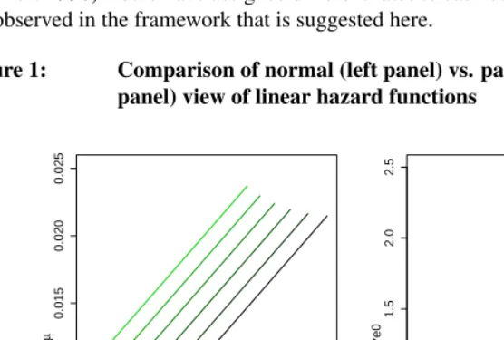
First, assume a linearly increasing force of mortality
µ(x) =bx+c
with fixed b = 0.0001, and letc vary between0.001 and0.01. Figure 1 depicts the resulting hazard functions with the ’normal’ perspective (i.e.µ(x)over chronological age
x) on the left and the pace-standardized perspective (i.e. µs(xs)overxs = x
e0) on the right. Lighter color indicates higher values ofc.
Comparing these two alternative views reveals a striking difference: While in the normal view all the curves have the same slope, so that a common interpretation would conclude that all the populations in question experience the same strength of aging, the pace-standardized view reveals that the highercis, the lower the slope of the curve turns out to be, i.e. the less aging the population in question experiences.
As another example, assume Gompertz mortality defined as
µ(x) =aebx
with fixed b = 0.1, and letavary between0.00001 and0.0002. Figure 2 depicts the resulting hazard functions, again both from normal and pace-standardized perspective. Lighter color corresponds to higher values ofa(hazard is presented on a log-scale).
slope - and thus, the common interpretation ofb as the ’rate of aging’ would conclude that all the populations in question experience the same strength of aging. But the pace-standardized view reveals that the higherais, the lower the slope of log-mortality turns out to be, i.e., that the pace-standardized rate of agingbe0 implies less aging for higher
values ofa.
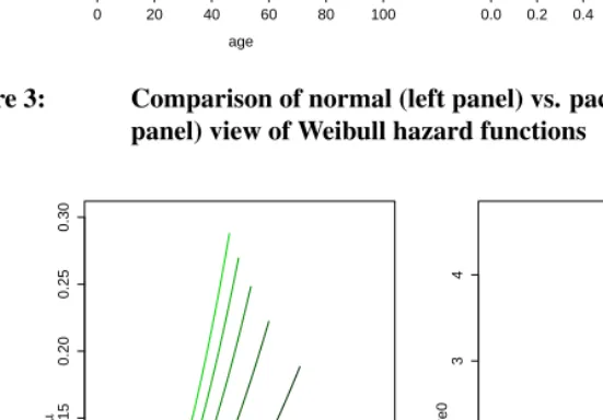
As a last example, assume Weibull mortality defined as
µ(x) =αxβ
with fixedβ = 2, and letαvary between0.00005and0.0005. Figure 3 depicts the re-sulting hazard functions, again both from both normal and pace-standardized perspective. Lighter color indicates higher values ofα.
In this case, it turns out that all the pace-standardized schedules fall on the same line, i.e., that parameterαdoes not influence the pace-standardized hazard functionat all(this can also be shown analytically, see Appendix A). Parameterβ is all that matters for the shape of the standardized curve. While Ricklefs’ “rate of aging“ defined asω =αβ1+1 (Ricklefs 1998) would have assigned different rates to each curve, no differences in shape are observed in the framework that is suggested here.
Figure 1: Comparison of normal (left panel) vs. pace-standardized (right panel) view of linear hazard functions
0 50 100 150 200
0.000
0.005
0.010
0.015
0.020
0.025
age
µ
0.0 0.5 1.0 1.5 2.0
0.5
1.0
1.5
2.0
2.5
age/e0
µ
Figure 2: Comparison of normal (left panel) vs. pace-standardized (right panel) view of Gompertz hazard functions
0 20 40 60 80 100
−10
−8
−6
−4
−2
age
log
(
µ
)
0.0 0.2 0.4 0.6 0.8 1.0 1.2
−6
−4
−2
0
2
age/e0
log
(
µ
*e0
)
Figure 3: Comparison of normal (left panel) vs. pace-standardized (right panel) view of Weibull hazard functions
0 10 20 30 40 50
0.00
0.05
0.10
0.15
0.20
0.25
0.30
age
µ
0.0 0.5 1.0 1.5
0
1
2
3
4
age/e0
µ
4.
Conclusion
Comparative aging research that aims to find and measure differences in demographic aging patterns across species is an exciting and rapidly developing field (Baudisch and Vaupel 2012; Jones et al. 2014; Baudisch et al. 2013), and it crucially hinges on service-able methods.
To facilitate meaningful comparison between different species, with this paper we provide a systematic discussion of 1) how the time aspect of aging can be measured, 2) how pace measures can be used as an intrinsic time scale to create pace-standardized demographic functions, and of 3) why this procedure does not hinge on the particular choice of a measure (in the sense specified in 3.2). We conclude that of all the candidates for pace measures discussed here,e0is the one to be preferred (if its value is available),
because it additionally satisfies property PA1 concerning mixture distributions, which is demographically relevant. All measures of life span commonly used in demographic applications have been discussed in the present analysis, although further candidates may exist.
The examples in 3.3 show that the difference between unstandardized and standard-ized perspectives can be immense if one compares mortality curves. Conclusions about the strength of aging may change and even reverse when switching perspectives. There-fore, the methods discussed here may prove useful to researchers who investigate differ-ences in demographic aging patterns between different populations/species - in particular if the populations in question differ significantly with respect to how long they live, i.e., in their pace values.
5.
Acknowledgments
References
Baudisch, A. (2011). The pace and shape of ageing. Methods in Ecology and Evolution 2(4): 375–382.doi:10.1111/j.2041-210X.2010.00087.x.
Baudisch, A., Salguero-Gomez, R., Jones, O., Wrycza, T., Mbeau-Ache, C., Franco, M., and Colchero, F. (2013). The pace and shape of senescence in angiosperms.Journal of Ecology101(3): 596–606.doi:10.1111/1365-2745.12084.
Baudisch, A. and Vaupel, J. (2012). Getting to the root of aging. Science338(6107): 618–619.doi:10.1126/science.1226467.
Canudas Romo, V. (2008). The modal age at death and the shifting mortality hypothesis. Demographic Research19: 1179–204. doi:10.4054/DemRes.2008.19.30.
Canudas Romo, V. (2010). Three measures of longevity: time trends and record values. Demography47(2): 299–312. doi:10.1353/dem.0.0098.
Carey, J. and Vaupel, J. (2005). Biodemography. In: Poston, D. and Micklin, M. (eds.). Handbook of Population. New York:Kluwer Academic/Plenum: 625–658.
Charlesworth, B. (1994). Evolution in age-structured populations. New Jersey: Univer-sity of Cambridge Press.doi:10.1017/CBO9780511525711.
Cheung, S. and Robine, J. (2007). Increase in common longevity and the com-pression of mortality: The case of japan. Population Studies 61(1): 85–97.
doi:10.1080/00324720601103833.
Coale, A. (1972).The growth and structure of human populations: a mathematical inves-tigation. Princeton: Princeton University Press.
Deevey, E. (1947). Life tables for natural populations of animals. The Quarterly Review of Biology22(4): 283–314. doi:10.1086/395888.
Deevey, E. (1950). The probability of death. Scientific American 182(4): 58–60.
doi:10.1038/scientificamerican0450-58.
Eakin, T. (1994). Intrinsic time scaling in survival analysis: applications to biological populations. Bulletin of Mathematical Biology 56(6): 1121–1141.
doi:10.1007/BF02460289.
Eakin, T. and Witten, M. (1995). A gerontological distance metric for analysis of survival dynamics.Mechanisms of Ageing and Development78(2): 85–101. doi:10.1016/0047-6374(94)01508-J.
Press.
Hanada, K. (1983). A formula of Gini’s concentration ratio and its application to life tables.Journal of Japan Statistical Society13(2): 95–98.
Jones, O., Scheuerlein, A., Salguero-Gomez, R., Camarda, C., Schaible, R., Casper, B., Dahlgren, J., Ehrlen, J., Garcia, M., Menges, E., Quintana-Ascencio, P., Caswell, H., Baudisch, A., and Vaupel, J. (2014). Varieties of ageing across the tree of life.Nature 505(7482): 169–173.doi:10.1038/nature12789.
Lee, R. and Goldstein, J. (2003). Rescaling the Life Cycle: Longevity and Proportionality. Population and Development Review29: 183–207.
Lynch, H., Zeigler, S., Wells, L., Ballou, J., and Fagan, W. (2010). Survivorship patterns in captive mammalian populations: implications for estimating populations growth rates. Ecological Applications20(8): 2334–2345. doi:10.1890/09-1276.1.
Pearl, R. (1928).The Rate of Living. New York: Alfred A. Knopf.
Pearl, R. and Miner, J. (1935). Experimental studies on the duration of life. XIV: The comparative mortality of certain lower organisms. The Quarterly Review of Biology 10(1): 60–79.doi:10.1086/394476.
Preston, S., Heuveline, P., and Guillot, M. (2001).Demography: Measuring and Model-ing Population Processes. Oxford: Blackwell.
Ricklefs, R. (1998). Evolutionary theories of aging: confirmation of a fundamental pre-diction, with implications for the genetic basis and evolution of life span.The American Naturalist152(1): 24–44.doi:10.1086/286147.
Shkolnikov, V., Andreev, E., and Begun, A. (2003). Gini coefficient as a life table func-tion: computation from discrete data, decomposition of differences and empirical ex-amples.Demographic Research8(11): 305–358. doi:10.4054/DemRes.2003.8.11.
Vaupel, J. (2010). Biodemography of human ageing. Nature 464(7288): 536–542.
doi:10.1038/nature08984.
Weon, B. and Je, J. (2011). Plasticity and rectangularity in survival curves. Scientific Reports1(104).doi:10.1038/srep00104.
Appendix
A
Properties and measures
Note that
ls+rX(x) =
(
1 x≤s, lX(x−rs) x > s.
(16)
This relationship is needed for the following proofs.
Proof that Mg satisfies (4) for any absolutely continuous and monotonically non-decreasing
g: [0,1]→[0,1]
withg(1) = 1:
Mg(ls+rX) =
Z ∞
0
g(ls+rX(x))ls+rX(x)dx=
(16)
=
Z s
0
g(1)dx+
Z ∞
s
g
lX
x−s r
lX
x−s r
dx=
z=x−rs
= s+r
Z ∞
0
g(lX(z))lX(z)dz=s+rMg(lX).
Q.E.D.
Proof that for eachp,Mpsatisfies (4): Let0< p <1be fixed. For everyxwith
lX(x)≤p
it holds that
ls+rX(s+rx)
(16)
= lX(x)≤p.
Conversely, anyywithls+rX(y)≤p <1has to be> sand forx= y−rsit holds that
lX(x) =ls+rX(y)≤p.
It follows that
{y|ls+rX(y)≤p}={s+rx|lX(x)≤p},
Proof that Mg satisfies P3for any absolutely continuous and monotonically non-decreasing
g: [0,1]→[0,1]
withg(1) = 1: Because
µ1(x)≥µ2(x) ∀x ⇒ l1(x)≤l2(x) ∀x,
and, becausegis monotonically non-decreasing, also
g(l1(x))≤g(l2(x)) ∀x,
it follows that
Mg(l1) = Z ∞
0
g(l1(x))l1(x)dx≤ Z ∞
0
g(l2(x))l2(x)dx=Mg(l2).
Q.E.D.
For the quantile measuresMp,P3follows directly from the fact that
µ1(x)≥µ2(x) ∀x ⇒ l1(x)≤l2(x) ∀x.
Proof that the mode of a distribution does not satisfyP3:
Assume linearly increasing mortalityµ(x) =bx+c. By settingf0(x) = l(x)(µ0(x)−
µ2(x)) = 0in order to find the maximum off, one finds that the mode is √1
b − c b. If
c >0is kept fixed, this value is0whenb=c2, then increases withbas long asb≤4c2, and afterwards decreases asbincreases. For example, ifc= 0.01, forb1= 3c2= 0.0003
the mode is≈24.4, while forb2 = 4c2 = 0.0004, the mode is25and thus bigger than
forb1. Butb1 ≤b2means thatµ1(x)≤µ2(x)∀x, which according toP3would imply
M(l1)≥M(l2), which is not the case. Thus the mode does not in general satisfyP3.
Q.E.D.
Proof that of all the measures presented, onlye0satisfiesPA1:
For the measuresMgassume
l1(x) = (
1 0≤x≤2,
0 x >2,
l2(x) = (
1 0≤x≤1,
Then for any given0< w <1considerlw=wl1+ (1−w)l2, so that
lw(x) =
1 0≤x≤1,
w 1< x≤2,
0 x >2.
SinceMg(l1) = 2andMg(l2) = 1, it holds that
wMg(l1) + (1−w)Mg(l2) = 1 +w.
On the other hand,
Mg(lw) =
Z 1
0
g(1)dx+
Z 2
1
g(w)w dx= 1 +wg(w),
so that ifPA1holds,g(w) = 1. But this is true forany0 < w <1, so thatg ≡1is the only function for whichMggives a measure satisfyingPA1.
For the quantile measuresMpassumel1(x) =e−x,l2(x) =e−2x,w1 =w2 = 0.5
and a 0 < p < 1 fixed. Then Mp(l1) = −log(p) andMp(l2) = −12log(p). For
l(x) = 0.5(l1(x) +l2(x))it holds that
l
1
2(Mp(l1) +Mp(l2))
=l
−3 4log(p)
= 1 2(p
3
4 +p32)6=p,
so that
Mp(l)6=w1Mp(l1) +w2Mp(l2).
Q.E.D.
Proof that if a measureM satisfiesPA2, then there exists a0< p <1withM =Mp (withMpreferring to the quantile measures as defined in subsection 2.2):
The proof relies on the probability integral transform. IfFY is the cumulative distribu-tion funcdistribu-tion of the random life span variableY, then the random variableZ=FY(Y) = 1−lY(Y)is uniformly distributed on[0,1], and the cumulative distribution function of
FY−1(Z)isFY.FY−1(u) = inf{y|FY(y)≥u}is a monotone non-decreasing function, so thatPA2withh=FY−1andX =Zgives
M(lY) =FY−1(M(lZ)),
and thus
wherep=M(lZ)is a fixed value not depending onY, so thatM(lY) =Mp(lY). Q.E.D.
Proof that for the Weibull mortalityµ(x) =αxβ, parameterαdoes not influence the standardized distribution, i.e., thatµ1(x) =α1xβ,µ2(x) =α2xβimpliesµs1=µs2:
We choosee0 as the pace measure (as shown in 3.2, the particular choice of a pace
measure does not matter). Ifω=αβ1+1, then
µ(x) =ω(ωx)βandl(x) =e−β+11 (ωx)
β+1
.
This implies
e0= Z ∞
0
l(x)dxz==ωx 1
ω
Z ∞
0
e−zβ
+1
β+1dz=C(β)
ω
with a functionC(β)depending only onβ. This means
ls(xs) =l(xse0) =e−
1
β+1(C(β)x
s)β+1
,
which does not depend onα. Thusµsalso does not depend onα.
Q.E.D.
B
Overview of notation
Symbol Meaning
x age
ω maximum life span
X, Y random variables (of age at death) Mg Pace Measure (specified by subscript) l(x) Survival function
lX(x) Survival function corresponding to rand. var.X µ(x) Force of mortality, age-specific hazard f(x) Probability density function of age at death e(x) Remaining life expectancy (as function ofx) e0 Life expectancy at age zero
xs, ls, µs, fses Quantities standardized