Analytical approximate solution of leptospirosis epidemic model with
standard incidence rate
Rukhsar Ikram
Department of Mathematics and Statistics, University of Swat, Khyber Pakhtunkhwa, Pakistan. E-mail: ikramrukhsar@gmail.com
Amir Khan∗
Department of Mathematics and Statistics, University of Swat, Khyber Pakhtunkhwa, Pakistan. E-mail: amir.maths@gmail.com
Asaf Khan
Department of Mathematics, University of Malakand, Chakdara, Dir(Lower), Khyber Pakhtunkhwa, Pakistan. E-mail: asafkhan319@ymail.com
Tahir Khan
Department of Mathematics, University of Malakand, Chakdara, Dir(Lower), Khyber Pakhtunkhwa, Pakistan. E-mail: tahirmaths200014@gmail.com
Gul Zaman
Department of Mathematics, University of Malakand, Chakdara, Dir(Lower), Khyber Pakhtunkhwa, Pakistan. E-mail: talash74@yahoo.com
Abstract In this paper, we consider a mathematical model of leptospirosis disease which is an infectious disease. The model we are considering is a system of nonlinear ordinary differential equations and it is difficult to find exact solution. He’s homotopy per-turbation method is employed to compute an approximation to the solution of the system of nonlinear ordinary differential equations governing on the problem. The findings obtained by HPM are compared with nonstandard finite difference (NSFD) and Runge-Kutta fourth order (RK4) methods. Some plots are presented to show the reliability and simplicity of the method.
Keywords. Leptospirosis, Homotopy perturbation method, Epidemic model, Numerical simulations.
2010 Mathematics Subject Classification. 92D25, 49J15, 93D20.
Received: 21 January 2018 ; Accepted: 18 November 2018.
∗Corresponding author.
1. Introduction
Mathematical modeling has become an important tool in analyzing the spread and control of infectious diseases [12,13]. These models help us to understand different factors like the transmission and recovery rates and predict how the diseases will spread over a period of time. In the past decades, leptospirosis infection has arisen as a globally important contagious disease. This type of disease occurred in the urban regions of developed and industrialized countries and in the rural areas as well across the globe. Individual belonging to very crowded area especially in a city and not using clean water are usually infected with this disease. Sewer cleaners, rice planters, agriculture labor and workers that cleans the canals can easily contact with this infection. There are two main reasons which are responsible for significant mortality rate due to leptospirosis: delays in diagnosis of the disease and pathogenicity of some leptospiral rinsing.
Numerous models have been investigated which represents the dynamics of both human and vector populations of SIR type as described in [3–5]. In order to study the dynamical aspects of leptospirosis disease, Pongsuumpun et al. in [14] proposed a very simple mathematical model. In their work, they studied the dynamics of both rats and human populations as the time evolve. The human population was further stratified into two groups; adults and juveniles. A deterministic model for the dynamics of leptospirosis disease was proposed by Triampo et al. [17]. They consider a case study of leptospirosis in Thailand and present some numerical results. Zaman [18] considered the real data of [17] and studied the transmission dynamics and the role of optimal control theory of leptospirosis.
Since, most of the mathematical models raised from biological problems are non-linear by nature and it is difficult to find the analytical solution of such problems. Therefore, it is a great challenge for mathematicians and researchers to find such nu-merical and perturbation methods which give the best approximation to the solution of such nonlinear problems. Convergence and accuracy are the key concepts while developing and implementing a numerical scheme otherwise results will be inappro-priate. As far as the analytical perturbation methods are concerned, a parameter (negligibly small) needs to be exerted in the equation. Exertion and production of such parameter is a difficult task in these methods. Recent research provided powerful methods like artificial parameter method in which this small parameter is absent.
This work is an extension of [8–11] by considering HPM applied to leptospirosis epidemic model. We will compare the results obtained by HPM with Runge-Kutta fourth order (RK4) method. The motivations of this method are: the method can be applied both to linear and nonlinear problems with no discretization or linearization. Numerous problems of nonlinear nature can be solved accurately and effectively using HPM because of its rapid convergence [1,2,6,15,16].
The rest of manuscript is as follow. In section 2 we included the basic concept of HPM. The model is formulated and solved by HPM in section 3. Sample numerical result and discussion is given in section 4. Conclusion is presented at the end of the paper.
2. Analysis of Homotopy Perturbation Method (HPM)
To illustrate the basic idea of HPM, consider the general nonlinear differential equation
A(µ)−f(r) = 0, r∈Ω, (2.1)
with the boundary condition,
β(µ,δµ
δn) = 0, r∈Γ, (2.2)
where A is a general differential operator, β is a boundary operator, f(r) a known analytic function, Γ is the boundary of the domain Ω. The operatorAis divided into linear partLand nonlinear partN. Therefore, equation (2.1) can be written as,
L(u) +N(u)−f(r) = 0. (2.3)
By using the homotopy technique, one can construct a homotopy
υ(r, p) : Ω×[0,1]−→R (2.4)
which satisfies
H(υ, p) = (1−p)[L(υ)−L(µ0)] +p[A(υ)−f(r)] = 0, (2.5)
or
H(υ, p) =L(υ)−L(µ0) +pL(υ0) +p[N(υ)−f(r)] = 0, (2.6)
where p ∈ [0,1] is an embedding parameter and µ0 is the initial approximation of
given equation that satisfies the boundary conditions. Clearly, we have
H(υ,0) =L(υ)−L(µ0) = 0, (2.7)
H(υ,1) =A(υ)−f(r) = 0. (2.8)
The changing process ofpfrom zero to one is just that ofυ(r, p) changing fromµ0(r)
toµ(r). This is called deformation, and alsoL(υ)−L(µ0) andA(υ)−f(r) are called
homotopic in topology. If the embedding parameterp(0 ≤p≤1) is considered as a small parameter, applying the classical perturbation technique, we can naturally assume that the solution of the equation can be given as a power series inp,
Settingp= 1 results in the approximate solution as
υ= lim
p→1υ=υ0+υ1+υ2+υ3+... (2.10)
3. Mathematical formulation
In this section, we extend the model presented in [6] by taking into account the interaction of susceptible human with infected vector and disease related death rate in both infected human and vectors. To understand the basic properties of the epidemic model, we first formulate the model in detail and define the parameter involve in the model. To this end, we assume thatSh(t) represents number of susceptible human
at time t; Ih(t) represents number of human in the population, which is infected
from the leptospirosis disease at time t; Rh(t) represents number of human in the
population which is recovered at time t; we denote the total population size byNh,
with Nh(t) = Sh(t) +Ih(t) +Rh(t). For vector population, letSv(t) is susceptible
vector and Iv(t) is infectious vector at time t. The total population size of vector
population is denoted byNv withNv(t) =Sv(t) +Iv(t).
dSh
dt = b1Nh−µhSh− β2ShIv
Nv −
β1ShIh
Nh +λhRh,
dIh
dt =
β2ShIv
Nv +
β1ShIh
Nh −µhIh−δhIh−γhIh,
dRh
dt = γhIh−µhRh−λhRh,
dSv
dt = b2Nv−γvSv− β3SvIh
Nh ,
dIv
dt =
β3SvIh
Nh −γvIv−δvIv,
(3.1)
with initial conditions
Sh(0)≥0, Ih(0)≥0, Rh(0)≥0, Sv(0)≥0, Iv(0)≥0. (3.2)
Here b1 is the recruitment rate of human population, susceptible human can be
in-fected by two ways of transmission,β1which represents the direct transmission from
infected human and β2 is the rate of transmission from infected vector. µh is the
natural mortality rate of human,λh is the recovery rate of human. In this work, we
assumed that disease may be fatal to some infectious host, soδhrepresents the disease
related death rate of infected individuals. The rate of recovery from the infection is shown byγh. b2 is the recruitment rate of vector population. γv is the natural
mor-tality rate of vector population. The infectious vector die due to disease at a rate of
Now, we apply the homotopy perturbation technique to our model (3.1). To do this, first we define the operatorL= dtd. The homotopy of above system is
LSh(t)−LSh0(t) = p
[
b1Nh−µhSh−β2NShvIv −β1NShhIh +λhRh−LSh0(t)
]
,
LIh(t)−LIh0(t) = p
[
β2ShIv
Nv +
β1ShIh
Nh −µhIh−δhIh−γhIh−LIh0(t) ]
,
LRh(t)−LRh0(t) = p
[
γhIh−µhRh−λhRh−LRh0(t)
]
,
LSv(t)−LSv0(t) = p
[
b2Nv−γvSv−β3NSvIh
h −LSv0(t) ]
,
LIv(t)−LIv0(t) = p
[
β3SvIh
Nh −γvIv−δvIv−LIv0(t) ]
.
(3.3)
We assume that the solution of the system (3.3) is in the form,
Sh(t)=Sh0+pSh1+p2Sh2+...
Ih(t)=Ih0+pIh1+p2Ih2+...
Rh(t)=Rh0+pRh1+p2Rh2+...
Sv(t)=Sv0+pSv1+p2Sv2+...
Iv(t)=Iv0+pIv1+p2Iv2+...
(3.4)
Considering (3.4) in (3.3), and comparing the same coefficient, we obtain,
LSh1 = b1Nh−µhSh0−
β2Sh0Iv0
Nv −
β1Sh0Ih0
Nh +λhRh0−LSh0,
LIh1 =
β2Sh0Iv0
Nv +
β1Sh0Ih0
Nh −µhIh0−δhIh0−γhIh0−LIh0,
LRh1 = γhIh0−µhRh0−λhRh0−LRh0,
LSv1 = b2Nv−γvSv0−
β3Sv0Ih0
Nh −LSv0,
LIv1 =
β3Sv0Ih0
Nh −γvIvo−δvIv0−LIv0,
and
LSh2 = µhSh1−β2SNh1vIv0 −β1SNh0Ih1
h −
β1Sh1Ih0
Nh −
β2Sh0Iv1
Nv ,
LIh2 = β2SNh1vIv0+
β2Sh0Iv1
Nv +
β1Sh0Ih1
Nh +
β1Sh1Ih0
Nh −µhIh1−δhIh1−γhIh1,
LRh2 = γhIh1−µhRh1−λhRh1,
LSv2 = −γvSv1−β3SNv0Ih1
h −
β3Sv1Ih0
Nh ,
LIv2 = β3SNv1hIh0+β3SNv0hIh1 −γvIv1−δvIv1.
(3.6)
In order to obtain the solution of the zeroth order problem, we consider the fol-lowing cases.
Zeroth Order Problem or P0
Sh0= 130, Ih0= 90, Rh0= 70, Sv0= 150, Iv0= 60, Nh= 290, Nv= 210.
(3.7)
First Order Problem or P1
Sh1 = (b1Nh−µhSh0−
β2Sh0Iv0
Nv −
β1Sh0Ih0
Nh +λhRh0)t,
Ih1 = (
β2Sh0Iv0
Nv +
β1Sh0Ih0
Nh −µhIh0−δhIh0−γhIh0)t,
Rh1 = (γhIh0−µhRh0−λhRh0)t,
Sv1 = (b2Nv−γvSv0−
β3Sv0Ih0
Nh )t,
Iv1 = (
β3Sv0Ih0
Nh −γvIvo−δvIv0)t.
(3.8)
Second Order Problem or P2
Sh2=
[
µh(b1Nh−µhSh0−
β2Sh0Iv0
Nv −
β1Sh0Ih0
Nh
+λhRh0)−
β2
Nv
(b1Nh−µhSh0
−β2Sh0Iv0
Nv
−β1Sh0Ih0
Nh
+λhRh0)Iv0−
β1Sh0
Nv
(β2Sh0Iv0
Nv
+β1Sh0Ih0
Nh
−µhIh0−δhIh0−γhIh0)−
β1Ih0
Nh
(b1Nh−µhSh0−
β2Sh0Iv0
Nv
−β1Sh0Ih0
Nh
+λhRh0)
−β2Sh0
Nv
(β3Sv0Ih0
Nh −
γvIvo−δvIv0)
]
Ih2=
[
β2
Nv
(b1Nh−µhSh0−
β2Sh0Iv0
Nv −
β1Sh0Ih0
Nh
+λhRh0)Iv0+
β1Sh0
Nv
(β2Sh0Iv0
Nv
+β1Sh0Ih0
Nh
−µhIh0−δhIh0−γhIh0)+
β1Ih0
Nh
(b1Nh−µhSh0−
β2Sh0Iv0
Nv
−β1Sh0Ih0
Nh
+λhRh0) +
β2Sh0
Nv
(β3Sv0Ih0
Nh
−γvIvo−δvIv0) + (µh+δh+γh)
(β2Sh0Iv0
Nv
+β1Sh0Ih0
Nh
−µhIh0−δhIh0−γhIh0)
]
t2/2, (3.10)
Rh2=
[
γh(
β2Sh0Iv0
Nv
+β1Sh0Ih0
Nh
−µhIh0−δhIh0−γhIh0)
−(µh+λh)(γhIh0−µhRh0−λhRh0)
]
t2/2, (3.11)
Sv2=
[
−γv(b2Nv−γvSv0−
β3Sv0Ih0
Nh
)−β3Sv0
Nh
(β2Sh0Iv0
Nv
+β1Sh0Ih0
Nh
−µhIh0−δhIh0−γhIh0)−
β3Ih0
Nh
(b2Nv−γvSv0−
β3Sv0Ih0
Nh
) ]
t2/2, (3.12)
Iv2=
[
β3Sv0
Nh
(β2Sh0Iv0
Nv
+β1Sh0Ih0
Nh −
µhIh0−δhIh0−γhIh0) +
β3Ih0
Nh
(b2Nv
−γvSv0−
β3Sv0Ih0
Nh
)−(γv+δv)(
β3Sv0Ih0
Nh
−γvIvo−δvIv0)
]
t2/2. (3.13)
To find the solution we considerp= 1 in the system (3.4), we get
Sh(t)=Sh0+Sh1+Sh2+...
Ih(t)=Ih0+Ih1+ 2Ih2+...
Rh(t)=Rh0+Rh1+ 2Rh2+...
Sv(t)=SV0+SV1+ 2SV2+...
Iv(t)=IV0+IV1+ 2IV2+...
Sh(t) =Sh0+ (b1Nh−µhSh0−
β2Sh0Iv0
Nv −
β1Sh0Ih0
Nh
+λhRh0)t
+ [
µh(b1Nh−µhSh0−
β2Sh0Iv0
Nv −
β1Sh0Ih0
Nh
+λhRh0)
− β2
Nv
(b1Nh−µhSh0−
β2Sh0Iv0
Nv −
β1Sh0Ih0
Nh
+λhRh0)Iv0−
β1Sh0
Nv
(β2Sh0Iv0
Nv
+β1Sh0Ih0
Nh −
µhIh0−δhIh0−γhIh0)−
β1Ih0
Nh
(b1Nh−µhSh0−
β2Sh0Iv0
Nv
−β1Sh0Ih0
Nh
+λhRh0)−
β2Sh0
Nv
(β3Sv0Ih0
Nh −
γvIvo−δvIv0)
]
t2/2, (3.15)
Ih(t) =Ih0+ (
β2Sh0Iv0
Nv
+β1Sh0Ih0
Nh
−µhIh0−δhIh0−γhIh0)t
+ [
β2
Nv
(b1Nh−µhSh0−
β2Sh0Iv0
Nv
−β1Sh0Ih0
Nh
+λhRh0)Iv0+
β1Sh0
Nv
(β2Sh0Iv0
Nv
+β1Sh0Ih0
Nh −
µhIh0−δhIh0−γhIh0) +
β1Ih0
Nh
(b1Nh−µhSh0−
β2Sh0Iv0
Nv
−β1Sh0Ih0
Nh
+λhRh0) +
β2Sh0
Nv
(β3Sv0Ih0
Nh −
γvIvo−δvIv0) + (µh+δh+γh)
(β2Sh0Iv0
Nv
+β1Sh0Ih0
Nh −
µhIh0−δhIh0−γhIh0)
]
t2/2, (3.16)
Rh(t) =Rh0+ (γhIh0−µhRh0−λhRh0)t+
[
γh(
β2Sh0Iv0
Nv
+β1Sh0Ih0
Nh
−µhIh0−δhIh0−γhIh0)−(µh+λh)(γhIh0−µhRh0−λhRh0)
]
t2/2,
(3.17)
Sv(t) =Sv0+ (b2Nv−γvSv0−
β3Sv0Ih0
Nh
)t+ [
−γv(b2Nv−γvSv0−
β3Sv0Ih0
Nh
)−β3Sv0
Nh
(β2Sh0Iv0
Nv
+β1Sh0Ih0
Nh
−µhIh0−δhIh0−γhIh0)
−β3Ih0
Nh
(b2Nv−γvSv0−
β3Sv0Ih0
Nh
) ]
Iv(t) =Iv0+ (
β3Sv0Ih0
Nh −
γvIvo−δvIv0)t+
[
β3Sv0
Nh
(β2Sh0Iv0
Nv
+β1Sh0Ih0
Nh
−µhIh0−δhIh0−γhIh0) +
β3Ih0
Nh
(b2Nv−γvSv0−
β3Sv0Ih0
Nh
)
−(γv+δv)(
β3Sv0Ih0
Nh
−γvIvo−δvIv0)
]
t2/2. (3.19)
Table 1. Description of parameter and its value.
Notation Description of Parameters Values
µh A natural death rate of a human 0.019
δh Disease death rate of a human 0.725
λh The rate at which the individuals become susceptible
again
1.438
β1 Direct transmission between susceptible human and
infected human
1.058
β2 Transmission between susceptible human and
in-fected vector
0.173
β3 Transmission between susceptible vector and
in-fected human
0.984
δv Disease death rate of Vector 0.954
γh A recovery rate of infection of human 0.198
b2 Birth rate for vector population 0.485
γv Natural death rate of vector 0.755
b1 Recruitment rate of human population 0.012
4. Numerical results and discussion
Figure 1. The plot represents the population of susceptible vector
in the model.
0 5 10 15 20
10 15 20 25 30 35 40 45 50
Time(Year)
sv
(t)
RK4 HPM NSFD
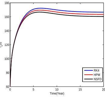
Figure 2. The plot shows the population of infected vector in the model.
0 5 10 15 20
60 80 100 120 140 160 180
Time(Year)
Iv
(t)
Figure 3. The plot represents the population of susceptible human
in the model.
0 5 10 15 20
2 4 6 8 10 12 14
Time(Year)
Sh
(t)
RK4 HPM NSFD
Figure 4. The plot represents the population of infected human in the model.
0 5 10 15 20
50 100 150 200
Time(Year)
Ih
(t)
Figure 5. The plot shows the population of recovered human in the
model.
0 5 10 15 20
0 20 40 60 80 100 120 140 160 180
Time(Year)
Rh
(t)
RK4 HPM NSFD
5. Conclusion
In this article, the solution of leptospirosis epidemic model is accomplished. We used a semi analytical approach for the solution of proposed model, that is Homotopy Perturbation Method. We obtained the solution by Homotopy Perturbation Method and compared the results with Runge-Kutta fourth order and NSFD method, which shows that Homotopy Perturbation Method is a powerful technique for the solution of such type of nonlinear epidemic models.
References
[1] S. Abbasbandy,Homotopy perturbation method for quadratic Riccati differential equation and comparison with Adomian decomposition method, Applied Mathematics and Computation,172 (2006), 485-490.
[2] S. Abbasbandy,Iterated he’s homotopy perturbation method for quadratic Riccati differential equation, Applied Mathematics and Computation,175(1) (2006), 581-589.
[3] N. Chitnis, T. Smith, and R. Steketee,A mathematical model for the dynamics of malaria in mosquitoes feeding on a heterogeneous host population, J. Biol. Dyn.,2(2008), 259-285. [4] M. Derouich and A. Boutayeb,Mathematical modelling and computer simulations of Dengue
fever, App. Math. Comput.,177(2006), 528-544.
[5] L. Esteva and C. Vergas,A model for dengue disease with variable human populations, J. Math. Biol.,38(1999), 220-240.
[6] D. D. Ganji and M. Rafei,Solitary wave solutions for a generalized Hirota–Satsuma coupled KdV equation by homotopy perturbation method, Physics Letters A,356(2006), 131-137. [7] J. H. He, The homotopy perturbation method for nonlinear oscillators with discontinuities,
Applied Mathematics and Computation,151(2004), 287-292.
[8] J. H. He,Comparison of homotopy perturbation method and homotopy analysis method, Applied Mathematics and Computation,156(2004), 527-539.
[10] J. H. He,Homotopy perturbation method for bifurcation of nonlinear problems, International Journal of Non-linear Science Numerical Simulation,6(2005), 207-208.
[11] J. H. He,Application of homotopy perturbation method to nonlinear wave equations, Chaos, Solitons and Fractals,26(2005), 695- 700.
[12] T. Khan, I. H. Jung, A. Khan, and G. Zaman, Classification and sensitivity analysis of the transmission dynamic of hepatitis B, Theoretical Biology and Medical Modelling, 14 (2017), 22-38.
[13] T. Khan, A. Khan, and G. Zaman,The extinction and persistence of the stochastic hepatitis B epidemic model, Chaos Solitons Fract,108(2018), 123-128.
[14] P. Pongsuumpun, T. Miami, and R. Kongnuy,Age structural transmission model for leptospiro-sis, The third International symposium on Biomedical engineering, 10-11 November 2008, 411-416.
[15] M. Rafei and D. D. Ganji,Explicit solutions of Helmholtz equation and fifth-order KdV equation using homotopy perturbation method, International Journal of Nonlinear Science and Numerical Simulation,7(2006), 321-329.
[16] A. M. Siddiqui, R. Mahmood, and Q. K. Ghori,Homotopy perturbation method for thin film flow of a fourth grade fluid down a vertical cylinder, Physics Letters A,352(2006), 404-410. [17] W. Triampo, D. Baowan, I. M. Tang, N. Nuttavut, J. Wong-Ekkabut, and G. Doungchawee,A
simple deterministic model for the spread of leptospirosis in Thailand, Int. J. Bio. Med. Sci.,2 (2007), 22-26.