Homotopy perturbation method for eigenvalues of non-definite
Sturm-Liouville problem
Farhad Dastmalchi Saei
Department of Mathematics, Tabriz Branch, Islamic Azad University, Tabriz, Iran. E-mail: [email protected]
Abstract In this paper, we consider the application of the homotopy perturbation method (HPM) to compute the eigenvalues of the Sturm-Liouville problem (SLP) which is called non-definite SLP. Two important Examples show that HPM is reliable method for computing the eigenvalues of SLP.
Keywords. Turning point, Sturm-Liouville, Homotopy perturbation method, Eigenvalues.
2010 Mathematics Subject Classification. 34L15.
1. Introduction
We study the indefinite Sturm-Liouville spectral problem
y00+ (λ r(x)−q(x))y= 0, a≤x≤b, (1.1)
y(a) =y(b) = 0,
defined on the interval [a, b] where λ is a real parameter, r(x), q(x) are real and integrable on [a, b]; moreover,
Z b
a
p
r+(t)dt >0, where r+(x) =max{r(x),0}. (1.2)
It follows from [5] that the spectrum of this problem is discrete and has no finite accu-mulation points; moreover, only finitely many eigenvalues lie the outside the real and imaginary axes. In what follows, we shall assume thatλis a positive parameter. This paper focuses on the Homotopy perturbation analysis (HPM), which has been intro-duced by He to solve approximately the differential equations [9] and [10]. Among numerical methods, the finite difference methods [3, 4], the variational methods and recently Homotopy perturbation analysis [2] are commonly referred as some tradi-tional and powerful methods for solving classic Sturm-Liouville problem. Of course, many new developments and improvements are often introduced [15, 17]. Scott [16] presented an initial-value method for SLP with non separated boundary conditions. Paine [14], Pryce [15] and Andrew [3] used finite difference scheme and asymptotic
Received: 3 October 2016 ; Accepted: 20 August 2018.
correction technique to solve classic SLP with Dirichlet boundary conditions. Ander-son and Hoog [4] extended the method of Paine to the general separated boundary conditions. C¸ elik [7] investigated the collocation method for approximating compu-tation of classic SLP eigenvalues by truncated Chebyshev series. C¸ elik and Gokmer [8] also applied the collocation method for computation of periodic SLP. Y¨ucel [18] applied the polynomial -based differential quadrature (PDQ) and Fourier expansion-based differential quadrature (FDQ) methods have been to compute the eigenvalues of periodic SLP. Chen and Ping Ma [6] proposed the Legendre-Galerkin-Chebyshev collocation method (LGCC) to compute the eigenvalues of SLP with many different boundary conditions. An improvement for Chebyshev collocation method in solving certain SLP is proposed by Yuan and et al [19]. They investigated SLP with two turning points and semi periodic boundary conditions.
At first, we mention the theory of higher order distribution of positive eigenvalues associated with problem (1.1), on the assumption that turning point is of arbitrary order. In particular, where the end points a or b is a zero of the weight functionr(x). At the end, we present numerical method both classic and non classic Sturm-Liouville problem. In this paper, we present Homotopy perturbation analysis for approximate computation of eigenvalues of SLP with Dirichlet boundary condition by focusing on a very important special case i.e. r(x) =xα orr(x) = (x−x
ν)α, in whichαmust be of odd order given the assumption of non-definiteness.
2. Eigenvalues of SLP:Theory and HPM
The theory of boundary eigenvalue problem (1.1) dates back to the pioneering research of R.G.D. Richardson and O. Haupt (see [13] and the references therein for a brief history and survey). The leading term in the asymptotic expansion of the real eigenvalues was the subject of the J¨orgens conjecture dating from 1964, a conjecture that was finally proved and extended in [5]. The thrust of this conjecture is that, once suitably relabeled, the positiveλ+
n eigenvalues admit the asymptotic estimate
λ+n ∼
n2π2
(Rabpr+(x)dx)2
, n→ ∞.
Mingarelli and Jodayree [16, 17] considered the caser(x) =xαon [a, b]. They showed following estimation
p
λ+n =
nπ−π
4 Rb
0 x
α/2 −
1 nπ{
4ν2−1
8R0bxα/2 −
1 2
Z b
0
q(x) xα/2}+O(
1 n2),
whereν= α1+2.
Also if we assume thatr(a) = 0 andr(x)>0 on (a, b] then
p
λ+n =
nπ+ (νπ
2 −
π
4) Rb
ax
α/2 −
1 nπ{
4ν2−1
8Rb
ax α/2 −
1
2H(b)}+O( 1
where
H(b) =
Z b
xν
(q(x) ˜ r(x)−
1 ˜ r3/4
d2
dx2(˜r
−1/4)) r˜
r12 dx,
and
˜ r= (dξ
dx)
2= 4r(x)
(α+ 2)2(ξ(x))α,
ξ(x) =
( −(Rxν
x (−r(t))
1/2dt)α2+2, x≤xν,
(Rxx
ν(r(t))
1/2dt)α2+2, x
ν≤x.
Without loss of generality, we consider problem
y00+ (λ r(x)−q(x))y= 0, 0≤x≤1, (2.2)
y(0) =y(1) = 0,
wherer(x) =xαorr(x) = (x−xν)α.
Since the homotopy perturbation method usually defines the given differential equa-tion in an operator form we will rewrite (1.1) in following form
A(y) =L(y) +N(y) =f(x).
HereL= d2
dx2,N(y) =−(λr(x)−q(x))yandf(x) = 0. Now we construct a homotopy υ(x, p) : Ω×[0,1]→R which satisfies
H(υ, p) = (1−p)[L(y)−L(y0)] +p[N(υ)−f(x)] = 0, p, x∈[0,1],
wherep∈[0,1] is embedding parameter,y0is an initial approximation, which satisfies
the boundary conditions. Obviously we have
H(υ,0) =L(y)−L(y0)],
H(υ,1) =A(y)−f(x).
Changing process ofpfrom zero to unity is just that of υ(x, p) fromy0 toy(x).
We assume that the solution of equation
H(υ, p) = (1−p)[L(y)−L(y0)] +p[N(υ)−f(x)] = 0, p, x∈[0,1], (2.3)
can be written as a power series inp,υ=υ0+pυ1+p2υ2+. . . .
3. Numerical examples and conclusions
In this section of the paper, for demonstrate the efficiency and accuracy of the HPM method, we give several numerical examples. Numerical results show that the HPM method is effective method for non-definite SLP.
Example 3.1. Consider the boundary value problem
y00+λxαy= 0, y(0) =y(1) = 0,
LetL(y) =y00and N(y) =λxαy. We also assume that
Y(x, p) =y0(x) +py1(x) +p2y2(x) +p3y3(x) +. . . .
By substituting of above in the differential equation and equating the coefficients of pwe obtain
coefficients ofp0:y000(x) = 0, y0(0) = 0,
coefficients ofp1:y100(x) +λxαy0(x) = 0, y1(0) =y10(0) = 0,
coefficients ofp2:y200(x) +λxαy1(x) = 0, y2(0) =y20(0) = 0,
.. .
If we solve the above equations we get
y0(x) =ax,
y1(x) =−aλxα+3/(α+ 2)(α+ 3),
y2(x) =aλ2xα+6/(α+ 2)(α+ 3)(α+ 5)(α+ 6),
y3(x) =−aλ3xα+8/(α+ 2)(α+ 3)(α+ 5)(α+ 6)(α+ 8)(α+ 9),
.. .
Therefore the solution of the problem is
y(x, λ) =a(x−λxα+3/(α+ 2)(α+ 3) +λ2xα+6/(α+ 2)(α+ 3)(α+ 5)(α+ 6)
−λ3xα+8/(α+ 2)(α+ 3)(α+ 5)(α+ 6)(α+ 8)(α+ 9) +· · ·).
If we consider special case by choosinga=λ5/6 andα= 1 then we have
y(x) =x1/2J1/3(2/3λ1/2x3/2).
To satisfy the other boundary condition we havey(1) = 0, which implies the eigen-values are the roots of J1/3(2/3λ1/2) = 0. On the other hand from [1] one can see
that the roots ofJν(z) are
jm∼β− α−1
8β −
4(α−1)(7α−31) 3(8β)3 −. . . ,
where
By insertingz= 2/3λ1/2x3/2andν = 1/3 we get
q
˜ λn =
3 2(nπ−
π 12) +
5 72(nπ− π
12)
+O( 1 n3).
On the other hand, by relation (2.1), the asymptotic distribution of eigenvalues sat-isfies
p
λn= 3 2(nπ−
π 12) +
5
48nπ +O( 1 n2).
From above we conclude that error of approximation satisfies
|pλn−
q
˜ λn|=
5 48nπ −
5 72(nπ− π
12)
+O( 1 n2).
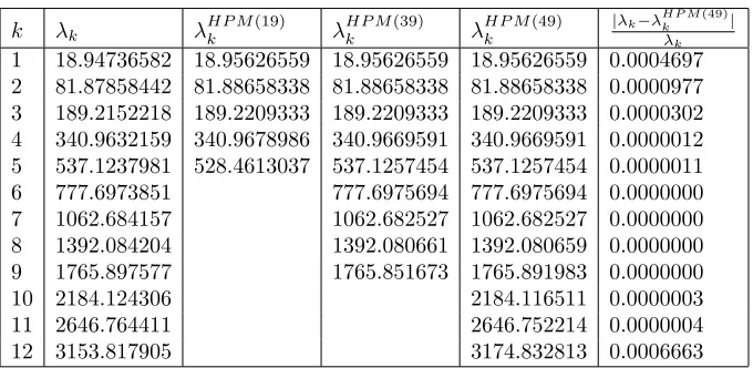
Table 1 shows comparison the eigenvalues for HPM method and asymptotic distri-bution of eigenvalues.
Table 1. Approximate solutions and error in Example3.1.
k λk λ
HP M(19)
k λ
HP M(39)
k λ
HP M(49)
k
|λk−λHP Mk (49)|
λk
1 18.94736582 18.95626559 18.95626559 18.95626559 0.0004697 2 81.87858442 81.88658338 81.88658338 81.88658338 0.0000977 3 189.2152218 189.2209333 189.2209333 189.2209333 0.0000302 4 340.9632159 340.9678986 340.9669591 340.9669591 0.0000012 5 537.1237981 528.4613037 537.1257454 537.1257454 0.0000011 6 777.6973851 777.6975694 777.6975694 0.0000000 7 1062.684157 1062.682527 1062.682527 0.0000000 8 1392.084204 1392.080661 1392.080659 0.0000000 9 1765.897577 1765.851673 1765.891983 0.0000000 10 2184.124306 2184.116511 0.0000003 11 2646.764411 2646.752214 0.0000004 12 3153.817905 3174.832813 0.0006663
Example 3.2. Consider the following SLP
y00+ (λxα−xβ)y= 0, y(0) =y(1) = 0,
whereα >0 andβ > α2. Note that the weight function vanishes at the left endpoint. By (2.1), we have
p
λn=k(nπ+ νπ
2 − π 4)−
1 nπ{
k(4ν2−1)
8 −
1
2(β−ν+ 2)}+O( 1 n2).
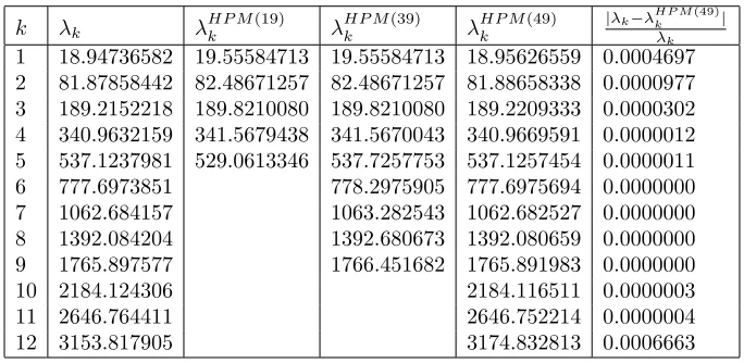
In the special case,α= 1, β= 2, the results are given in the Table 2. The relative error shows that position is better for large eigenvalues.
We also assume that
Y(x, p) =y0(x) +py1(x) +p2y2(x) +p3y3(x) +. . . .
By substituting of above in (3.1) and equating the coefficients ofpwe obtain
coefficients ofp0:y00
0(x) = 0, y0(0) = 0,
coefficients ofp1:y00
1(x) + (λx−x2)y0(x) = 0, y1(0) =y01(0) = 0,
coefficients ofp2:y00
2(x) + (λx−x2)y1(x) = 0, y2(0) =y02(0) = 0,
.. .
If we solve the above equations we get
y0(x) =ax,
y1(x) =ax5/4.5−aλx4/3.4,
y2(x) =ax9/4.5.8.9 +aλ2x7/3.4.6.7−5aλx8/60.42,
.. .
Therefore the solution of the problem is
y(x, λ) =a(x+x5/4.5−λx4/3.4 +x9/4.5.8.9 +λ2x7/3.4.6.7−5λx8/60.42 +· · ·).
Table 2 shows comparison the eigenvalues for HPM and asymptotic distribution of eigenvalues.
Table 2. Approximate solutions and error in Example3.2.
k λk λ
HP M(19)
k λ
HP M(39)
k λ
HP M(49)
k
|λk−λ HP M(49)
k |
λk
4. Conclusions
In this paper, we investigate the HPM for approximation of eigenvalues of non-definite SLP with Dirichlet boundary conditions. One of the main advantage of this method is that the approximate trivial solution (y0(x)) will spontaneously be satisfy
in Dirichlet boundary conditions. The numerical examples showed that the HPM is efficient and considerable.
References
[1] M. Abramowitz and J. A. Stegun,Hand book of Mathematical Function, Appl, Math, Ser. no. 55, U.S Govt. Printing office, Washington, D. C., 1964.
[2] A. Abbasbandy and A. Shirzadi,A new application of the homotopy analysis method: solving the Sturm-Liouville problems, Commun. Nonlinear. Sci. Numer. Simulat,16(2011), 112–126. [3] A. L. Andrew,Correction of Numerov’s eigenvalue estimates, Numer. Math., 47(1985), 289–
300.
[4] F. R. Anderson and D. Hoog,On the correction of finite difference eigenvalue approximations for the Sturm-Liouville problems with general boundary conditions, Bht,24(1984), 401–412. [5] F. V. Atkinson and A. Mingarelli,Asymptotics of the number of zeros and the eigenvalues of
general weighted Sturm-Liouville problems, Journal der reinen und angewandten Mathematik,
395(1986), 380–93.
[6] L. Chen and H. P. Ma,Approximate solution of the Sturm-Liouville problems with Legendre-Galerkin-Chebyshev collocation method, Math. of Computation,74(252) (2005), 1793–1801. [7] I. C¸ elik, Approximate computation of eigenvalues with Chebychev collocation method, Appl.
Math. Comp,168(2005), 125–134.
[8] I. C¸ elik and G. Gokmer,Approximate solution of periodic Sturm-Liouville problems with Cheby-chev collocation method, Appl. Math. Comp,170(2005), 285–295.
[9] H. J. He,Homotopy perturbation method for solving boundary value problems, Physics Letters A,350(1-2) (2006), 87–88.
[10] H. J. He, Homotopy perturbation technique, Computer Methods in Applied Mechanics and Engineering,78(3-4) (1999), 257–262.
[11] A. Jodayree Akbarfam and A. Mingarelli,Higher-order asymptotic distribution of the eigenval-ues of nondefinite Strurm -Liouville problems with one turning point, J. Com. App. Math.,149
(2002), 423–437.
[12] A. Jodayree Akbarfam and A. Mingarelli,Higher-order asymptotic of the eigenvalues of Strurm-Liouville problems with a turning point of arbitrary order, Cana. App. math. Quart.,12(2004), 35–60.
[13] A. B. Mingarelli,Asymptotic distribution of eigenvalues of non-definit Sturm-Liouville problems in Ordinary differential equations and operators, W. N. Everitt and R. T. Lewis(eds), Lecture Notes in Math., Springer-verlag, berlin,1032(1983), 375–383.
[14] J. W. Paine, D. Hoog, and R. S. Anderssen,On the correction of finite difference eigenvalue approximations for Sturm-Liouville problems, Computing,26(1981), 123–139.
[15] J. D. Pryce,Numerical solution of Sturm-Liouville problems, Clarendon, Oxford.
[16] M. R. Scott,Invariant embedding and thecalculating of eigenvalues for differential equations with nonseperated boundary conditions, J. Optimiz. Theory. Appl.,12(4) (1973), 355–366. [17] S. Somali and V. Oger,Improvment of eigenvalues of Sturm-Liouville problems with t-periodic
boundary conditions,180(2005), 433–441.
[18] U. Y¨ucel,Approximate eigenvalues of periodic Sturm-Liouville problems using differential quad-rature method, Appl. Math. Scie.,1(25) (2007), 1217–1229.