in the population sciences published by the Max Planck Institute for Demographic Research Konrad-Zuse Str. 1, D-18057 Rostock · GERMANY www.demographic-research.org
DEMOGRAPHIC RESEARCH
VOLUME 22, ARTICLE 12, PAGES 289-320
PUBLISHED 05 MARCH 2010
http://www.demographic-research.org/Volumes/Vol22/12/ DOI: 10.4054/DemRes.2010.22.12
Research Article
The effects of shocks in early life mortality
on later life expectancy and mortality
compression: A cohort analysis
Mikko Myrskylä
© 2010 Mikko Myrskylä.
This open-access work is published under the terms of the Creative Commons Attribution NonCommercial License 2.0 Germany, which permits use, reproduction & distribution in any medium for non-commercial purposes, provided the original author(s) and source are given credit.
1 Introduction 290
2 Background 290
3 Anticipated effects of cohort mortality shocks 295
4 Data, variables and methods 297
4.1 Data and variables 297
4.2 Methods 299
4.3 Characteristics of the data 301
5 Results 303
5.1 Early life mortality and life expectancy 303
5.2 Early life mortality and compression of mortality 309
5.3 Sensitivity analysis 312
6 Discussion 312
7 Acknowledgements 315
The effects of shocks in early life mortality on
later life expectancy and mortality compression:
A cohort analysis
Mikko Myrskylä1
Abstract
I study how shocks in cohort-level early life conditions, as represented by deviations from trend in mortality before age 5, affect later mortality. I use data for six European countries and find that shocks that increase infant mortality decrease later life expectancy between ages 5-30. The effect is strong for England and Wales but small or insignificant for other countries. Shocks that increase mortality at ages 1-5 increase life expectancy between ages 5-30 and compress the mortality distribution. For both shocks the effects are weak at older ages. These results suggest that early life conditions have a transitory effect and potentially only little influence on old-age mortality.
1. Introduction
Cohorts born in different periods separated by short time interval often experience different mortalities over their life course. These differences, which are sometimes interpreted as signifying “cohort effects” on mortality, are well documented (for example, Wilmoth, Vallin and Caselli 1990) but the sources of these differences remain uncertain.
Early life conditions are one potential source of the differences in cohort mortality. At the individual-level, it has been shown that early life conditions and adult health and mortality are linked (Case, Fertig and Paxson 2005; Hayward and Gorman 2004; Preston, Hill and Drevenstedt 1998). It is, however, less clear whether a cohort-level link from early life conditions to later life mortality exists, and if so, whether the link is strong enough to explain cohort level differences in adult- and old-age mortality. Moreover, disentangling the early life effects, effects that cumulate over the life course and period effects is methodologically challenging. Consequently, evidence regarding the importance of cohort’s early life conditions on later life mortality is mixed and continues to be debated (Elo and Preston 1992; Kannisto, Christensen and Vaupel 1997; Bengtsson and Lindstrom 2000; Doblhammer 2004; Finch and Crimmins 2004; Barbi and Vaupel 2005; Catalano and Bruckner 2006; Bengtsson and Mineau 2009; Gagnon and Mazan 2009; Bruckner and Catalano 2009; van den Berg, Doblhammer and Christensen 2009).
This paper uses historical time series for six European countries to analyze how early life conditions, proxied by cohorts’ mortality at ages below 5, predict later life cohort-level mortality. The results show that shocks causing above trend mortality during the first year of life increase mortality at ages 5-30, and that shocks causing above-trend mortality at ages 1-5 decrease mortality at ages 5-30 and compresses the age at death distribution. The effects are small at older ages. Gender differences are also small. The findings are consistent with the emerging literature suggesting that cohort’s old-age mortality is not strongly linked to cohort’s early life mortality (Bruckner and Catalano 2009; Gagnon and Mazan 2009; van den Berg et al. 2009) but could be linked to other indicators of early life conditions such as the state of the business cycle at birth (van den Berg, Lindeboom and Portrait 2006; van den Berg et al. 2009).
2. Background
individuals. During recent decades, interest in the effects of early life conditions on adult health and mortality has been revitalized by Barker and colleagues (Barker et al. 2002; Barker 1992, 1994; Eriksson et al. 1999). The influential “Barker theory” or “fetal origins of adult disease theory” predicts that cohort-level mortality differences may, at least partly, be explained by the cohorts’ early life conditions. While the Barker theory focuses on in utero nutrition, it is possible that also other early life factors, such as exposure to disease or macro-economic conditions (which could be a proxy for nutrition or disease), matter. In addition, it may be that also other stages of early life, especially the first years after birth, are sensitive to early life experiences.
Evidence regarding the cohort-level links between early life conditions and later life health and mortality, however, is mixed. Almond (2006) analyses U.S. data and finds lower educational attainment and income for those in utero during the 1918 influenza when compared to the neighboring birth cohorts. Cohen and Tillinghast (2009), however, analyze data from 24 countries and find no long-term mortality effects for prenatal or neonatal exposure to the 1918 influenza. The study by Almond identifies the timing of exposure more accurately than Cohen and Tillinghast, which may explain the difference in results, but it is also possible that old-age health but not mortality is sensitive to early life exposure to disease. Studies focusing on the long-term impact of early life nutritional deprivation have produced at least as mixed results. Studies on the Finnish famine of 1866-1868 (Kannisto et al. 1997) and the Dutch famine of 1944-1945 (Painter et al. 2005) have found no association between nutritional deprivation early in life and later mortality. Van den Berg et al. (2007) analyze the effects of 1846-47 Dutch potato famine and find that those who were exposed to the famine in utero may have had increased mortality at ages above 50, but for women no effects are found. In contrast to these results, Fogel (2004) and Costa and Lahey (2005) attribute much of the decline in old age mortality to improved nutrition.
families or household heads to migrate in search for jobs or better life; this could affect later life health of those born in a recessions through various mechanisms.
This paper focuses on the cohort-level links between early life conditions and later life mortality using cohort-level mortality as a proxy for early life conditions. Existing evidence regarding these links is inconclusive. Finch and Crimmins (2004), Barbi and Vaupel (2005) and Crimmins and Finch (2006a, 2006b) study the link between cohorts’ early life and late life mortality, and find that these are strongly and positively correlated. The correlations presented, however, may be spurious since both the dependent and independent variables are subject to trends. One way to deal with the problem arising from trends in the variables is to de-trend the variables before analysis. This approach was pioneered by Bengtsson and Lindström (2000, 2003), who analyze the association between de-trended infant and child mortality at the time of birth and de-trended mortality at older ages, and find that disease load during the first year of life (proxied by early life mortality conditions) is associated with higher mortality later in life. Bengtsson and Lindstöm use the Hodrick-Prescott filter (Hodrick and Prescott 1997) in de-trending, and this method has become a common tool in demography (for example, van den Berg et al. 2009; Gagnon and Mazan 2009).
Catalano and Bruckner (2006) use a similar de-trending approach to study the association between cohort’s early life and later mortality. They use national level historical mortality data for Sweden, Denmark, and England and Wales. Instead of the Hodrick-Prescott filter, Catalano and Bruckner de-trend the early and later life mortality variables using ARIMA (Auto-Regressive Integrated Moving Average) models (Box and Jenkins 1970) with autoregressive lags up to 10 and moving average lags up to 8. Catalano and Bruckner find that higher than expected mortality during the first five years of life may decrease life expectancy at age 5 by as much as 1.75 years, and that the effect is stronger for men than for women. The result suggests that, at the cohort level, early life conditions play an important role in determining later mortality. The effect (1.75 years), however, is difficult to interpret because it corresponds to the difference between minimum and maximum in the independent variable, not to a one standard deviation difference in the independent variable. The significance of the results may also be exaggerated as the statistical tests are one-sided. A priori high early life mortality could also potentially increase later life expectancy through selection.
mortality have increased adult mortality. The magnitude of the effect is sizable; for example in the 2009 paper that analyses mortality at ages above 55 for 1766-1839 birth cohorts, those born in years with very high infant mortality (deviation from trend in the highest decile) face up to 43% higher old-age mortality than those born in times of lower infant mortality.
Others who have used largely similar study designs that Bengtsson et al. have developed have generally failed to find links between being born in times of high mortality and later mortality. van den Berg et al. analyze the links between being born during times of high mortality and later adult mortality (van den Berg, Lindeboom and Portrait 2006; van den Berg, Doblhammer and Christensen 2009).2 The 2006 paper uses data on Dutch 1812-1912 birth cohorts with mortality follow-up until 2000, and finds no substantially or statistically significant links between infant mortality at the time of birth and later mortality. The 2009 paper uses Danish twin registry to analyze the links between early and later life mortality for 1872-1906 birth cohorts, and finds no evidence for any links between mortality conditions at birth and adult mortality. Gagnon and Mazan (2009) use essentially the same analytical design that Bengtsson et al. and van den Berg et al. use to analyze the effects of infant mortality on later adult mortality in a pre-industrial French-Canadian population. The birth cohorts are from 1680 to 1750. The demographic context in the study by Gagnon and Mazan is unique as the population experiences stable or increasing rather than decreasing mortality over time. Gagnon and Mazon estimate the associations both with and without de-trending3 the early life mortality variable. In both cases the links between early and later life mortality are statistically and substantially small.
Finally, in a follow-up to the Catalano and Bruckner 2006 paper, Bruckner and Catalano estimate the cohort-level links between de-trended mortality early in life and de-trended later mortality (Bruckner and Catalano 2009).4In contrast to the 2006 paper which analyzed only life expectancy at age 5, the 2009 paper decomposes the effects of early life mortality conditions on later mortality by age. The data is the same data as it
2 While the main focus of these papers is on the effects of economic conditions early in life, the effects of
mortality conditions early in life on later mortality is also analyzed carefully.
3 The need for de-trending is not very strong in this case as the trends are weak, and inexistent secular trends
in period conditions can not confound the results.
4 Certain features of the study design and some of the results of the current paper are similar to Bruckner and
Catalano (2009), henceforth BC2009. The current paper was developed independently of BC2009. The
current paper was submitted in July 2008. I learned about the still forthcoming BC2009 on January 16th 2009
was in the 2006 paper, and the methods including the ARIMA-model based de-trending are also similar. The age-decomposition indicates that the effects of early life exposure to conditions that elevate mortality rates on later life mortality are expressed mainly at young ages (below 20); at old ages the effects are substantially and statistically small.
To summarize, the research concerning the link between mortality conditions early in life, which should be taken as a broad proxy for the epidemiologic environment, and later mortality is inconclusive. The results in studies that find a very strong association between cohort’s mortality early in life and later mortality using aggregate national-level mortality data may be confounded by changing period conditions (Barbi and Vaupel 2005; Crimmins and Finch 2006a, 2006b; Finch and Crimmins 2004; Kermack et al. 1934, 2001). Studies that remove the potentially confounding period effect using de-trending techniques mostly find a weak or no link between cohort-level early life mortality and later mortality (Gagnon and Mazan 2009; van den Berg et al. 2006, 2009; Bruckner and Catalano 2009). An exception is the series of studies using data from 18th -19th century rural Sweden (Bengtsson and Broström 2009; Bengtsson and Lindstrom 2000, 2003). These careful analyses by Bengtsson and colleagues identify the timing of above or below-trend infant mortality on a regional level and suggest that early life mortality conditions do matter for adult mortality, or did at least in the populations analyzed. It is however not clear why the results are so different from the studies by van den Berg et al. (2006, 2009) and Gagnon and Mazan (2009). In addition, if there are long-lasting links between cohort level early life conditions, and later life mortality, it is not fully known how long-lasting these links are – the results by Bruckner and Catalano suggest that the majority of the effect may disappear by age 30.
The current paper contributes to the knowledge on cohort-level links between early life conditions and later life mortality using historical time series for six European countries (Denmark, England and Wales, Finland, the Netherlands, Sweden and Switzerland). The paper builds on Catalano and Bruckner (2006) and uses some methodological features introduced to demography by Bengtsson and Lindstrom (2000). I analyze the links between deviations from trend in mortality before age five and de-trended later mortality. I break mortality before age 5 into infant (age 0) and early childhood (ages 1-5) mortality, this decomposition allows me to analyze in more detail what are the sensitive periods of life. As dependent variables, I use conditional life expectancy. In order to study at what stages of the life course mortality responds to early life conditions, I measure conditional life expectancy at ages 5-30, 30-50, 50-70, and 70-90.
would be reached anytime soon (Edwards and Tuljapurkar 2005; Kannisto 2000; Wilmoth and Horiuchi 1999). Most research, however, has focused on period measured of mortality compression. Van den Berg, Lindeboom and Portrait (2006) show that mortality differentials across social classes are exacerbated for cohorts born during recessions, but there are no studies analyzing how cohort level compression of mortality depends on cohort’s early life mortality. In this paper I analyze how interquartile range in age at death, a compression measure suggested by Wilmoth and Horiuchi (1999), responds to shocks in cohort’s early mortality.
All the analyses use the Hodrick-Prescott filter to break observed time series into a trend and residual. Analysis of the correlations in the residuals, or shocks, allows me to answer the question how does cohort’s mortality at ages above 5 depend on mortality experience before age 5.
3. Anticipated effects of cohort mortality shocks
I term environmental shocks that influence mortality as mortality shocks. These may be related to cohort-level later mortality through selection, scarring or induced immunity.5 Assume a cohort has a robustness distribution that could be, for example, gamma or Gaussian. The robustness distribution is directly linked to age at death distribution so that high values of robustness reflect high expected age at death and low values of robustness reflect low expected age at death. Likewise, the variance of the robustness distribution is linked to the compression of mortality so that the higher the variance in robustness the lower the mortality compression and vice versa. I outline briefly what could be expected to happen to the mean and variance of the robustness distribution after an adverse mortality shock, such as a famine, disease epidemic or war that results in excess mortality in cohort’s early life. Table 1 summarizes these effects.
5 Preston, Hill and Drevensted (1998) present a related typology of four mechanisms that relate the risk of
First, an early life cohort mortality shock may have a scarring effect that lowers mean robustness for the surviving cohort thus increasing later mortality and lowering the expected age at death. This effect applies to both individuals and cohorts. Second, an early life cohort mortality shock may act selectively, killing the weakest. This would results in a lowering of the left tail of the age at death distribution for the survivors. The effect of such selection on the mean of the robustness distribution would be positive, increasing the expected age at death for the surviving cohort. Third, an early life cohort mortality shock may induce immunity, increasing the mean of the robustness distribution and the expected age at death. The sorting out of the selection and acquired immunity effects is difficult in practice, as the prevalence of high immunity in a surviving cohort may be due to acquired immunity or the selection of the not-immune out of the cohort. Note also that only shocks with a scarring effect or immunity inducing effect influence individual mortality. Selection, in turn, does not affect the surviving individuals’ mortality but does affect cohort-level mortality.
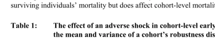
Table 1: The effect of an adverse shock in cohort-level early life conditions on
the mean and variance of a cohort’s robustness distribution
Type of effect Change in mean Change in variance
Selection/Culling + -
Scarring - +/-
Immunity + +/-
Total ? ?
Note: The robustness distribution is directly linked to age at death distribution so that high values of robustness reflect high expected age at death and low values of robustness reflect low expected age at death. Similarly, large (small) variance in robustness reflects large (small) variance in age at death.
To summarize, conceptually shocks in cohort’s early life mortality conditions may either increase or decrease both longevity and variation in age at death for the survivors of the same cohort. It is also unclear at what ages mortality would be altered by an early life cohort shock. This paper analyses the links between cohort’s early and later mortality, and hopefully sheds light on which of the three within-cohort effects dominates: selection, scarring, or immunity.
4. Data, variables and methods
4.1 Data and variables
I use time series data on the numbers of deaths and years of exposure by cohort for Denmark (cohorts born between 1835 and 1915), England and Wales (1841-1915), Finland (1878-1915), the Netherlands (1850-1915), Sweden (1751-1915) and Switzerland (1876-1915). The data source is the Human Mortality Database(University of California, Berkeley (USA) and the Max Planck Institute for Demographic Research (Germany) 2008).
4m1
As an indicator for early life conditions I use mortality at ages 0 and 1-5,6 denoted by 1m0 and and calculated as
n x
n x D PY
nDx
nmx= (1)
where is the number of deaths and nPYx is person-years lived between ages x and x n+ .
I measure a cohort’s longevity by conditional life expectancy. This is the average number of years lived between ages x and x n+ for those who survive to x, denoted by nex and calculated as
n x
x PY
l
nPYx
n xe = , (2)
where is as in (1) and lx is the number of people who survived to x. For each cohort I calculate 85 5e , 25e5, 20 30e , 20 50e and 20 70e .7
For mortality compression, there are several alternative indicators (Kannisto 2000; Wilmoth and Horiuchi 1999). Wilmoth and Horiuchi (1999) show that these are highly correlated with each other, thus the choice of the indicator is not likely to be critical. I use interquartile range in age at death conditional on surviving to age x. This measure is easy to calculate and interpret, and recommended by Wilmoth and Horiuchi (1999). The measure is also convenient for cohort studies because one can calculate the interquartile range after observing only 75% of the deaths. This means that the interquartile range is fully observed for cohorts born as late as 1915, the youngest cohort included in this study. I denote the conditional interquartile range in age at death for those who survived to age x by iqrx. The value of iqx
r is calculated the usual way as the difference between the third and first quartiles in age at death for those who
4m1
20 90e
6 Also mortality at ages 0-5 was analyzed. The results were similar to those obtained with , but slightly
attenuated.
7 Also
10 and were analyzed. The results were consistent with those obtained using age 90 as the
upper limit. I use age 90 as the upper limit instead of 110 because this allows me to use 20 more cohorts for each country.
survive to age x. For each cohort I calculate and , the interquartile range in age at death for those who survive to ages 5 or 30.
5
iqr iqr30 8
4.2 Methods
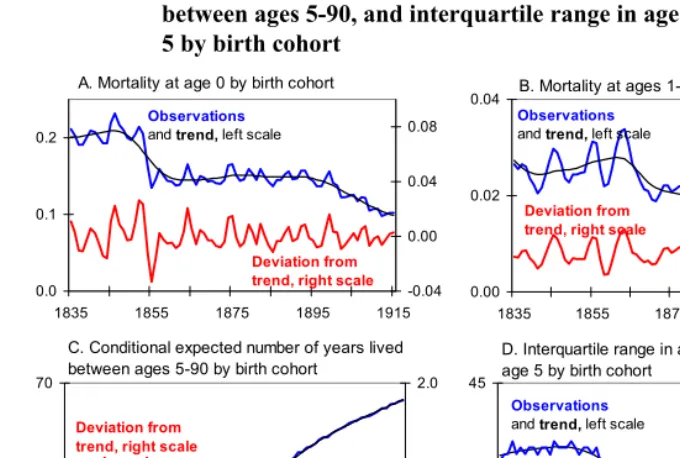
All the time series of this study are subject to trends: life expectancies are increasing, mortality rates are decreasing, and mortality is being compressed (see Figure 1). When analyzing the associations between variables which are subject to trend it is often useful to start by de-trending the variables. The reason for this is that regressing a variable with a trend on another variable with a trend may yield statistically significant results, irrespective of the true nature of their associations (Hendry 1980). Therefore I decompose the series into trend and deviation from trend, and model the deviations from trend. I de-trended each of the series over cohorts using the Hodrick–Prescott filter (Hodrick and Prescott 1997) with a smoothing parameter λ=100, a standard choice for annual data (Maravall and del Río 2007).9 Figure 1 shows the data (original series, estimated trend and residuals) for Denmark for selected variables. Panels A and B of Figure 1 show the independent variables, mortality at ages 0 and 1-5. The black line is for the original series, the blue line is for the estimated trend, and the red line is for the deviations from trend, or shocks, in early life mortality. Panels C and D of Figure 1 show the data for conditional life expectancy at ages 5-90 and interquartile range in age at death above age 5. The graphs are qualitatively similar for other countries (not shown), so that mortality and interquartile range in age at death are both decreasing over cohorts, and life expectancy is increasing.
8 The analysis was also done with conditional standard deviation in age at death as the dependent variable.
The results were somewhat stronger than they are with the interquartile range, but qualitatively not different.
9 Two other smoothing parameters were also analyzed, λ=6.25, suggested by Ravn and Uhlig (2002) and
1600
λ= , often used for quarterly data. The larger the value of λ the less the smoothing. Therefore the
estimated residuals did change when λ was changed. The estimates for the model parameters, however, were
Figure 1: Denmark: Mortality at ages 0 and 1-5, conditional life expectancy between ages 5-90, and interquartile range in age at death above age 5 by birth cohort
A. Mortality at age 0 by birth cohort
0.0 0.1 0.2
1835 1855 1875 1895 1915
-0.04 0.00 0.04 0.08
B. Mortality at ages 1-4 by birth cohort
0.00 0.02 0.04
1835 1855 1875 1895 1915
-0.01 0.01 0.03 Observations
and trend, left scale Observations
and trend, left scale
Deviation from trend, right scale Deviation from
trend, right scale
C. Conditional expected number of years lived between ages 5-90 by birth cohort
50 60 70
1835 1855 1875 1895 1915
-2.0 0.0 2.0
Observations and trend, left scale
D. Interquartile range in age at death above age 5 by birth cohort
15 30 45
1835 1855 1875 1895 1915
-2.0 0.0 2.0 4.0 6.0 Observations
and trend, left scale Deviation from
trend, right scale
Deviation from trend, right scale
Source: Observations: Human Mortality Database; trend and deviation from trend: own calculations.
I estimate the effects of early childhood mortality shocks on later mortality using a model
Y =β′X+ε
Y e5
20 50e 70
30 X
, (3)
where is the dependent variable (for life expectancy, deviation from trend in 85 ,
, , , and and for compression of mortality, deviation from trend in and
iqr
) and is the vector of predictors. The first set of models includes only infant mortality shocks, so25 5e 20 30e 20e
5
iqr
0
β
=
β . The second set of models include only early childhood mortality shocks, so β=β1 4− . The last set of models has both shocks, so
. The models are estimated for a pooled data including all countries, and also separately for each country and for both genders. The three sets of models are used
(
β β0, 1 4−)
=
because I wanted to study the explanatory power of both infant and early childhood mortality shocks, and because even after de-trending, these shocks may be so correlated that joint estimation of the effects is inaccurate.
I estimate the Model (3) by ordinary least squares (OLS). I studied the sensitivity of the results to the OLS assumptions by estimating the models with auto-correlated residuals with lags up to 5, selecting the optimal number of lags with the generalized Durbin-Watson test. The results were only marginally different from the OLS results, so only the OLS results are presented here.
0 1
The model (3) controls implicitly for period changes in two ways: first, cohorts born within a short period are compared to each other, thus keeping the period factor almost constant, and second, the remaining influence of changing periods is removed by de-trending. The coefficients of model (3) are related to Table 1 as follows. If mortality shocks in childhood were negatively correlated with later life expectancy (β β, 4 0
0 1
− < ), then the scarring effect must dominate the selection and immunity effects (see Table 1). If mortality shocks were positively correlated with later life expectancy (β β, −4>0), then those who survive would be on average less frail than those who die as a result of the mortality shocks. This would be consistent both with selection and immunity theories. When the response variable is interquartile range in age at death, negative coefficients would be consistent with all three theories, and positive coefficients with scarring and immunity theories.
4.3 Characteristics of the data
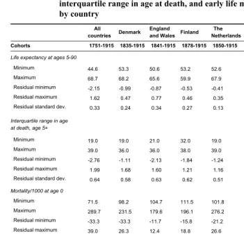
Table 2 shows the range of the data and residual standard deviation (standard deviation for the de-trended data) for some key variables. The number of cohorts by country varies from 165 (Sweden, 1751 to 1915) to 38 (Finland, 1878 to 1915). Generally, the longest series of cohorts have the lowest minimum life expectancies, highest maximum mortality rates, and largest residual variation. This pattern is due to decreasing mortality and decreasing variance over time.
Table 2: Minimum and maximum for levels and minimum, maximum and standard deviation for de-trended residuals for life expectancy, interquartile range in age at death, and early life mortality variables by country
All
countries Denmark
England and Wales Finland
The
Netherlands Sweden Switzerland Cohorts 1751-1915 1835-1915 1841-1915 1878-1915 1850-1915 1751-1915 1876-1915
Life expectancy at ages 5-90
Minimum 44.6 53.3 50.6 53.2 52.6 44.6 57.8
Maximum 68.7 68.2 65.6 59.9 67.9 68.7 68.6
Residual minimum -2.15 -0.99 -0.87 -0.53 -0.41 -2.15 -0.33
Residual maximum 1.62 0.47 0.77 0.46 0.35 1.62 0.53
Residual standard dev. 0.33 0.24 0.34 0.27 0.13 0.43 0.17
Interquartile range in age at death, age 5+
Minimum 19.0 19.0 21.0 32.0 19.0 19.0 21.0
Maximum 39.0 36.0 36.0 38.0 39.0 39.0 29.0
Residual minimum -2.76 -1.11 -2.13 -1.84 -1.24 -2.76 -1.29
Residual maximum 1.99 1.68 1.60 1.21 1.16 1.99 1.24
Residual standard dev. 0.64 0.58 0.63 0.62 0.51 0.75 0.52
Mortality/1000 at age 0
Minimum 71.5 98.2 104.7 111.5 101.8 71.5 90.5
Maximum 289.7 231.5 179.6 196.1 276.2 289.7 254.5
Residual minimum -33.3 -33.3 -11.7 -15.8 -21.2 -33.3 -13.9
Residual maximum 39.0 26.3 12.4 18.8 26.6 39.0 13.8
Residual standard dev. 9.4 9.5 4.9 7.4 10.4 10.6 6.5
Mortality/1000 at ages 1-5
Minimum 6.2 6.2 15.1 18.8 10.9 8.3 7.7
Maximum 53.7 33.8 40.7 42.8 45.5 53.7 23.4
Residual minimum -13.0 -5.4 -2.9 -6.0 -3.8 -13.0 -2.8
Residual maximum 7.5 6.2 3.6 5.9 5.2 7.5 2.3
Residual standard dev. 2.3 2.1 1.0 2.9 1.6 2.9 1.0
Source: Levels: Human Mortality Database, residuals: own calculations.
(Denmark). The range of residual variation in infant mortality is from 4.9 (England and Wales) to 10.6 (Sweden), and in childhood mortality from 1.0 (England and Wales, Switzerland) to 2.9 (Finland, Sweden) deaths per 1000 person years. It is not surprising to see higher residual variation in the early life mortality rates than in the dependent variables, since the dependent variables are summary measures over time. For such variables, good and bad times tend to even out, decreasing variance.
5. Results
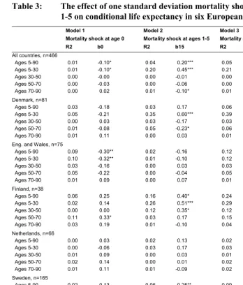
Section 5.1 analyzes the effects of mortality shocks on conditional life expectancy; Section 5.2 focuses on mortality compression; and Section 5.3 discusses sensitivity analyses. In Sections 5.1 and 5.2, the tables present three models: Model 1 has only infant mortality as the predictor, Model 2 uses only early childhood mortality, and Model 3 shows both. The coefficients are standardized to show the effect of one standard deviation positive shock (higher than expected mortality) in the predictor variable. As the models are linear, one standard deviation negative shock (lower than expected mortality) would have the same effect but with the opposite sign.
5.1 Early life mortality and life expectancy
Model 1,Table 3 regresses de-trended conditional life expectancy on infant mortality.
Overall, the model explains very little of variation of life expectancy at any ages. In the pooled regression which combines all countries ranges from 0.00 to 0.01, and in the country specific analyses the highest is 0.11 (Finland, ages 50-70).
2
R
2
R
Table 3: The effect of one standard deviation mortality shocks at ages 0 and 1-5 on conditional life expectancy in six European countries
Model 1 Model 2 Model 3
Mortality shock at age 0 Mortality shock at ages 1-5 Mortality shocks at ages 0 and 1-5
R2 b0 R2 b15 R2 b0 b15
All countries, n=466
Ages 5-90 0.01 -0.10* 0.04 0.20*** 0.05 -0.10* 0.20***
Ages 5-30 0.01 -0.10* 0.20 0.45*** 0.21 -0.11** 0.45***
Ages 30-50 0.00 -0.00 0.00 -0.01 0.00 -0.00 -0.01
Ages 50-70 0.00 -0.03 0.00 -0.06 0.00 -0.03 -0.06
Ages 70-90 0.00 0.02 0.01 -0.10* 0.01 0.02 -0.10*
Denmark, n=81
Ages 5-90 0.03 -0.18 0.03 0.17 0.06 -0.17 0.16*
Ages 5-30 0.05 -0.21 0.35 0.60*** 0.39 -0.18* 0.59***
Ages 30-50 0.00 0.03 0.03 -0.17 0.03 0.02 -0.17
Ages 50-70 0.01 -0.08 0.05 -0.23* 0.06 -0.09 -0.23*
Ages 70-90 0.01 0.11 0.00 0.03 0.01 0.11 0.04
Eng. and Wales, n=75
Ages 5-90 0.09 -0.30** 0.02 -0.16 0.12 -0.31** -0.16
Ages 5-30 0.10 -0.32** 0.01 -0.10 0.12 -0.32** -0.11
Ages 30-50 0.03 -0.16 0.00 0.03 0.03 -0.16 0.03
Ages 50-70 0.05 -0.22 0.00 -0.04 0.05 -0.22 -0.05
Ages 70-90 0.01 0.09 0.00 0.07 0.01 0.09 0.07
Finland, n=38
Ages 5-90 0.06 0.25 0.16 0.40* 0.24 0.27 0.42***
Ages 5-30 0.02 0.14 0.26 0.51*** 0.29 0.16 0.52***
Ages 30-50 0.00 0.00 0.12 0.35* 0.12 0.02 0.35*
Ages 50-70 0.11 0.33* 0.03 0.17 0.15 0.34* 0.19
Ages 70-90 0.03 0.19 0.01 -0.10 0.04 0.18 -0.09
Netherlands, n=66
Ages 5-90 0.00 0.03 0.02 0.13 0.02 0.04 0.14
Ages 5-30 0.00 -0.06 0.03 0.17 0.03 -0.04 0.17
Ages 30-50 0.01 0.09 0.00 0.03 0.01 0.09 0.04
Ages 50-70 0.02 0.14 0.00 0.01 0.02 0.14 0.03
Ages 70-90 0.01 0.11 0.01 -0.09 0.02 0.10 -0.08
Sweden, n=165
Ages 5-90 0.02 -0.13 0.06 0.25** 0.09 -0.15* 0.27***
Ages 5-30 0.01 -0.10 0.25 0.50*** 0.27 -0.15* 0.51***
Ages 30-50 0.00 0.01 0.02 -0.14 0.02 0.03 -0.15
Ages 50-70 0.00 -0.03 0.00 -0.06 0.00 -0.03 -0.06
Ages 70-90 0.00 -0.06 0.03 -0.17* 0.03 -0.04 -0.17*
Switzerland, n=41
Ages 5-90 0.02 0.14 0.02 0.13 0.04 0.17 0.15
Ages 5-30 0.06 0.24 0.02 0.13 0.07 0.22 0.11
Ages 30-50 0.00 0.00 0.00 -0.07 0.00 0.01 -0.07
Ages 50-70 0.00 0.07 0.00 0.04 0.01 0.06 0.04
Ages 70-90 0.00 0.02 0.01 -0.09 0.01 0.03 -0.09
Notes: Model 1: b0 is the effect of a 1 SD increase in de-trended cohort mortality at age 0. Model 2: b15 is the effect of a 1 SD increase in de-trended cohort mortality at ages 1-5. Model 3: b0 and b15 are as in Models 1-2, but estimated jointly.
5.9
In the country specific analyses, the parameter estimates are a mixture of mostly insignificant positive and negative values. The results are strongest for England and Wales, where the estimate -0.30 at ages 5-90 implies 1.2 months decreased life expectancy for one standard deviation shock in infant mortality. The difference between the largest deviation above-trend (12.4) and the largest deviation below-trend (-11.7) is (12.4+11.7)/4.92 = 4.9 standard deviations. Thus the difference in life expectancy for the difference between largest and smallest observed values in de-trended infant mortality is 4.9 1.2⋅ = months.
Assuming that the effect for deviations from trend is the same as the effect for changes in levels, we can calculate the effect for the long-term decrease in infant mortality on life expectancy at age 5, or alternatively the effect associated with the difference between the largest and smallest observed infant mortality levels.10 For England and Wales, the difference between the largest and smallest observed levels in infant mortality in the period 1841-1915 is 179.6-104.7 = 74.9 deaths per 1000 person years. This is 15.2 times the residual standard deviation (4.9) and implies an increase of months, or 1.5 years, in life expectancy at age 5. While this is a sizeable effect, it is still only about 10% of the approximately 15 year increase in cohort life expectancy at age 5 from birth cohort 1841 to 1915. For other countries, the effects associated with the long-term declines in infant mortality are smaller and statistically insignificant.
15.2 1.2 18.2⋅ =
Model 2, Table 3 estimates the effect of mortality shock at ages 1-5. In the pooled
regression, mortality shock at ages 1-5 explains 4 % of the variation in life expectancy at ages 5-90, 20 % of the variation at ages 5-30, and practically nothing of the variation at ages 30-90. A similar pattern is observed in country specific regressions: Early childhood mortality shocks explain some of the variation at ages 5-90, quite much of the variation at ages 5-30, and very little of the variation at ages 30-90. This means that the effect occurs between ages 5 to 30.
For ages 5-90 and 5-30, where childhood mortality explains a substantial proportion of the variation, all effects are positive except for England and Wales. Positive coefficients mean that high mortality at ages 1-5 is associated with high life expectancy (and low mortality) between ages 5 to 90 and 5 to 30. In the pooled regression, the coefficient 0.20 for ages 5-90 implies that one standard deviation shock in mortality at ages 1-5 increases later life expectancy by 0.33 0.20 0.066× = years (less than one month). Correspondingly, three standard deviation shock in mortality at age
10 The differences between the first and last observation and the largest and smallest observation are closely
06
5 is associated with an increase in later life expectancy by 2.4 months. For Denmark, one standard deviation in de-trended life expectancy at ages 5-30 is 0.068 (not shown in the Table 2), so the coefficient 0.60 (shown in Table 3) implies 0. 0.5 months increase in life expectancy for one standard deviation shock. For the difference between the largest positive (6.20) and largest negative (-5.42) shocks in mortality at ages 1-5 in Denmark the coefficient 0.60 implies 2.7 months difference in life expectancy at ages 5-30 . For Sweden, for ages 5-30, the coefficient of 0.50 implies 0.8 months increase in life expectancy between ages 5-30 for one standard deviation shock, and the largest positive (7.47) and largest negative (13.01) shocks in mortality at ages 1-5 are associated with a 1-5.6 months difference in the average number of years lived between ages 5 and 30.
8 0.60 12⋅ ⋅ =
At age groups above 30 (30-50, 50-70, and 70-90) the estimates are mostly substantially and statistically insignificant. For ages 70-90 there are a couple of statistically significant estimates. In the pooled regression, the coefficient -0.10 implies 0.8 months lower life expectancy at ages 70-90 for one standard deviation shock in mortality at ages 1-5 and 2.4 months lower life expectancy for three standard deviation shock. For Sweden, the coefficient -0.17 implies 1.6 months lower life expectancy for one standard deviation shock, and the difference between the largest positive (7.47) and largest negative (-13.01) shocks in mortality at ages 1-5 imply a 9.0 month difference in life expectancy at ages 70-90. These negative effects are consistent with the hypothesis that adverse early life conditions would leave a mark that is expressed in higher old-age mortality. However, with the exception of Sweden, the magnitude of these negative effects on old-age life expectancy is small and overwhelmed by the positive effect seen at ages 5-30. Moreover, the coefficient for Sweden ages 70-90 (-0.17, p=0.03) is sensitive to the inclusion of one outlying observation (1773 birth cohort).11 If this data point is excluded from the analysis, the p-value for two-sided test increases from 0.03 to 0.57. Thus the results on the negative effects of mortality at ages 1-5 on old-age mortality are not robust.
For Model 1, and the effects of infant mortality shocks, it was assumed that the effects of deviations from trend could be similar to the effects of secular changes in levels, and this allowed me to calculate the effect of a long-term secular decline in early life mortality on later life expectancy. The assumption was justified given the direction and magnitude of the effects. For Model 2, however, it is unlikely that the estimated selection/immunity effect could be generalized to reflect the effects of secular decline in mortality at ages 1-5. Of course, the coefficients of Model 2, Table 3, can be mechanically combined with the long-term mortality changes shown in Table 2, but
11 In a time series analysis like this, the endpoints of time series may sometimes be very influential. In our
given the direction of the effect, the results would be counter-intuitive and unlikely to reflect reality. Note, however, that this applies to the potential generalization of the coefficients, not to the observed effects of short term changes that support the selection and/or acquired immunity hypotheses.
Model 3, Table 3, estimates jointly the effects for infant and early childhood
Figure 2: Deviation from trend in conditional life expectancy between ages 5-30 (25e5) and 70-90 (20e70) and mortality shocks at ages 0 and 1-5
-1 -.5 0 .5 D ev iat io n f rom tr en d i n 25 e 5
-.04 -.02 0 .02 .04
Mortality shock at age 0
-1 -.5 0 .5 D ev iat io n f rom tr en d i n 25 e 5
-.015 -.01 -.005 0 .005 .01
Mortality shock at ages 1-4
-. 2 0 .2 .4 D ev iat io n f rom tr en d i n 20 e7 0
-.015 -.01 -.005 0 .005 .01
Mortality shock at ages 1-4 R2 = 0.01
b = -0.10*
R2 = 0.20
b = 0.45***
R2 = 0.01
b = -0.10*
-. 2 0 .2 .4 D ev iat io n f rom tr en d i n 20 e7 0
-.04 -.02 0 .02 .04
Mortality shock at age 0 R2 = 0.00
b = 0.02
5.2 Early life mortality and compression of mortality
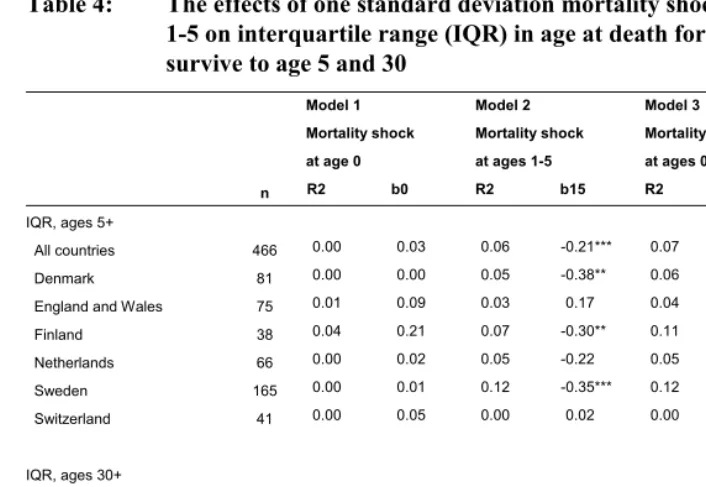
Table 4 shows how compression of mortality, measured by interquartile range in age at death above 5 and 30 years, depends on early life mortality shocks.
Table 4: The effects of one standard deviation mortality shocks at ages 0 and
1-5 on interquartile range (IQR) in age at death for those who survive to age 5 and 30
Model 1 Model 2 Model 3 Mortality shock Mortality shock Mortality shocks at age 0 at ages 1-5 at ages 0 and 1-5
n R2 b0 R2 b15 R2 b0 b15
IQR, ages 5+
All countries 466 0.00 0.03 0.06 -0.21*** 0.07 0.04 -0.21***
Denmark 81 0.00 0.00 0.05 -0.38** 0.06 -0.00 -0.37**
England and Wales 75 0.01 0.09 0.03 0.17 0.04 0.09 0.17
Finland 38 0.04 0.21 0.07 -0.30** 0.11 0.21 -0.30**
Netherlands 66 0.00 0.02 0.05 -0.22 0.05 0.03 -0.22
Sweden 165 0.00 0.01 0.12 -0.35*** 0.12 0.04 -0.35***
Switzerland 41 0.00 0.05 0.00 0.02 0.00 0.05 0.02
IQR, ages 30+
All countries 466 0.00 0.04 0.00 0.03 0.00 0.04 0.03
Denmark 81 0.00 -0.07 0.06 0.24* 0.06 -0.06 0.23*
England and Wales 75 0.01 0.10 0.01 -0.12 0.02 0.10 -0.12
Finland 38 0.00 0.00 0.14 -0.38* 0.14 0.00 -0.38*
Netherlands 66 0.02 0.14 0.00 -0.01 0.02 0.14 0.01
Sweden 165 0.00 0.02 0.01 0.11 0.01 0.01 0.11
Switzerland 41 0.02 -0.13 0.03 -0.17 0.04 -0.12 -0.16
Model 1: b0 is the effect of a 1 SD increase in de-trended cohort mortality at age 0 Model 2: b15 is the effect of a 1 SD increase in de-trended cohort mortality at ages 1-5 Model 3: b0 and b15 are as in Models 1-2, but jointly estimates
2
R
Model 1 of Table 4 analyzes infant mortality shocks. Overall, these shocks explain
very little of the variation in mortality compression (maximum is 0.04), and none of the coefficients is statistically significant.
Model 2 analyzes mortality shocks at ages 1-5. In the pooled regression these
shocks explain 6 % of the variation in mortality compression at ages above 5, but less than 1 % of the variation at ages above 30. Therefore, the effect takes place at ages 5-30. In country-specific regressions and for ages above 5, the coefficients are negative for four countries and highly significant in three countries. England and Wales seems to be an exception here, having a positive (but not significant) coefficient when others are negative. For ages above 30 the effects are a mix of positive and negative coefficients. This confirms that a mortality shock at ages 1-5 has a strong effect on mortality at ages 5-30, but for older ages the effect is weak. The finding is consistent with the findings concerning life expectancy.
The negative association between the shock in child mortality and mortality compression above age 5 means that high childhood mortality compresses later mortality. In Table 4, the estimate -0.21 for the pooled regression implies that one standard deviation shock in mortality at ages 1-5 is associated with 1.6 months’ decrease in interquartile range in age at death (−0.21 0.64 12 1.6⋅ ⋅ = ). Three standard deviation shock in mortality at ages 1-5 then implies a 4.8 months’ decrease in interquartile range in age at death. For Denmark, one standard deviation shock in mortality at ages 1-5 (2.10) decreases variation in age at death by 2.6 months, and the difference between the largest positive (6.20) and largest negative (-5.42) observed shocks would result in 14.3 months’ difference in variation in age at death. For Sweden, these statistics are 3.2 months for one standard deviation shock (2.91) and 21.8 months difference for the difference between the largest (7.47) and smallest (-13.01) observed shocks.
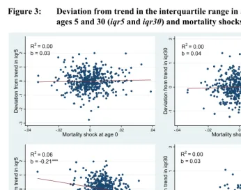
Model 3 estimates jointly the coefficients for infant and early childhood mortality
Figure 3: Deviation from trend in the interquartile range in age at death above
ages 5 and 30 (iqr5 and iqr30) and mortality shocks at ages 0 and 1-5
-3 -2 -1 0 1 2 Devia tio n fr o m tr en d in iq r5
-.04 -.02 0 .02 .04
Mortality shock at age 0
-3 -2 -1 0 1 2 D ev iat io n fr om tr en d i n iq r5
-.015 -.01 -.005 0 .005 .01
Mortality shock at ages 1-4 R2 = 0.00
b = 0.03
R2 = 0.06
b = -0.21***
-1 0 1 2 Devia tion fr o m tr en d in iq r3 0
-.04 -.02 0 .02 .04
Mortality shock at age 0
-1 0 1 2 Devia tion fr o m tr en d in iq r3 0
-.015 -.01 -.005 0 .005 .01
Mortality shock at ages 1-4 R2 = 0.00
b = 0.04
R2 = 0.00
b = 0.03
5.3 Sensitivity analysis
I studied the sensitivity of the results with respect to sex, assumptions regarding the statistical model, time period and mortality level. I first re-estimated the models by sex. The results were similar for both men and women.
Second, I estimated all the models with auto-correlated error structure, allowing the number of lags in the residual to be up to 5. The optimal number of lags was chosen with the generalized Durbin-Watson test. The results were essentially the same with the standard OLS model and with the model that allowed auto-correlation in the residuals.
Third, I estimated the OLS models for the period preceding secular declines in mortality. Among the countries studied, only Sweden has observations for the period preceding mortality decline. The years when mortality was approximately stationary correspond roughly to 1751 to 1810 (1751 being the first year for which data is available, and 1810 being the year after which life expectancy started increasing). The results for Sweden for this time period were consistent with the results reported in Tables 3 and 4.
Fourth, I estimated the OLS models for all countries for the period when life expectancy at birth was below 50. The results were essentially the same as they were for the full data. Additionally, I estimated the models including only the most extreme years. This was done by including a) only the years when infant mortality shock was in the upper 20 % of the distribution, and b) including only the years when deviation from trend in conditional life expectancy between years 5 and 90 was in the upper 20 % of the distribution. Again, the results were similar to what is shown in Tables 3-4.
Finally, the models were re-estimated with log-mortality as the basis of cohort mortality shocks (instead of using mortality on original scale). The results did not change in any significant way.
6. Discussion
not particularly strongly. The strongest effects were observed for England and Wales where the long-term decrease in infant mortality from the mid-19th century to early 20th century was associated with a 1.5 year increase in life expectancy at age 5. This effect is approximately 10% of the long term increase in life expectancy at age 5. For other countries, however, the effects were markedly smaller and statistically insignificant. The effects for older ages were also small.
There was no evidence that compression of mortality would depend on shocks in infant mortality. Mortality shocks at ages 1-5, however, were strongly linked to mortality at ages 5-30 and variation in age at death at ages above 5. High early childhood mortality increases average number of years lived for those who survive to age 5 and compresses mortality. High mortality at ages 1-5 may also slightly decrease conditional life expectancy at old ages, but the evidence for this is weak both substantively and statistically. These findings were similar for men and women.
The finding that high mortality at ages 1-5 may decrease mortality at ages 5-30 may be due to selection or acquired immunity during the mortality shock. For all cohorts, mortality is very low at ages 5-30. Thus those few who die at these ages are likely to be very frail (wartimes, and accident mortality, may constitute exceptions). If mortality at ages 1-5 happens to be higher than on average, then it is plausible that this mortality shock especially affects those who would otherwise have lived to age 5 but who still died at relatively young ages. If this is true, the selection and culling effect would explain the observed association between mortality at ages 1-5 and 5-30. The other explanation, acquired immunity during the shock, is also possible, but in this study it was not possible to separate these two explanations.
cohort mortality patterns have been well documented (Winter 1976). Derrick (1927; cited in Winter 1976) even claimed that, “[in England and Wales] the effects of losses during the European War were so great and indefinite as to obscure all normal changes”. Of course, the mortality dynamics may also be inherently different in England and Wales than they are in other countries. Even if it were true, the overall evidence from pooled regressions and from other countries still suggests that above-trend mortality from the ages of 1-5 decreases mortality at older ages up to age 20-30. The reasons why the link between infant mortality and life expectancy at ages 5-90 is stronger in England and Wales than in other countries, however, remains unclear.
This study did not find any strong gender differences in how mortality depends on early life cohort and later life period shocks. Theories which would predict that one of the sexes should be more robust to harmful early life conditions are plentiful (Crimmins and Finch 2006a), but they are not consistent with each other. In previous research Catalano and Bruckner (2006) and van den Berg et al. (2007) found some indication that women are more robust than men, but Crimmins and Finch (2006a) obtained the opposite result. Others have found no or only small differences (van den Berg, Lindeboom and Portrait 2006; van den Berg et al. 2008). As the empirical evidence is so inconsistent, a tentative conclusion is that there are no strong differences between the two sexes.
The results of this study – no marked increase in old-age mortality for cohorts who had higher than expected infant and early childhood mortality – are consistent with the studies finding no increased mortality for those who survived great famines as young children (Kannisto, Christensen, and Vaupel 1997; Painter et al. 2005) or who were exposed to disease in utero or soon after birth (Cohen and Tillinghast 2009). The findings are also consistent with the emerging literature suggesting that cohort’s old-age mortality depends weakly at best on cohort’s early life mortality (Bruckner and Catalano 2009; Gagnon and Mazan 2009; van den Berg et al. 2009). While mortality is unlikely to capture all relevant dimensions of early life conditions, it is likely that cohort-to-cohort infant and child mortality reflects some of the potentially most important early life cohort-level factors such as nutritional status and exposure to disease. All in all, however, the weak links between cohort-level early and later mortality suggest that old-age mortality may depend more on later life period conditions than early life conditions.
and Dutch cohorts which were the subjects of these studies. Cutler et al. (Cutler, Miller and Norton 2007), however, who focus on the effect of the 1930s great depression, do not find any health effects for later life. It may be that the link between macroeconomic conditions early in life and later health and mortality are not as strong in the 20th century (and 21st century) as they were historically. An important future research question is what are mechanisms and pathways that link macroeconomic conditions at the time of birth to later health, and how relevant are these mechanisms in contemporary developing and developed world.
7. Acknowledgements
References
Almond, D. (2006). Is the 1918 Influenza Pandemic Over? Long-Term Effects of In Utero Influenza Exposure in the Post-1940 U.S. Population. Journal of Political Economy 114(4): 672-712. doi:10.1086/507154.
Andreev, K. (2002). Evolution of the Danish Population from 1835 to 2000. Odense: Odense University Press.
Barbi, E. and Vaupel, J.W. (2005). Comment on "Inflammatory exposure and historical changes in human life-spans". Science 308(5729): 1743.
Barker, D.J., Eriksson, J.G., Forsen, T., and Osmond, C. (2002). Fetal origins of adult disease: strength of effects and biological basis. International Journal for Epidemiology 31(6): 1235-1239. doi:10.1093/ije/31.6.1235.
Barker, D.J.P. (1992). Fetal and Infant Origins of Adult Disease. London, UK: British Medical Journal Publishing.
Barker, D.J.P. (1994). Mothers, Babies, and Disease in Later Life. London, UK: British Medical Journal Publishing.
Bengtsson, T.and Lindstrom, M. (2000). Childhood misery and disease in later life: the effects on mortality in old age of hazards experienced in early life, southern Sweden, 1760-1894. Population Studies (Cambrigde) 54(3): 263-277.
doi:10.1080/713779096.
Bengtsson, T.and Lindstrom, M. (2003). Airborne infectious diseases during infancy and mortality in later life in southern Sweden, 1766-1894. International Journal for Epidemiology 32(2): 286-294. doi:10.1093/ije/dyg061.
Bengtsson, T. and Broström, G. (2009). Do conditions in early life affect old-age mortality directly and indirectly? Evidence from 19th-century rural Sweden.
Social Science & Medicine 68(9): 1583-1590.
doi:10.1016/j.socscimed.2009.02.020.
Bengtsson, T. and Mineau, G.P. (2009). Early-life effects on socio-economic performance and mortality in later life: A full life-course approach using contemporary and historical sources. Social Science & Medicine 68(9): 1561-1564. doi:10.1016/j.socscimed.2009.02.012.
Bruckner, T.A. and Catalano, R.A. (2009). Infant mortality and diminished entelechy in three European countries. Social Science & Medicine 68(9): 1617-1624.
Case, A., Fertig, A., and Paxson, C. (2005). The Lasting Impact of Childhood Health and Circumstance. Journal of Health Economics 24(2): 365-389.
doi:10.1016/j.jhealeco.2004.09.008.
Catalano, R. and Bruckner, T. (2006). Child mortality and cohort lifespan: a test of diminished entelechy. International Journal for Epidemiology 35(5): 1264-1269.
doi:10.1093/ije/dyl108.
Cohen, A.A. and Tillinghast, J. (2009). No consistent effects of prenatal or neonatal exposure to Spanish flu on late-life mortality in 24 developed countries. In: Population Association of America. Annual Meeting Detroit, MI.
Costa, D.L. and Lahey, J.N. (2005). Predicting older age mortality trends. Journal of the European Economic Association 3(2-3): 487-493. doi:10.1162/jeea.2005.3.2-3.487.
Crimmins, E.M. and Finch, C.E. (2006a). Commentary: Do older men and women gain equally from improving childhood conditions? International Journal for Epidemiology 35(5): 1270-1271. doi:10.1093/ije/dyl194.
Crimmins, E.M. and Finch, C.E. (2006b). Infection, inflammation, height, and longevity. Proceedings of the National Academy of Science 103(2): 498-503.
doi:10.1073/pnas.0501470103.
Cutler, D.M., Miller, G., and Norton, D.M. (2007). Evidence on early-life income and late-life health from America's Dust Bowl era. Proceedings of the National Academy of Sciences 104: 13244-13249. doi:10.1073/pnas.0700035104.
Derrick, V.P.A. (1927). Observations on (1) errors in age in the population statistics of England and Wales, and (2) the changes in mortality indicated by the national records. Journal of the Institute of Actuaries 58: 117-159.
Doblhammer, G. (2004). The Late Life Legacy Very Early Life. Springer Verlag. Edwards, R. and Tuljapurkar, S. (2005). Inequality in life spans and a new perspective
on mortality convergence across industrialized countries. Population and Development Review 31: 645-675. doi:10.1111/j.1728-4457.2005.00092.x
Eriksson, J.G., Forsen, T., Tuomilehto, J., Winter, P.D., Osmond, C., and Barker, D.J. (1999). Catch-up growth in childhood and death from coronary heart disease: longitudinal study. British Medical Journal 318(7181): 427-431.
Finch, C.E. and Crimmins, E.M. (2004). Inflammatory exposure and historical changes in human life-spans. Science 305(5691): 1736-1739.
Fogel, R.W. (2004). The Escape from Hunger and Premature Death, 1700-2100: Europe, America, and the Third World. New York: Cambridge University Press. Fries, J.F. (1980). Aging, natural death, and the compression of morbidity. New
England Journal of Medicine 303: 130-135.
Gagnon, A. and Mazan, R. (2009). Does exposure to infectious diseases in infancy affect old-age mortality? Evidence from a pre-industrial population. Social Science & Medicine 68(9): 1609-1616. doi:10.1016/j.socscimed.2009.02.008. Hayward, M.D. and Gorman, B.K. (2004). The long arm of childhood: The influence of
early-life social conditions on men's mortality. Demography 41: 87-107.
doi:10.1353/dem.2004.0005.
Hendry, D.F. (1980). Econometrics-Alchemy or Science? Economica 47(188): 387-406. doi:10.2307/2553385.
Hodrick, R.J. and Prescott, E.C. (1997). Postwar U.S. Business Cycles: An Empirical Investigation. Journal of Money, Credit and Banking 29(1): 1-16.
doi:10.2307/2953682.
Human Mortality Database, University of California, Berkeley (USA), and Max Planck Institute for Demographic Research (Germany). Available at www.mortality.org or www.humanmortality.de (data downloaded on January 10 2008).
Jdanov, D., Scholz, R., and Shkolnikov, V.M. (2005). Official population statistics and the Human Mortality Database estimates of populations aged 80+ in Germany and nine other European countries. MPIDR Working Paper 2005-010.
Kannisto, V. (2000). Measuring the Compression of Mortality. Demographic Research 3(6). doi:10.4054/DemRes.2000.3.6.
Kermack, W.O., McKendrick, A.G., and McKinlay, P.L. (1934). Death rates in Great Britain and Sweden: Some general regularities and their significance. Lancet 226: 698-703. doi:10.1016/S0140-6736(00)92530-3.
Kermack, W.O., McKendrick, A.G., and McKinlay, P.L. (2001). Death-rates in Great Britain and Sweden. Some general regularities and their significance.
International Journal for Epidemiology 30(4): 678-683.
doi:10.1093/ije/30.4.678.
Lee, C. (1997). Socioeconomic Background, Disease, and Mortality Among Union Army Recruits: Implications for Economic and Demographic History. Explorations in Economic History 34(1): 27-55. doi:10.1006/exeh.1996.0661. Maravall, A. and del Río, A. (2007). Temporal aggregation, systematic sampling, and
the Hodrick-Prescott filter. Bank of Spain Documents de Trabajo, Madrid. Painter, R.C., Roseboom, T.J., Bossuyt, P.M., Osmond, C., Barker, D.J., and Bleker,
O.P. (2005). Adult mortality at age 57 after prenatal exposure to the Dutch famine. European Journal for Epidemiology 20(8): 673-676.
doi:10.1007/s10654-005-7921-0.
Preston, S.H., Hill, M.E., and Drevenstedt, G.L. (1998). Childhood conditions that predict survival to advanced ages among African-Americans. Society, Science & Medicine 47(9): 1231-1246. doi:10.1016/S0277-9536(98)00180-4.
Ravn, M.O. and Uhlig, H. (2002). On Adjusting the Hodrick-Prescott Filter for the Frequency of Observations. The Review of Economics and Statistics 84(2): 371-376. doi:10.1162/003465302317411604.
Van den Berg, G.J., Lindeboom, M., and Portrait, F. (2006). Economic Conditions Early in Life and Individual Mortality. American Economic Review 96(1): 290-302. doi:10.1257/000282806776157740.
Van den Berg, G.J., Doblhammer-Reiter, G., and Christensen, K. (2008). Being Born Under Adverse Economic Conditions Leads to a Higher Cardiovascular Mortality Rate Later in Life: Evidence Based on Individuals Born at Different Stages of the Business Cycle. IZA Discussion Paper No. 3635.
Van den Berg, G.J., Lindeboom, M., and Portrait, F. (2007). Long-Run Longevity Effects of a Nutritional Shock Early in Life: The Dutch Potato Famine of 1846-1847. IZA Discussion Paper No. 3123
Wilmoth, J., Vallin, J., and Caselli, G. (1990). When Does a Cohort's Mortality Differ from What we Might Expect? Population: An English Selection 2: 93-126. Wilmoth, J.R. and Horiuchi, S. (1999). Rectangularization revisited: variability of age
at death within human populations. Demography 36(4): 475-495.
doi:10.2307/2648085.