University of New Orleans Theses and
Dissertations Dissertations and Theses
8-7-2008
Clustering Via Supervised Support Vector Machines
Clustering Via Supervised Support Vector Machines
Sepehr Merat
University of New Orleans
Follow this and additional works at: https://scholarworks.uno.edu/td
Recommended Citation Recommended Citation
Merat, Sepehr, "Clustering Via Supervised Support Vector Machines" (2008). University of New Orleans Theses and Dissertations. 857.
https://scholarworks.uno.edu/td/857
A Thesis
Submitted to the Graduate Faculty of the University of New Orleans
in partial fulfillment of the requirements for the degree of
Master of Science in
Computer Science
by Sepehr Merat
B.Sc. Simon Fraser University, 2006
I deeply thank my dear advisor Dr. Winters-Hilt for all of his help and support. He also taught me the importance of common sense, simplicity and maturity in research, work and life in general.
Acknowledgment iv
Abstract xi
1 Introduction 1
1.1 Motivation . . . 1
1.2 Overview . . . 2
2 Introduction to Classification 3 2.1 Theory of Classification . . . 3
2.2 Kernel Feature Spaces . . . 6
2.3 Reproducing Kernel Hilbert Spaces – RKHS . . . 8
2.4 Component Analysis . . . 11
2.4.1 Principal Component Analysis – PCA . . . 11
2.4.2 Kernel Principal Component Analysis – KPCA . . . 13
2.5 Supervised Learning . . . 16
2.5.1 Margins . . . 16
2.5.2 Support Vector Machines . . . 17
2.6 Unsupervised Learning (Clustering) . . . 22
2.6.1 K-means . . . 22
2.6.2 Kernel K-means . . . 23
3.2 Kernel Construction Using Polarization . . . 33
3.2.1 “Occam’s Razor” Kernels . . . 33
3.2.2 Regularized Distance Kernels . . . 34
3.2.3 Regularized Divergence Kernels . . . 35
3.3 Supervised Cluster Validators . . . 37
3.3.1 Purity. . . 39
3.4 Unsupervised Cluster Validator . . . 40
3.4.1 Kernel-Sum-of-Squared-Error (Kernel SSE) . . . 40
3.5 SVM-Relabeler Clustering Method . . . 42
3.6 Refinement Methods Using Simulated Annealing . . . 44
4 SVM-Relabeler Results 47 4.1 Iris Data Set . . . 47
4.2 DNA Hairpin Data Set . . . 55
5 Conclusion 64 5.1 Discussions and Future Work . . . 64
5.1.1 Regularized Divergence Kernels . . . 64
5.1.2 Cluster Validators . . . 65
5.1.3 Tuning of SVM-Relabeler . . . 66
5.2 Concluding Remarks . . . 67
Bibliography 68 A Proof of Non-Positive-Definitivity of the Sentropic Kernel 72 B kernlib Framework 75 B.1 Configuration . . . 75
B.2 SVM engine . . . 75
2.1 This figure illustrates relation (2.3). In practice the goal is to find the best trade-off between empirical error and the complexity. This figure is based on the illusteration in [4] . . . 5
3.1 Confusion matrix for a 2-class problem . . . 37
3.2 SVM on non-separable features . . . 42
3.3 (a) demonstrates the histogram and the fitted distribution by randomly labeling the 8GC/9GC data set using the Absdiff kernel (γ = 1.8) and computing SSE. The fitted Distribution is Johnson’s SB distribution
(see Appendix) (γ = −5.5405, δ = 1.8197, λ = 2.7483, ξ = 168.46) with the corresponding Q-Q plot in (b). . . 46
4.1 SVM-Relabeler using a polynomial kernel . . . 48
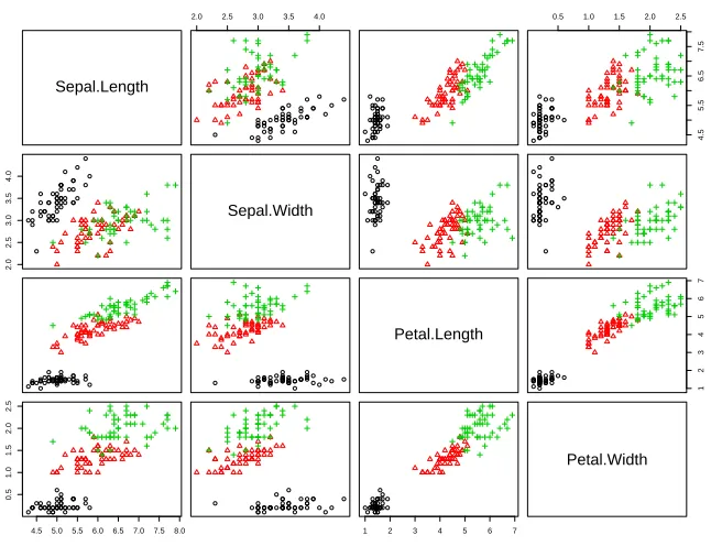
4.2 Iris data set: black circles represent setosa, red triangles represent versicolor, and green pluses represent virginica. . . 48
4.3 3 different trials of SVM-Relabeler algorithm demonstrating the range of the possible solution space as measured by SSE ((a), Absdiff kernel
γ = 1.8) and purity ((b), see appendix)) . . . 56 4.4 This figure shows the progress of the SVM-Relabeler algorithm as it
figure that by iteration 17 the data set has been clearly separated. Figure (b) shows, iteration by iteration for the same experiment as in (a), a decrease in Kernel SSE value, test and training errors and
simultanous increase in the purity. . . 61
4.6 This figure compares the behavior of Algorithm 9 using constant and variable perturbation functions. Top-left demonstrates the case where constant 10% perturbation is applied at every iteration, while in ad-dition to that, the top-right figure increases the probability of pertur-bation based on the number of iterations during which SSE remained constant (bottom-right). The bottom-left figure shows the annealing process. . . 63
B.1 Example property file to configure data, train and test using an SMO SVM engine, and cluster using the SVM-Relabeler engine . . . 76
B.2 Example java class mapping file. . . 77
B.3 Simple initialization of the SVM engine. . . 77
B.4 Learning using the SVM engine. . . 78
B.5 Prediction using the SVM engine. . . 78
An SVM-based clustering algorithm is introduced that clusters data with no a priori knowledge of input classes. The algorithm initializes by first running a binary SVM classifier against a data set with each vector in the set randomly labeled. Once this initialization step is complete, the SVM confidence parameters for classification on each of the training instances can be accessed. The lowest confidence data (e.g., the worst of the mislabeled data) then has its labels switched to the other class label. The SVM is then re-run on the data set (with partly re-labeled data). The repetition of the above process improves the separability until there is no misclassification. Variations on this type of clustering approach are shown.
Keywords: clustering, machine learning, pattern recognition, support vector
Introduction
1.1
Motivation
The goal of clustering analysis is to partition objects into groups, such that the members of each group are more “similar” to each other than the members of other groups. The similarity is determined subjectively as it does not have a universally agreeable upon definition. In [1] the author suggests a formal perspective on the difficulty in finding such a unification, in the form of an impossibility theorem: for a set of three simple properties, there is no clustering function satisfying all three. Furthermore, the author demonstrates that relaxations of these properties expose some of the interesting (and unavoidable) trade-offs at work in well-studied clustering techniques such as single-linkage, sum-of-pairs, k-means, and k-median.
1.2
Overview
Introduction to Classification
2.1
Theory of Classification
The problem of classification is to find a general rule, that based on a set of given observations a machine is trained to match a set of objects to their appropriate classes. In its simplest form the machine’s task is to estimate a function f : RN → {±1},
using a set of independent and identically distributed training data set according to an unknown probability distribution P(x, y), such that if future example pairs (x, y) are drawn from the same probability distributionP(x, y),f would be able to perfectly classify them as +1 if f(x) ≥0 or -1 if otherwise. To clarity, each example is a pair that includes a vector of features (or observations), x, and a corresponding label (or response), y. In the case of the above binary classification the examples are in fact:
(x1, y1), . . . ,(xn, yn)∈RN ×Y, Y ={±1}
The best function, f, is theoretically obtained by minimizing the expected risk func-tion (expected error) (cf. [3]):
R[f] = Z
where l is a suitable loss function. For instance, in the case of’ “0/1 loss”
l(f(x), y) = Θ(−yf(x))
where Θ is the Heaviside function (Θ(z) = 0 for z < 0 and Θ(z) = 1 otherwise.) In most realistic cases P(x, y) is unknown and therefore the risk function above cannot be used to find the optimum functionf. To overcome this fundamental limitation one has to use the informationhidden in the limited training examples and the properties of the function class F to approximate this function. Hence instead of minimizing the expected risk in (2.1), one may minimize the empirical risk
Remp[f] = 1/n n
X
i=1
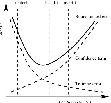
l(f(xi), y). (2.2) As a by product, the learning machine can ensure that for n → ∞ the emper-ical risk will asymptotemper-ically converge to expected risk, but for a small training set the resulting deviations are often large. This leads to a phenomenon called “over-fitting.” Then a small generalization error cannot be obtained by simply minimizing the training error (2.2). One way to avoid the over-fitting dilemma is to restrict the complexity of the function class that one chooses the function from [4]. The intuition, which will be formalized in the following is that a “simple” (e.g., linear) function that explains most of the data is preferable to a complex one (Occams razor). Typically one introduces a regularization term to limit the complexity of the function class from which the learning machine can choose. This way the model selection – finding an optimal complexity of the function – is necessary (cf. [5]).
A specific way of controlling the complexity of a function class is given by the Vapnik-Chervonenkis (VC) theory and the structural risk minimization (SRM) prin-ciple [4], [6]. Here the concept of complexity is captured by the VC dimensionhof the function class F that the estimate f is chosen from. The following set of definition clarify the rest of this discussion.
Error
VC dimension (h)
Confidence term
Training error Bound on test error overfit
best fit underfit
Figure 2.1: This figure illustrates relation (2.3). In practice the goal is to find the best trade-off between empirical error and the complexity. This figure is based on the illusteration in [4]
if and only if for every possible training set of the form (x1, y1), . . . ,(xn, yn)there
ex-ists some parameter set α that gets zero training error (empirical risk).
Definition 2 (VC Dimension) Given a learning machine f, the VC-dimension h
is the maximum number of points that can be arranged so that f shatter them.
Roughly speaking, the VC dimension measures how many (training) points can be shattered (i.e., separated) for all possible labelings using functions of the class. Constructing a nested family of function classes F1 ⊂ . . . ⊂ Fk with nondecreasing
VC dimension the SRM principle proceeds as follows:
Definition 3 (SRM Principle) Letf1, . . . , fk be the solutions of the empirical risk
minimization (2.2) in the function classesFi. SRM chooses the function classFi (and
the function fi ) such that an upper bound on the generalization error is minimized
which can be computed making use of theorems such as the following one (see Figure (2.1)).
Theorem 4 (Expected Risk Upperbound) Let h denote the VC dimension of
delta >0 and f ∈F the inequality bounding the risk
R[f]≤Remp[f] +
s
h(ln2n
h + 1)−ln
δ
4
n (2.3)
holds with probability of at least 1−δ for n > h .([4], [6])
Note, this bound is only an example and similar formulations are available for other loss functions (cf. [6]) and other complexity measures, e.g., entropy numbers [7]. In the equation (2.3): the goal is to minimize the generalization errorR[f], which can be achieved by obtaining a small training errorRemp[f] while keeping the function
class as small as possible. Two extremes can arise for equation (2.3): i) a very small function class (like F1 ) yields a vanishing square root term, but a large training error might remain, while ii) a huge function class (likeFk) may give a vanishing empirical
error but a large square root term. The best class is usually in between (see Figure (2.1)), as one would like to obtain a function that explains the data quite well and to have a small risk in obtaining that function. This is very much in analogy to the bias-variance dilemma scenario described for neural networks (see, e.g., [8]).
2.2
Kernel Feature Spaces
The so-calledcurse of dimensionality from statistics says essentially that the difficulty of an estimation problem increases drastically with the dimension N of the space, since in principle as N increases, the number of required patterns to sample grows exponentially. This statement casts doubts in using high dimensional feature vectors as input to learning machines. Fortunately, results from statistical learning theory [4] also show that the likelihood of data separability by linear learning machines is proportional to its dimensionality.
Therefore, instead of working in the RN, one can design algorithms to work in feature space, F, where the data has much higher dimension. This can be done via the following mapping
In (2.4) the data x1, . . . ,xn ∈ RN is mapped into a potentially much higher dimen-sional feature space F. For a given learning algorithm one now considers the same algorithm in F instead of RN. Hence, the learning machine works with the following sample:
(Φ(x1), y1), . . . ,(Φ(xn), yn)∈ F ×Y, Y ={±1}
It is important to note that this mapping is also implicitly done for (one hidden layer) neural networks, radial basis networks (cf. [9]) and boosting algorithms (cf. [10]) where the input data is mapped to some representation given by the hidden layer, the radial basis function (RBF) bumps or the hypotheses space, respectively.
As a consequence of the above discussion, the dimensionality of the data does not detract us from finding a good solution, but it is rather the complexity of the function class F that contributes the most to the complexity of the problem at hand. Similarly, in practice one would never need to know the mapping function Φ, and therefore the complexity and intractability of computing the actual mapping is also irrelevant to the complexity of the problem of classification. To this end, algorithms are transformed to take advantage of a method called the Kernel Trick.
Definition 5 (Kernel Trick) Achieve the following two objectives when using a
learning machine:
1) Rewrite our learning algorithm so that instead of using Φ(x1) and Φ(x2) directly,
it only uses the dot-product K(x1,x2) = Φ(x1)·Φ(x2), and
2) Compute the dot-products K(x1,x2) in a manner, that avoids computing Φ(x1)
and Φ(x2) explicitly.
Kernel trick in definition (5) requires the knowledge of the appropriateness of a given function, K, to be used as a kernel. Mercer’s Condition is a way to test for admission, and is stated in the following theorem.
Theorem 6 [Mercer’s Condition][3] For a given function, K, there exists a mapping
Φ and an expansion:
K(x,y) = X
i
if and only if, for any function, g(x) such that
Z
g(x)2dx
is finite, then
Z Z
K(x,y)g(x)g(y)dxdy≥0
Note, that it is usually difficult to apply Theorem (6) directly, since the final integra-tion is hard to perform for complex candidate kernel funcintegra-tions.
To summarize, any linear classifier that can be formulated to avoid explicit cal-culation of the mapping function Φ, could be used to classify nonlinear data. The argument advanced in the next section expands upon the theory of admissible kernels.
2.3
Reproducing Kernel Hilbert Spaces – RKHS
In section (2.2) the notions of Kernel and higher dimension maps were introduced. Basically, kernels can be used to convert some linear learning algorithms to non-linear algorithms, without concerning us with the actual mapping. Admission of functions to be kernels depends on the disscussion that follows in this section. Formally put,
Definition 7 Kernel is any symmetric function K : χ×χ→ R. Kernel is said to
be:
(i) Positive Definite if P
K(xi, xj)cicj ≥0
(ii) Negative Definite if P
K(xi, xj)cicj ≤0, such that Pci = 0
Consider the Hilbert space1 L
2 : hu, wi = R
u(t)v(t)dt. L2 contains too many non-smooth functions and Reproducing Hilbert Kernel Spaces provides us with the restriction necessary to obtain a smaller well behaved Hilbert space. Given a kernel
K(x, x′), the goal is to construct a Hilbert space in which K is a dot product. That
is,
Definition 8 A kernel, K, on set χ is pd iff ∃ a Hilbert space, H, and a map Φ :
χ→H such that ∀x, y ∈χ,
K(x, y) =hΦ(x),Φ(y)i Further define the following reproducing kernel map:
φ:x7→K(·, x)
that is, to each vector x in the input space χ we assign a function K(·, x). We can now construct RKHS, a vector space from the linear combinations of the range of the above map,
f(·) =X
i
αiK(·, xi).
The inner product of f(·) and g(·) for g(·) = P
jβjK(·, x′j) is then defined as:
hf, gi=X
i
X
j
αiβjK(xi, x′j). (2.5)
1A Hilbert space is a vector spaceHover a topological field (eitherRorC) with an inner product
h·,·i. That is given vectorsu, v, andw∈ Hand scalarsλandµ,
hλu+µv, wi = λhu, wi+µhv, wi hu, vi = hv, ui
hu, ui ≥ 0
hu, ui= 0 → x= 0
From h·,·i we get a norm || · || via ||u|| = p
hu, ui. This norm allows us to define notions of
Note that for any given f(·) as defined above,
hK(·, x), fi=X
i
αiK(xi, x) =f(x)
shows that the kernel, k, is the representer of evaluation. Finally,
2.4
Component Analysis
2.4.1
Principal Component Analysis – PCA
The goal of PCA is to find a new set of dimensions that better capture the variabil-ity of the data. In fact, the amount of variabilvariabil-ity captured by the new dimensions decreases with higher dimensions. That is the first dimension captures most of the variability; the second dimension is orthogonal to the first and captures as much vari-ability as allowed by providing that constraint and so on. In a more mathematical way, PCA’s tenet is to compute the most meaningful basis to re-express a noisy data set. The hope is that this new basis will filter out the noise an reveal the hidden structure. If the data is represented using a matrix with columns being the like at-tributes, PCA results in the following set of properties:
1- The covariance of each new two columns is zero.
2- Columns are ordered with respect to the amount of variability they captured. 3- First column contains as much and most of the variability of the data,
4- Subject to the constraint of orthogonality, each subsequent column contains as much variability as possible.
Futhermore, PCA contains the following assumptions: 1- Linearity,
2- Mean and variance are sufficient statistics2, 3- Large variance is of structural importance, and 4- The principal components are orthogonal.
Supposing that the data matrix, X, is centered – meaning that the mean of each column is 0. Our objective is to find transformation matrix P such that the new
2A statisticS(X) is sufficient for underlying parameterαif the conditional probability
distribu-tion of the input dataX, given the statisticS(X), is independant of the parameter,α. Formally,
P r(X=x|S(X) =s, α) =P r(X =x|S(X) =s). (2.6)
matrix Y can be written as:
Y =P X
where the rows of P are the principal components of X. Since it is desired that the columns are Y have zerocovariance, the covariance matrix of Y should have all zeros on its off diagonals. Therefore, the covariance matrixC = n−11Y YT needs to be
diagonalized. With a substitution A=XXT we can rewrite C as:
C= 1
n−1P(XX
T)T PT = 1
n−1P AP
T (2.7)
NoteA is symmetric it must be orthogonally diagonalizable. since:
AT = (EDET)T =ET TDTET =EDET =A (2.8) In PCA the trick is thatP is chosen so that each row ofP is an eigenvector ofA and therefore,XXT. Combining with (2.7), (2.8),
C = 1
n−1P AP
T = 1
n−1D (2.9)
It is shown that P diagonalizes C and therefore the rows ofP, principal components of X are eigenvectors ofXXT. Algorithm (1) demonstrates PCA procedure.
Algorithm 1 PCA Procedure
Require: data set X
1: Subtract the mean for each column of X
2: Calculate the covariance matrix S
3: Find the eigenvectors, P, and the eigenvalues,v of XXT 4: Sort P rows based on v’s values
2.4.2
Kernel Principal Component Analysis – KPCA
Derivation
Kernel PCA uses the kernel trick in section (2.2) to relax the linearity assumption in the regular PCA. There for KPCA is a generalization PCA to the case where we are not interested in principal components in input space, but rather in principal components of features which are non-linearly related to the input features. This amounts to taking higer-order correlations between input features.
Recall that the input space covariance matrix SI = 1/(n−1)XXT can be written
as SI = 1/(n−1)Pnj=1xjxTj, where X is centered input feature matrix. In feature
space this can be modified to:
S≡SF = 1/(n−1) n
X
j=1
Φ(xj)Φ(xj)T.
Also recall that the principal components are calculated via:
λP =SP = 1
n−1
n
X
j=1
(Φ(xj)·P)Φ(xj). (2.10) It can be seen from (2.10) thatP ∈span{Φ(x1), . . .Φ(xn)} and therefore,
P =
n
X
j=1
αjΦ(xj). (2.11)
by multiplying Φ(xk) by λP in (2.10) we obtain:
λ(Φ(xk)·P) = Φ(xk)·SP (2.12) Furthermore, by combining (2.10) and (2.12) we obtain
λ
n
X
j=1
αj(Φ(xk)·Φ(xj)) =
1
n−1
n
X
j=1
αj(Φ(xk) n
X
i=1
Φ(xi))(Φ(xj)·Φ(xi)) (2.13)
As before let Kij be ann×n matrix defined by:
Kij = Φ(xi)·Φ(xj). (2.14)
Equation (2.13) is therefore simplified to:
(n−1)λα=Kα (2.15) The matrix K is positive semi-definite and hence the eigenvalues are all positive. First we sort eigenvalues using λ1 ≤ . . . ≤ λn with corresponding eigenvectors as
α1, . . . ,αn. Then we normalize α1, . . . ,αn by requiring that the corresponding vec-tors in F be normalized such that Pk·Pk = 1 for all k ∈ {index of non-zero
eigen-values}. This condition can be derived from (2.10) and (2.10) by requiring that
1 = λk(αk·αk) (2.16)
Finally, to extract features of a new observationxone can project the mapped pattern Φ(x) onto Pk using
Pk·Φ(x) =
n
X
j=1
αkj(Φ(xj)·Φ(x)) =
n
X
j=1
αkjk(xj,x). (2.17)
Implementation
So far we assumed that the mapped data is centered in F. That is:
n
X
j=1
We do not have to assume this since
˜
Φ(xi)≡Φ(xi)−1/n
n
X
j=1
Φ(xj) (2.19)
is centered for any given set of features xj, for all j between 1 to n. Therefore the previous analysis holds if we replace all Φ with ˜Φ. We can also write ˜K in terms of
K which results in: ˜
Kij = ˜Φ(xi)TΦ(˜ xj)
= (Φ(xi)−1/n
n
X
k=1
Φ(xk))T(Φ(xj)−1/n
n
X
k=1
Φ(xk))
= Φ(xi)TΦ(xj)−1/n
n
X
k=1
Φ(xk)TΦ(xj)−1/n
n
X
k=1
Φ(xi)TΦ(xk)
+1/n2
n
X
k,k′=1
Φ(xk)TΦ(xk′)
By letting (1n)ij ≡1/n, we can rewrite the above as:
˜
Kij =K−1nK−K1n+ 1nK1n. (2.20)
This modification does not affect the formulation as long as K is replaced with equa-tion (2.20). This process is demonstrated in algorithm (2).
Algorithm 2 KPCA Procedure
Require: data set X
Require: Feature vector x
1: Calculate kernel matrix K
2: Calculate ˜K from (2.20)
3: Diagonalize ˜k using the eigenvalue decomposition in (2.10)
2.5
Supervised Learning
2.5.1
Margins
As justified in section (2.2) we can assume that the training sample is separable by a hyperplane, and therefore the following learning machine.
f(x) = (ω·x)−b (2.21) In [4] it is shown that the for this class of hyperplanes the VC dimension can be bounded in terms of another quantity, the margin. The margin is defined as the minimal distance of a sample to the decision surface (see section 2.5.2). It is rather intuitive that the thicker the margin the better the training would be, and in fact this quantity could be measured by the length of the weight vector, ω in (2.21). since we assumed that the training data is separable we can rescale and normalize
ω such that the points closest to the hyperplane is a unit away from the hyperplane (i.e., the canonical representation of the hyperplane). This can be done by requiring that |(ω·x)−b)| = 1. Now consider two samples x1 and x2 from different classes with (ω · x1) −b = 1 and (ω ·x2)− b = −1, respectively. The margin is given by the distance of these two points, measured perpendicular to the hyperplane and therefore, ω/||ω||2·(x1−x2) = 2/||ω||2. The concept of margins links this intuitive result to another result from VC dimension of linear hyperplanes [4]. In fact, using the notation from [4] and Theorem (9), we can control its VC dimension if we bound the function class to be below 2/Λ.
Theorem 9 [4] For the class of separating hyperplane with margin ||ω||2 the
inequal-ity:
h≤Λ2R2+ 1 (2.22)
and
||ω||2≤Λ (2.23)
2.5.2
Support Vector Machines
In this section we treat a supervised separating hyperplane learning machine, called Support Vector Machines (SVMs), which incorporate the results in section (2.5.1). As a consequence SVMs are less susceptible to over-fit even with a poor choice of kernel and parameters. The rest of this section focuses on the specifics of derivation and implementation of such learners.
Derivation
Using the convention of implied sum on repeated Greek indices, throughout the rest of this derivation, feature vectors are denoted by xik, where indexilabels the feature
vectors (1≤i≤M) and indexklabels theN feature vector components (1≤k≤N). Similarly, labeling of training data is done using label variable yi = ±1 (with sign
according to whether the training instance was from the positive or negative class). For hyperplane separability, elements of the training set must satisfy the following conditions: ωβxiβ −b = +1 fori such thatyi = +1, andωβxiβ−b=−1 foryi =−1,
for some values of the weight coefficientsω1, . . . , ωN, and b. This can be written more
concisely as: yi(ωβxiβ−b)−1 = 0. Data points that satisfy the equality in the above
are known as “support vectors” (or ”active constraints”).
Once training is complete, discrimination is based solely on position relative to the discriminating hyperplane: ωβxiβ −b = 0. The boundary hyperplanes on the
two classes of data are separated by a distance 2/||ω||2, known as the ”margin” (section 2.5.1), where||ω||2
2 =ωβωβ. Note that by increasing the margin between the
separated data as much as possible the optimal separating hyperplane is obtained. Furthermore, the goal to maximize ||ω||−21 can be restated as the goal to minimize
||ω||2
2. The Lagrangian variational formulation then selects an optimum defined at a saddle point of
L(ω, b;α) = ωβωβ
2 −αγyγ(ωβxγβ−b)−α0 (2.24) Subject to: α0 =
X
γ
Therefore, the saddle point is obtained by minimizing with respect to
{ω1, . . . , ωNb} and maximizing with respect to {α1, . . . , αM}.
Now, if yi(wβxiβ −b)−1 ≥ 0, then maximization on αi is achieved for αi = 0.
On the other hand, if yi(wβxiβ −b)−1 = 0, then there is no constraint on αi and
if yi(wβxiβ −b)−1 < 0, there is a constraint violation, and αi → ∞. In the case
of absolute separability, the last case will eventually be eliminated for all αi. But if
separability is not possible it is natural to limit the size ofαi by some constant upper
bound, i.e., max(αi) = C, for all i. This is equivalent to another set of inequality
constraints with αi = C. Introducing sets of Lagrange multipliers, ξγ and µγ for
1≤γ ≤M, to achieve this, the Lagrangian becomes:
L(ω, b;α, ξ, µ) = ωβωβ
2 −αγ[yγ(ωβxγβ−b) +ξγ] + (2.25)
α0+ξ0C−µγξγ
subject to: ξ0 = X
γ
ξγ, α0 = X
γ
αγandαγ ≥0andξγ ≥0 (1≤γ ≤M)
At the variational minimum on the{ω1, . . . , ωN, b} variables, ωβ =αγyγxγβ, and the
Lagrangian (2.25) simplifies to:
L(α) =α0−
αδyδxδβαγyγxγβ
2 (2.26)
subject to: 0≤αγ ≤C(1≤γ ≤M) and αγyγ = 0,
where only the variations that maximize in terms of theαγ remain (also known as the
Wolfe Transformation). In this form the computational task can be greatly simplified.
By introducing an expression for the discriminating hyperplane, fi = ωβxβ −
b =αγyγxγβxiβ −b, the variational solution for L(α) reduces to the following set of
relations (known as the Karush-Kuhn-Tucker, or KKT, relations):
(i) αi = 0 ⇔ yifi ≥1 (2.27)
(ii) 0< αi < C ⇔ yifi = 1 (2.28)
When the KKT relations are satisfied for all of theαγ (withαγyγ= 0 maintained)
the solution is achieved. Note that the constraint αγyγ = 0 is satisfied for the initial
choice of multipliers by setting theα’s associated with the positive training instances to 1/N+ and theα’s associated with the negatives to 1/N−, where N+is the number of positives and N− is the number of negatives.
Once the Wolfe transformation is performed it is apparent that the training data (Support Vectors in particular, relation (2.28)) enter into the Lagrangian solely via the inner product xiβxjβ. Likewise, the discriminatorfi, and KKT relations, are also
dependent on the data solely via thexiβxjβ inner product. Generalization of the SVM
formulation to data-dependent inner products other thanxiβxjβ are possible using the
discussion advanced in section (2.2) and in particular definition (5). Thoroughout the rest of this section, this inner product is notated as: xiβxjβ 7→Φ(xi)βΦ(xj)β =Kij. Implementation
To implement the SVM problem one has to solve the (convex) quadratic programming (QP) problem in equation (2.26). There has been a significant effort to solve this QP problem (cf. [12]) but unfortunately only a few methods and algorithms are free of unrealistic assumptions about the geometry of the training data [13]. Here, we describe two of these methods that allow for reasonably fast convergence with small memory footprint.
Chunking A key observation in solving large scale SVM problems is the sparsity of
the solution. Depending on the problem, many of theα’s will either be zero or C. If we could easily identifyα= 0, the corresponding calculation could be avoided without changing the value of the quadratic form. Furthermore, recalling that the optimality is encoded in the KKT relations (starting at 2.27). A method called chunking [14] is described, making use of the sparsity and the KKT conditions. At every step chunking solves the problem containing all α 6= 0 plus some of the KKT violating
αs. The size of this problem varies but is finally equal to the number of non-zero
chunk a quadratic optimizer is still necessary. Further details on this implementation is found at [15].
Sequential Minimal Optimization – SMO Sequential Minimal Optimization
(SMO), first proposed by [13], is an extreme case of chunking, such that in each iteration it solves a quadratic problem for only twoαs. The benefit is apparent when it is shown that this can be done analytically, and therefore no quadratic optimizer is necessary.
The method described here follows the description of [13] and begins by selecting a pair of Lagrange multipliers, {α1, α2}, where at least one of the multipliers has a violation of its associated KKT relations. For simplicity it is assumed in what follows that the multipliers selected are those associated with the first and second feature vectors: {x1, x2}. The SMO procedure then ”freezes” variations in all but the two selected Lagrange multipliers, permitting much of the computation to be circumvented by use of analytical reductions:
L(α1, α2;αβ′≥3) = α1+α2−
(α2
1K11+α22K22+2α1α2y1y2K12)
2 (2.30)
−α1y1v1−α2y2v2+αβ′Uβ′ −
αβ′αy′yβ′Kβ′y′
2
where β′, γ′ = 3, and v
i = αβ′yβ′Kiβ′. Due to the constraint αβyβ = 0, we have the
relation: α1+sα2 =−γ, where γ =y1αβ′yβ′ with β′ ≥3 and s=y1y2. Substituting
the constraint to eliminate references toα1, and performing the variation onα2:
∂L(α2;αβ′≥3)
∂α2
= (1−s) +ηα2+sγ(K11−K22) +sy1v1 −y2v2,
whereη= (2K12−K11−K22). Since vi can be rewritten as vi =ωβxiβ−α1y1Ki1−
α2y2Ki2, the variational maximum ∂L(α2;αβ′≥3)/∂α2 = 0 leads to the following
up-date rule:
αnew2 =α2old− y2((ωβx1β −y1)−(ωβx2β −y2))
η (2.31)
Once αnew
that grows too large, αnew
2 must be “clipped” to the maximum value satisfying the constraints. For example, ify1 6=y2, then increases in α2 are matched by increases in
α1. So, depending on whether α2 or α1 is nearer its maximum of C, we have:
max(α2) =argmin{α2+ (C−α2);α2+ (C−α1)}. Similar arguments provide the following boundary conditions:
(i) s=−1→max(α2) =argmin{α2;C+α2−α1}V
min(α2) =argmax{0;α2 −α1},and
(ii) s= +1→max(α2) =argmin{C;α2+α1}V
min(α2) =argmax{0;α2+α1−C}.
In terms of the new α2new,clipped, clipped as indicated above if necessary, the new
α1 becomes:
αnew1 =αold1 +s(αold2 −αnew,clipped2 ) (2.32)
where s = y1y2 as before. After the new α1 and α2 values are obtained there still remains the task of obtaining the newb value. If the newα1 is not ”clipped” then the update must satisfy the non-boundary KKT relation: y1f(x1) = 1, i.e., fnew(x1)−
y1 = 0. By relating fnew tofold the following update on b is obtained:
bnew1 =b−(fnew(x1)−y1)−y1(αnew1 −αold1 )K11−y2(αnew,clipped2 −αold2 )K12 (2.33)
Ifα1 is clipped butα2 is not, the above argument holds for theα2 multiplier and the new b is:
bnew2 =b−(fnew(x2)−y2)−y2(αnew2 −αold2 )K22−y1(αnew,clipped1 −αold1 )K12 (2.34)
is acceptable, and following the SMO convention, the new b is chosen to be:
bnew = b
new
1 +bnew2
2 (2.35)
In [16] the authors described an improved SMO algorithm that instead of updating a single threshold, b, it updates the bounds on permissible thresholds. They report substantial improvement in speed, especially for extreme C values.
2.6
Unsupervised Learning (Clustering)
2.6.1
K-means
K-means is a simple yet popular algorithm for clustering a set of un-labled features vectors X : {x1, . . . ,xn} that are drawn independently from the mixture density
p(X|θ) with a parameter setθ.
Derivation
At the heart of K-means algorithm is optimization of the sum-of-squared-error crite-rion function (SSE), Ji defined in definition (10).
Definition 10 (Sum-of-squared-error) Given a clusterχi, the sum-of-squared,JI
is defined by
Ji =
X
x∈χi
||x−mi||2
where mi is the mean of the samples belonging to χi.
The geometric interpretation of this criterion function is that for a given cluster
χi the mean vector mi is the centroid of the cluster by minimizing the length of the
“centroid” mi and setting it zero,
∂ ∂miJi =
∂ ∂mi
X
x∈χi
(x−mi)T(x−mi)
= 2 X
x∈χi
(x−mi) = 0
and solving for mi,
mi = 1/ni
X
x∈χi
x (2.36)
whereni =|χi|is the number of feature vectors belonging toχi. The total SSE for all
of the clusters, Je is the sum of SSE for individual clusters. The value of Je depends
on the cluster membership of the data, (i.e. the shape of the clusters), and the number of clusters. The optimal clustering is the one that minimizesJe for a given number of
clusters, k, and K-means tries to do just that. Algorithm (3) outlines the high-level implementation of the K-means algorithm.
Algorithm 3 K-means Clustering
Require: Number of clusters: k
Feature vectors: x1, . . .xn
Initial mean vectors: m1, . . .mk
1: repeat
2: classify feature vectors based on the mean vectors
3: re-compute the mean vectors
4: untilthe mean vectors remain unchanged
2.6.2
Kernel K-means
Denote Miν to be the cluster assignment variables such that Miν = 1 if and only
if xi belongs to cluster ν and 0 otherwise. As for K-means, the goal is to minimize
the Jν (definition 10) for all clusters, ν in feature space, by trying to find k means
Φ(mν) such that each observation in the data set when mapped using Φ is close to
at least one of the means. But the means lie in the span of Φ(x1, . . .(xn). Therefore,
we can write them as:
µν ≡Φ(mν) = n
X
j=1
γνjΦ(xj). (2.37)
We can then substitute this in theJi of definition (10) to obtain,
Jν =
X
x∈χi
||Φ(x)−µν||2
= X
x∈χi
||Φ(x)−
n
X
j=1
γνjΦ(xj)||2
=K(x,x)−2
n
X
j=1
γνjK(x,xj) + n
X
i,j=1
γνiγνjK(xi,xj) (2.38)
We initially assign random feature vectors to means. Then Kernel K-means proceeds iteratively as follows: each new remaining feature vectors, xt+1, is assigned to the
closes mean µα:
Mt+1,α=
1 if for all ν6=α,||Φ(xt+1)−µα||2 <||Φ(x
t+1)−µν||2
0 otherwise
(2.39)
or, in terms of the kernel function,
Mt+1,α =
1 if for all ν 6=α,
Pn
i,j=1γαiγαjK(xi,xj)−2Pnj=1γαjK(xt+1,xj)
<Pn
i,j=1γνiγνjK(xi,xj)−2Pnj=1γνjK(xt+1,xj)
0 otherwise
The update rule for the mean vector is then given by,
µtα+1 =µtα+ ∆ Φ(xt+1−µtα
, (2.41)
where,
∆≡ PMt+1t+1,α
i=1Miα
(2.42)
Kernel k-means algorithm is identical to algorithm (3). Line 2 of this algorithm can be obtained using equation (2.38) and line 3 can be calculated using equation (2.41).
2.6.3
SVM-Internal Clustering
The SVM-Internal approach to clustering was originally defined by [18]. Data points are mapped by means of a kernel to a high dimensional feature space where we search for the minimal enclosing sphere. In what follows, Keerthi’s method [16] is used to solve the dual (see implementation).
The minimal enclosing sphere, when mapped back into the data space, can sepa-rate into several components; each enclosing a sepasepa-rate cluster of points. The width of the kernel (say Gaussian) controls the scale at which the data is probed while the soft margin constant helps to handle outliers and over-lapping clusters. The struc-ture of a data set is explored by varying these two parameters, maintaining a minimal number of support vectors to assure smooth cluster boundaries.
This section is dedicated to outline the derivation and the implementation of this algorithm.
Derivation
Let x be a data set of N points in Rd. As explained in section (2.2) using a
sphere. Soft constraints are incorporated by adding slack variables ζj’:
||Φ(xj)−a||22 ≤R2 ∀j = 1, . . . , N (2.43) Subject to: ζj
We introduce the Lagrangian as:
L=R2−X
j
βj(R2+ζj − ||Φ(xj)−a||22)− X
j
ζjµj +C
X
j
ζj (2.44)
Subject to: βj ≥0, µj ≥ 0
where C is the cost for outliers and hence CP
jζj is a penalty term. Setting to zero
the derivative of L w.r.t. R, a, and ζ we have: P
jβj = 1, a = PjβjΦ(xj), and
βj = C −µj. By substituting the above equations into the Lagrangian, we get the
following dual formalism:
W = 1−X
i,j
βiβjKij (2.45)
for 0≤βj ≤C andKij =e−||xi−xj||/2σ
2
Subject to: X
i
βi = 1
By KKT conditions we have: ζjµj = 0 and βj(R2 +ζj− ||Φ(xj)−a||22) = 0. Hence, in the kernel space of a data point xj:
i) if ζj > 0, then βj = C and hence it lies outside of the sphere i.e. R2 <
||Φ(xj)−a||22. This point becomes a bounded support vector or BSV.
ii) if ζj = 0, and 0 < βj < C, then it lies on the surface of the sphere i.e.
R2 =||Φ(xj)−a||2
22. This point becomes a support vector or SV.
iii) If ζj = 0, andβj = 0, thenR2 >||Φ(xj)−a||22 and hence this point is enclosed with-in the sphere.
Implementation
Referring to the dual representation at relation (2.45), for any data point xk, the
distance of its image in kernel space from the center of the sphere is given by
R2(xk) = 1−2
X
i
βiKik+
X
i,j
βiβjKij.
The radius of the sphere, R, is {R(xk) st. xk is a Support Vector}, hence data points
which are Support Vectors lie on cluster boundaries. Outliers are points that lie outside of the sphere and thus do not belong to any cluster i.e. they are Bounded Support Vectors. All other points are enclosed by the sphere and therefore they lie inside their respective cluster. KKT Violators are given as:
(i) If 0< βi < C and R(xi)6=R,
(ii) If βi = 0 and R(xi)> R, and
(iii) If βi =C and R(xi)< R.
The Wolfe dual is: f(β) = minβ{Pi,jβiβjKij−1}. In the SMO decomposition, in
each iteration we selectβi andβj and change them such thatf(β) reduces. All other
β’s are kept constant for that iteration. Let us denote β1 and β2 as being modified in the current iteration. Also β1+β2 = (1−Pi=3βi) =s, is a constant.
Furthermore, let P
i=3βiKik =Ck to obtain the SMO form:
f(β1, β2) =β2β1+ X
i,j=3
βiβjKij + 2β1β2K12+ 2β1C1+ 2β2C2 By eliminating β1 we have:
f(β2) = (s−β2)2+β22 + X
i,j=3
βiβjKij + 2(s−β2)β2K12+ 2(s−β2)C1+ 2β2C2. To minimize f(β2), we take the first derivative w.r.t. β2 and equate it to zero, thus
and we get the update rule:
β2new = C1−C2 2(1−K12)
+s/2.
We also have an expression for C1−C2 from:
R(x21)−R(x22) = 2(β2−β1)(1−K12)−2(C1−C2), thus
C1−C2 = (R(x22)−R(x21))/2 + (β2−β1)(1−K12), Substituting, we have:
βnew
1 =β1old−
R(x2
2)−R(x21)
4(1−K12) (2.46)
Algorithm 4 High Level SVM-Internal Clustering
Require: Percentage of outliers is n, size of data (rows) is N
1: C = 100/(N ∗n)
2: initialize β
3: Initialize two different randomly chosen indices to values less than C such that P
iβi = 1
4: Compute R(xi)2 for all i based on the current value of β 5: Divide data into three sets:
(I) 0< βi < C,
(II) βi = 0, and
(III)βi =C. 6: Compute R2
low =max{R(xi)2|0≤βi < C} and Rup2 =min{R(xi)2|0< βi ≤C}.
7: repeat
8: Switch between the two loops alternatively:
9: (1)
10: for all examples do
11: call examineExample()
12: end for
13: (2)
14: for all examples belonging to Set (I) do
15: call examinExample()
16: quit if R2low−Rup2 <2
17: end for
18: untilThere are no KKT violaters left.
Algorithm 5 examineExample() Procedure
Require: an example
1: Check if the example is a KKT violator, that is if:
Set II and R2(x
i)> Rup2 ; choose R2up for joint optimization
Set III and R2(x
i)< R2low; choose Rlow2 for joint optimization
Set I and R2(x
i) > R2up+ 2(tolerance)
W
R2(x
i) < Rlow2 −2(tolerance); choose
R2
Algorithm 6 jointOptimizer() Procedure
Require: examplesx1 and x2
1: η= 4(1−K12)
2: D= (R2(x2)−R2(x1))/η
3: L1 =min{(C−β2), β1}
4: L2 =min{(C−β1), β2}
5: if D >0 then
6: D=min{D, L1}
7: else
8: D =max{D,−L2}
9: end if
10: update: β2 =β2+D
11: update: β1 =β1−D
12: Re-compute R2(x
i) for all i based on the changes in β1 and β2
13: Re-compute R2
SVM-Relabeler: An External
Method of SVM Clustering
3.1
Introduction
Although the internal approach to SVM (see svm-internal) clustering is only weakly biased towards the shape of the clusters in the input space (the bias is for spherical clusters in the feature space), it still lacks robustness. In the case of most real-world problems and strongly overlapping clusters, the SVM- Internal Clustering algorithm above can only delineate the relatively small cluster cores. Additionally, the imple-mentation of the formulation is tightly coupled with the initial choice of kernel; hence the static nature of the formulation and implementation does not accommodate nu-merous kernel tests. To remedy this excessive geometric constraint, an external-SVM clustering algorithm, called SVM-Relabeler, is introduced that clusters data vectors with no a priori knowledge of each vector’s class.
appropriate kernel and its parameters also will affect convergence. After the initial convergence is achieved, the generalization error will be very high. The algorithm now improves this result by iteratively re-labeling only the worst misclassified vectors, which have confidence factor values beyond some threshold, followed by rerunning the SVM on the newly relabeled data set. This continues until no more progress can be made. Progress is determined by a decreasing value of generalization error, hopefully near zero.
This algorithm is not biased towards the shape of the clusters, and unlike the internal approach the formulation is not fixed to a single kernel class. Nevertheless, there are robustness and consistency issues that must be addressed in the SVM-Relabeler clustering approach. To do this, an external approach to SVM clustering is prescribed in section (3.5) that takes into account the robustness required in realistic applications.
3.2
Kernel Construction Using Polarization
A set of kernels are examined that generalize the difference measure of the Gaus-sian Kernel. All of the ’Occam’s Razor’ kernels in this generalization group perform strongly on the channel current data analyzed, with some regularly outperforming the Gaussian Kernel itself. The kernels fall into two classes: regularized distance (squared) kernels; and regularized information divergence kernels. The first set of kernels strongly models data with classic, geometric, attributes or interpretation. The second set of kernels is constrained to operate onR+N, the feature space of pos-itive, non-zero, real-valued feature vector components. The space of these kernels is often also restricted to feature vectors obeying an L1-norm = 1 constraint (i.e., the feature vector is a probability vector). Without the restriction on domain, the regu-larized divergence kernels are proven to violate Mercer’s condition (see appendix A), since not in the form of the regularized distance kernels, which are found to satisfy Mercer’s condition. If restricted to the R+N domain, however, computational tests show no violation of Mercer’s condition on the DNA-hairpin data. There could, thus, be a dense Mercer-satisfiability property in terms of the training sets actually used in kernel computations by the computer. It may prove to be the case that the non-symmetric nature of most practical datasets helps to complete the Mercer-satisfiability for divergence kernels. The latest results from this analysis will be described in this section1.
3.2.1
“Occam’s Razor” Kernels
Recall that Lemma (13) extended the Definition (8) and Theorem (12) by introducing a relationship between positive-definite and negative-definite kernels. There is yet another such theorem (see semigroup book) that is useful for the remainder of this section.
Theorem 11 A Kernel, S on χ is negative-definite if and only if e−λ2d
is
positve-definite for all λ ∈R.
A direct consequence of Theorem (12) is that a metric space (χ, d) embeds iso-metrically into a Hilbert space if and only ifd2 is a negative definite kernel onχ. In the light of this interpretation Theorem (11) states that given any metric space (χ, d) one can build a postive-definite kernel of the form e−λ2d
.
In this section we introduce Absdiff and Sentropickernels that are respectively based on regularized distance and regularized information divergence.
3.2.2
Regularized Distance Kernels
Regularized distance kernels are based on the notion of euclidian distance. An exam-ple of such a kernel is the well-known Gaussian (Radial Basis Function) kernel most commonly written as:
KRBF(x,y) =exp(−||
x−y)||2 2
2σ2 ) = exp(
−P
i(xi−yi)2
2σ2 )
For all real-valued σ. We definepolarization of KRBF by taking the component-wise
variation of lnKRBF,
∂lnKRBF(x,y)
∂xi
=−
xi−yi
σ2
and,
∂lnKRBF(x,y)
∂yi
= +
xi−yi
σ2
Suppose that the discrimination is governed by the sign of (xi−yi), then the reduction
of (xi−yi) by signum(xi−yi) might produce a useful kernel KReduced. Meaning the
reduction,
∂lnKReduced(x,y)
∂xi
=−
signum(xi−yi)
σ2
and,
∂lnKReduced(x,y)
∂yi
= +
signum(xi−yi)
σ2
recovers another well-known kernel, theLaplace kernel,
KReduced ≡KLaplace(x,y) =exp(−|
x−y|1
2σ2 ) =exp(
−P
i|xi−yi|
For these kernels it is clear that far away points result in large polarization values and small kernel values. Similarly, for x≈y the polarization terms approaches zero. We can take the other exterme, namely, forece the polarization terms to approach ±∞. An example of such polarization is the Indicator Polarization defined as,
∂lnKIndicator(x,y)
∂xi
= − 1
σ2 "
signum(xi−yi)
pP
i|xi−yi|
#
= − pP
i|xi−yi|
2σ2 and,
∂lnKIndicator(x,y)
∂yi
= − 1
σ2 "
signum(xi−yi)
pP
i|xi−yi|
#
= + pP
i|xi−yi|
2σ2 .
Note that for x ≈ y the polarization term blows up. Integrating these polarization terms in turn recovers the Absdiff kernel,
KIndicator ≡KAbsdif f(x,y) =exp(−
p
|x−y|1
2σ2 ) (3.1)
3.2.3
Regularized Divergence Kernels
The polarization for the Regularized Distance kernel introduced in the previous sec-tion are symmetric, such that, reversing the roll ofxi and yi only changes the sign of
a magnitude change (asymmetry) we can recover a class of Kullback–Leibler type di-vergence kernels. For instance, the Sentropickernel uses the following polarization,
∂lnKSentropic(x,y)
∂xi
= − 1
σ2
1− yi
xi +ln xi yi
= − 1
σ2
∂ ∂xi
(xi−yi)ln
xi
yi
∂lnKSentropic(x,y)
∂yi
= − 1
σ2
1− xi
yi +ln yi xi
= − 1
σ2
∂ ∂yi
(yi−xi)ln
yi xi , to recover,
KSentropic(x,y) =exp
− 1
σ2 [D(x||y) +D(y||x)]
, (3.2)
where D(x||y) +D(y||x) =P
i(xi−yi)ln(xi/yi) is the symmetric Kullback–Leibler
3.3
Supervised Cluster Validators
Externally derived class labels require external categorization that assume “correct” labels for each category. Unfortunately, unlike classification, clustering algorithms do not have access to the same level of fundamental truth. Thus, the performance of unsupervised algorithms, such as clustering, could not be measured with the same certitude as for the classification problems.
In this paper the result of the clustering is measured using the externally derived class labels for the patterns. Subsequently, we can use some of the
classification-oriented measures to evaulate our results. These measures evaluate the extent to
which a cluster contains patterns of a single class.
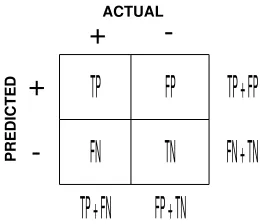
Figure 3.1: Confusion matrix for a 2-class problem
In supervised classification, Sensitivity, SN, and Sepecificity, SP, are defined using the confusion matrix in presented in figure (3.1) and are usually expressed as ([20]),
SN ≡The fraction of positive patterns predicted correctly by the model = T P
SP ≡The fraction of negative patterns predicted correctly by the model = T N
T N +F P.
However, in the context of gene finding, since the frequency of coding nucleotides in genomic DNA sequences is much less than the frequency of coding nucleotides (see [21]), the value of TN is generally much greater than the value of FP. As a result the calculated value of SP is noninformative. Therefore, instead, in bioinformatics litrature SP is computed as
SP ≡The fraction of predicted patterns that turns out to be positive = T P
T P +F P. (3.4)
Using this terminology, in classification problems where the input matrix is not sparse, and finding “positive” and “negative” patterns are equally important, the following two measures are also necessary.
nSN ≡The fraction of negative patterns predicted correctly by the model = T N
T N+F P. (3.5)
nSP ≡The fraction of predicted patterns that turns out to be negative = T N
T N+F N. (3.6)
3.3.1
Purity.
Let pij be the probability that an object in cluster i belongs to class j. Then purity
for the cluster i, pi, can be expressed as,
pi = max
j pij (3.7)
Note that the probability that an object in clusteri belongs to classj can be written as the number of objects of class j in cluster i, nij, divided by the total number of
objects in cluster i,ni, (i.e., pij=nij/ni.) Using this notation the overall validity of a
cluster i using the measure pi is the weighted sum of that measure over all clusters.
Hence,
purity = 1
N
k
X
i=1
nipi (3.8)
where,k is number of clusters and n is the total number of patterns. For our 2-class clustering problem equation (3.7) transforms to,
p1 =max(SP,1−SP) and p2 =max(nSP,1−nSP) (3.9) and after applying equations (3.4) and (3.3) to (3.8),
purity=max( T P +T N
T P +F P +T N +F N,1−
T P +T N
T P +F P +T N +F N). (3.10)
3.4
Unsupervised Cluster Validator
Unlike purity, unsupervised evaluation techniques like do not depend on external class information. These measures are often optimization functions in many cluster-ing algorithms. Sum-of-Squared-Error (SSE), measures the compactness of a scluster-ingle cluster and other measures evaluate the isolation of a cluster from other clusters. Un-fortunately, SSE is calculated in the input space which does not necessarilly reflect the goodness of the clustering in the feature space. In this section we develope an unsupervised cluster validator that works in feature space instead.
3.4.1
Kernel-Sum-of-Squared-Error (Kernel SSE)
Positive-definite kernels are related to another kind of kernels, callednegative-definite
kernels (see definition (7)) that are in turn related to Hilbert spaces through the
following theorem:
Theorem 12 A kernel, S, on set χ is nd iff ∃ a Hilbert Space, H, and a map
f :χ→H such that ∀x, y ∈χ,
S(x, y) =kf(x)−f(y)k2
Furthermore, if {S = 0} for all diagonal values, then √S is a metric on χ
The following lemma is the relationship between positive and negative-definite kernels.
Lemma 13 A kernel S is nd iff there exists a pd kernel, K, such that the following
relation holds:
S(x, y) = K(x, x) +K(y, y)−2K(x, y)
can rewrite S as following:
S(x, y) = kf(x)−f(y)k2
= hf(x), f(x)i+hf(y), f(y)i −2hf(x), f(y)i = K(x, x) +K(y, y)−2K(x, y)
This is a useful since geometrically S is a measure of distance between x and
y. Therefore, using lemma (13) for feature vectors x and x′ ∈ χ the inner cluster
sum-of-squared (see definition (10)), Ji,
Ji =
1
2nisi, (3.11)
where ni is the size of theith cluster and for any ndkernel S(x,x′),
si =
1
n2
i
X
x∈χi
X
x′∈χi
S(x,x′), (3.12) can be written as:
Ji =
X
x∈χi
K(x, x)− 1
ni
X
x∈χi
X
x′∈χi
K(x, x′). (3.13) Now, let, Km be a Gram matrix, where Km
ij = K(xi, xj) such that xi and xj are in
the mth cluster χm, then for any normalized pd kernel, K, (K(x, y) = 1 ⇔ x = y)
and a column vector of m ones, 1,
Ji =ni
1− 1
TKm1
n2
i
(3.14)
Similarly, for a non-normalizedpd kernel, K, ˜
Ji =trace(Km)−
1TKm1
ni
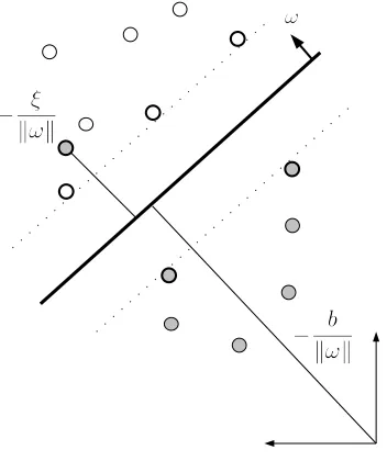
Figure 3.2: SVM on non-separable features
3.5
SVM-Relabeler Clustering Method
The SVM classification formulation is expanded to cluster a set of feature vectors with
noa priori knowledge of the features’ classification. Non-separable SVM guarantees
convergence at the cost of allowing misclassification. As depicted in the figure (3.2) the extent of slack is controlled through the regularization constant, C, to penalize the slack variable, ξ. If the random mapping
((x1, y1), ...,(xm, ym))∈χm×y
is not linearly separable when ran through a binary SVM, the misclassified features are more likely to belong to the other cluster. Moreover, by relabeling those heavily misclassified features and by repeating this process we arrive at a separation between the two clusters. As formulated in the core of SVM formulation this separation has the largest margin given the regularization constant,C. The basics of this procedure is presented in Algorithm (7), where ˆy is the new cluster assignment for x and θ is the resulting SVM model.
Algorithm 7 SVM-Relabeler
Require: Feature vectors: x
1: yˆ← Randomly chosen from{−1,+1}
2: repeat
3: θ ←doSV M(x,yˆ)
4: yˆ←doRelabel(x, θ)
5: untilyˆremains constant
of the geometry of the data2, in order to provide the doRelabel() procedure with the required model. After this procedure,doRelabel() reassignes some of the misclassified features to a the other cluster. If D(xi, θ) is the distance between xi feature and
the trained SVM hyperplane (see footnote explaining the projection), then heavily misclassified features, xj∈J, could be selected by comparing D(xj, θ) to D(xj′, θ) for
all j′ ∈ J. Algorithm (8) clarifies the basic implementation of this procedure by
introducing a confidence parameter, α, that is the bottom percentile of misclassified features beyond which is relabeled.
Algorithm 8 doRelabel1() Procedure
Require: Input vector: x
Cluster labeling: ˆy
SVM model: θ
Confidence Factor: α
1: Identify misclassified features:
ˆ
x+ ←k misclassified features with ˆy= +1 ˆ
x− ←l misclassified features with ˆy=−1
2: for all ith component of ˆx+ do
3: if D(ˆx+j, θ)> percentile(1−α) then
4: yˆ+i ← −1
5: end if
6: end for
7: for all ith component of ˆx−
do 8: if D(ˆx−j, θ)< percentile(α) then
9: yˆ−i ←+1
10: end if
11: end for
3.6
Refinement Methods Using Simulated
Anneal-ing
The SVM-Relabeler algorithm does not use an objective function and the hope is that by running the algorithm in its purest form the resulting clusters are reliable solutions. However, running this algorithm in this basic fashion does not consistently provide us with a satisfying clustering solution. In fact, the solution space can be divided into three sets: successful, local-optimum, and unsuccessful (see figure (4.3)).
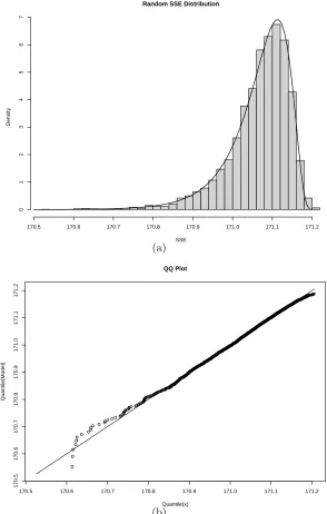
Trivially unsuccessful and the local optimum solutions are undesirable and should be ideally eliminated. Since, the solutions in the unsuccessful set are reasonably expected to be frequent in any experiment that calculates the the SSE of a randomly labeled data set, they can be simply eliminated by post-processing. For instance, in a similar experiment we have randomly labeled the dataset 5000 times and calculated the SSE distribution for the experiment. The resulting distribution has a good fit to Johnson’s SB distribution (see Appendix C) and is illustrated in the histogram of
figure (3.3). using a fitted distribution one can calculate the p-value of a given SSE. For example, SSE threshold of 170.5 (accidentally very unlikely) can be employed to eliminate the unsuccessful set.
To substantially reduce the local optimum solutions, however, thresholding does not scale well. One solution is a to use a simple hill climbing algorithm which is to run the algorithm for a sufficiently long number of iterations to find the solution with the lowest SSE value. To do this the algorithm (7) is ran repeatedly and randomly initialized every time. A solution is accepted as the best solution so far if it has a lower SSE than the previously recorded value.
It is observed that random perturbation by flipping each label at some proba-bility, ppert, is often sufficient to switch to another subspace where a better solution
could be found. (Note that ppert = 0.50 has the effect of random reinitialization and
pertpert = 1 flips the entire labels.) The hope is that perturbation with ppert 6= 0.50
Algorithm 9 SVM-Relabeler Using Simulated Annealing
Require: Input vector: x
SVM-Relabeler: doSV M() Initial system temperature: T
Annealing schedule: anneal() Perturbation schedule: pert() SSE function: SSE()
Random generator: rand()→(0,1)
1: initialize:
y←doSV M()
e←SSE(y)
t←T
2: repeat
3: perturb and evaluate:
ynext ←doSV M(pert(y))
enext ←SSE(ynext)
4: if (enext < e) W ((e < enext)V (rand()< exp(−enextt−e)))then 5: accept the new state:
y←ynext
e←enext
6: end if
7: anneal()
8: until threshold or maximum number of iteration reached
Random SSE Distribution
SSE
Density
170.5 170.6 170.7 170.8 170.9 171.0 171.1 171.2
0
1
2
3
4
5
6
7
(a)
170.5 170.6 170.7 170.8 170.9 171.0 171.1 171.2
170.5
170.6
170.7
170.8
170.9
171.0
171.1
171.2
QQ Plot
Quantile(x)
Quantile(Model)
(b)
Figure 3.3: (a) demonstrates the histogram and the fitted distribution by randomly labeling the 8GC/9GC data set using the Absdiff kernel (γ = 1.8) and computing SSE. The fitted Distribution is Johnson’s SB distribution (see Appendix) (γ = −5.5405,
SVM-Relabeler Results
SVM-Relabeler clustering algorithm is capable of clustering a wide range of data sets from simple 2-dimensional toy data (see Figure 4.1) sets to simple multi-dimensional data sets (e.g. Iris data set) to the complex Nanopore DNA hairpin data. The preliminary results were first published in [22] by this author and is now part of a more comprehensive presentation in this chapter.
4.1
Iris Data Set
−1.0 −0.5 0.0 0.5 1.0 −1.0 −0.5 0.0 0.5 1.0
Iteration: 1
−1.0 −0.5 0.0 0.5 1.0
−1.0
−0.5
0.0
0.5
1.0
Iteration: 2
−1.0 −0.5 0.0 0.5 1.0
−1.0
−0.5
0.0
0.5
1.0
Iteration: 3
Figure 4.1: SVM-Relabeler using a polynomial kernel
Sepal.Length
2.0 2.5 3.0 3.5 4.0 0.5 1.0 1.5 2.0 2.5
4.5 5.5 6.5 7.5 2.0 2.5 3.0 3.5 4.0 Sepal.Width Petal.Length 1 2 3 4 5 6 7
4.5 5.0 5.56.0 6.5 7.0 7.5 8.0
0.5
1.0
1.5
2.0
2.5
1 2 3 4 5 6 7
Petal.Width
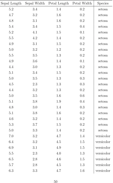
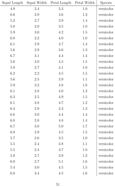
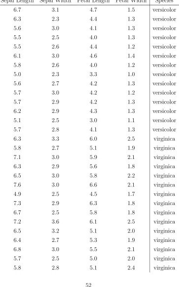
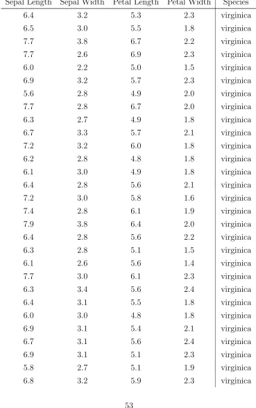
Table 4.1: Iris data set
Sepal Length Sepal Width Petal Length Petal Width Species
5.1 3.5 1.4 0.2 setosa
4.9 3.0 1.4 0.2 setosa
4.7 3.2 1.3 0.2 setosa
4.6 3.1 1.5 0.2 setosa
5.0 3.6 1.4 0.2 setosa
5.4 3.9 1.7 0.4 setosa
4.6 3.4 1.4 0.3 setosa
5.0 3.4 1.5 0.2 setosa
4.4 2.9 1.4 0.2 setosa
4.9 3.1 1.5 0.1 setosa
5.4 3.7 1.5 0.2 setosa
4.8 3.4 1.6 0.2 setosa
4.8 3.0 1.4 0.1 setosa
4.3 3.0 1.1 0.1 setosa
5.8 4.0 1.2 0.2 setosa
5.7 4.4 1.5 0.4 setosa
5.4 3.9 1.3 0.4 setosa
5.1 3.5 1.4 0.3 setosa
5.7 3.8 1.7 0.3 setosa
5.1 3.8 1.5 0.3 setosa
5.4 3.4 1.7 0.2 setosa
5.1 3.7 1.5 0.4 setosa
4.6 3.6 1.0 0.2 setosa
5.1 3.3 1.7 0.5 setosa
4.8 3.4 1.9 0.2 setosa
5.0 3.0 1.6 0.2 setosa
5.0 3.4 1.6 0.4 setosa