Automatic Change Detection Based on Edge Information Using Two Different Types of Ortho Image

(1)

1st_{ortho image (satellite)} ₂nd_{ortho image (aerial)}

1st_{edge image} ₂nd_{edge image}

Using Two Different Types of Ortho Image

Akira SASAGAWA

a *

, Shuto SUGAI

a,

, Mayumi NOGUCHI

a

a Geospatial Information Authority of Japan, [email protected] , [email protected], [email protected]

* Corresponding author

Abstract:

A new algorithm of automatic change detection for update of base map is presented. In conventional method, using two different types of ortho image, such as aerial photo and satellite image, makes detection quality worse due to the difference of each contrast, brightness, color balance and so on. To obtain robust result against such difference between two images, we introduce edge-vector technique. We applied this method using two ortho images derived from each aerial photo and satellite image. We have tested our method and confirmed a performance of the change detection by the interpretation test. In this paper, the detailed algorithm and the result of interpretation test are reported.

Keywords: Automatic Change Detection, Map Update, Ortho Image, Edge-vector

1. Introduction

1.1 Background

Geospatial Information Authority of Japan (GSI) is the national geospatial information authority. GSI prepared domestic base map, Fundamental Geospatial Data (FGD), in 2014. FGD covers all over Japan with 1:2500 scale level in city planning area and 1:25000 scale level in the other area. GSI is now updating FGD using various update sources. In updating stage, one of the important task for effective updating management is to find changed parts in all over Japan. However, GSI is now spending much time and effort on collecting a mass of material to find changed areas.

To find changed areas automatically, various methods for automatic change detection using two ortho images are proposed. While most of them are quite sensitive to difference of contrast, brightness, color balance and so on that these differences makes detection quality worse. To obtain robust results against the above differences, we developed the automatic change detection method based on edge-vector technique.

First we show the outline of our method. Next we describe edge-vector technique and details of each part. Then we show the result of interpretation test. We also give discussion on the features of our method.

1.2 Basic idea for detecting changes

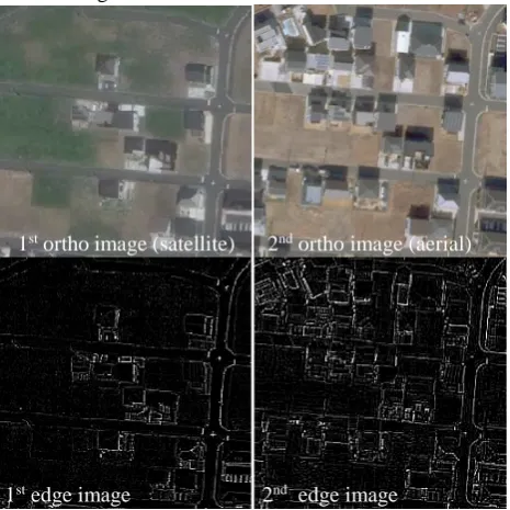
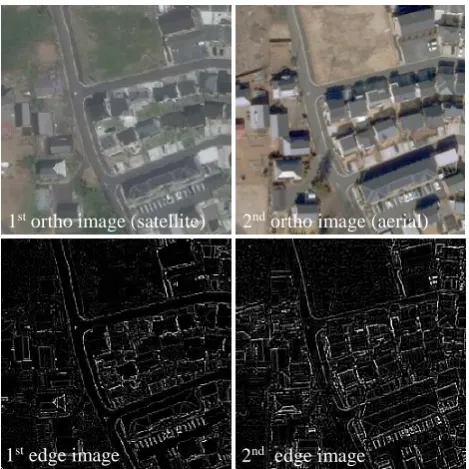
Figure 1 shows the case with changes, i.e. new houses are built in the second ortho image. In this case, much more edges exist in the second ortho image than in the first one. While Figure 2 shows the case without changes between two ortho images. In this case, it seems that there are also

no changes between two edge images. Note that the first ortho images are derived from satellite image and the second ortho images are derived from aerial photos. Due to this difference of image source, pixel values are completely different between two ortho images. On the other hand, an edge image is quite similar to the other edge image in non-changed area.

Thus, our proposed method focused on two edge images to detect changes.

(2)

1st_{ortho image} ₂nd_{ortho image}

a) Edge detection

1st_{edge vector} ₂nd_{edge vector}

c) Similarity calculation

Change detected image

a) Edge detection

1st_{edge image} ₂nd_{edge image}

b) Edge vectorization b) Edge vectorization 1st_{edge image} ₂nd_{edge image}

1st_{edge image (satellite)} ₂nd_{edge image (aerial)}

Histogram generation

Dimensional reduction

2nd_{edge image (aerial)} Figure 2. Example of ortho images and edge images

without changes

2. Method

2.1 Outline of proposed method

Figure 3 shows the outline of the proposed method. The proposed method requires two ortho images. First, it generates the both edge images. Then it generates both edge vectors in each small part of images. Next, Similarity between two edge vectors is calculated. Finally, change detected image is generated depending on the value of similarity. Each part is described in the following.

Figure 3. Flowchart of proposed method

2.2 Edge detection

As shown in a) of Figure 3, each edge image is generated from each ortho image. In this paper, the proposed method uses 3x3 Laplacian filter to generate edge image since it performed the best out of various edge detecting filter in preliminary experiment.

2.3 Edge vectorization

In order to calculate similarity between two edge images, we introduced edge-vector as a kind of feature value in b) of Figure 3.

Figure 4 shows the outline of edge-vector technique, how the proposed method generates an edge-vector from an edge image. First, each histogram, of which the range for domain is from 0 (black: non-edge) to 255 (white: obvious edge), is generated from each edge image. In other words, each histogram is equivalent to a 256-dimensional vector. Next, each 8 dimensional edge-vector is generated from each 256 dimensional histogram. In this paper, the proposed method applies linear dimensional reduction. This dimensional reduction can make similarity calculation robust. Since the small difference of shapes in each 256 dimensional histogram, caused by the difference of contrast, brightness, color balance and so on between two ortho images, can be reduced by reducing dimensions. Also this dimensional reduction has an effect for making similarity calculation faster.

Figure 4. Outline of edge-vector technique

2.4 Similarity calculation

As shown in c) of Figure 3, similarity is calculated using two edge vectors, 𝐸𝐸��⃗₁ and 𝐸𝐸��⃗₂. In this paper, the proposed method applies the cosine of the angle θ between 𝐸𝐸��⃗₁ and 𝐸𝐸2

(3)

Figure 6. Example of change detection; Left: 1st_{ortho image (satellite); Center: 2}nd_{ortho image (aerial photos); Right:} change detected image overlaid with 2nd_{ortho image}

Similarity =

𝐸𝐸

��⃗⋅𝐸𝐸

1

��⃗

2

�𝐸𝐸

��⃗��𝐸𝐸

₁

��⃗�

₂ = cosθ (1)

Note that there is a tendency to have much larger value in the first element of an edge vector than in the others. In this case, if there is obvious difference in several elements except the first element between two edge vectors, a change can’t be detected. To prevent from the above detection failure, cosine is calculated using second to eighth elements. Also Figure 5 shows the concept of the relation between a change and the angle between 𝐸𝐸��⃗₁ and 𝐸𝐸2

��⃗.

Finally, change detected image is generated based on each part of change index, which is classified into four stages depending on a value of each similarity. In this paper, we assigned the following values to each change index as shown in Table 1. Note that in this paper, single unit of change detected area is about 32 m2_{, equivalent to 64 pixel} square.

Figure 6 shows a practical example of a change detected image overlaid with 2nd ortho image. Residential development has not started yet in the 1st ortho image. While some roads, houses and commercial facilities are built in the second ortho image. As shown in the change detected image of Figure 6, the proposed method can roughly detect most of them in the change detected image.

Figure 5. Concept of relation between change and angle between two edge-vectors

Change index Similarity

High ~0.80

Medium 0.80~0.85

Low 0.85~0.90

None 0.90~1.00

Table 1. Correspondence between change index and similarity

3. Result

3.1 Test field and used image

The specification of the both ortho images applied to the proposed method is given in Table 2. We have tested our method using ortho images derived from a satellite image as the 1st_{ortho image and aerial photos as the 2}nd_ortho image. Both of the ortho images are observed over a test field in Tsukuba city, Ibaraki Pref., Japan where urban development is in progress. The interval of an image acquisition is about 21 months.

1st_{ortho image} ₂nd_{ortho image} Test field Tsukuba city, Ibaraki Pref., Japan Image

acquisition date

May, 2015 Feb, 2017 Image area 16km2_{(App. 2.5km*6.5km)} Ground

resolution

App. 50cm

Image Source Satellite image Aerial photo Table 2. Specification of used image

3.2 Change detected image

Appendix in the last two pages of this paper shows the result of the 1st_{ortho image, the 2}nd_{ortho image and the} change detected image overlaid with the 2nd_{ortho image,} including the whole area and specific parts of the image. Figure 7 in Appendix shows the whole area. In Figure 7, blue area (a) to (e) which are equivalent to Figure 8 to 12 show examples of detected some changes correctly. On the other hand, red area (f) in Figure 7 which is equivalent to Figure 13 shows detected errors caused by shadow.

3.3 Interpretation test

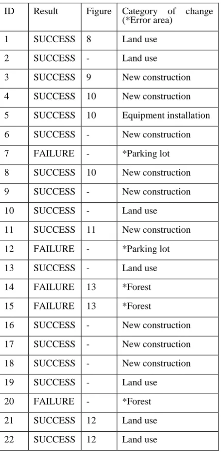
Interpretation test was carried out to measure the performance of the proposed method. In this paper, we checked change detected areas which has over 1000 m2 area whether a change exists or not by manual interpretation. Note that over 1000 m2 _{area is equivalent to} change detected areas which have at least 8 connected meshes in a change detected image.

(4)

ID Result Figure Category of change (*Error area)

1 SUCCESS 8 Land use

2 SUCCESS - Land use

3 SUCCESS 9 New construction 4 SUCCESS 10 New construction 5 SUCCESS 10 Equipment installation 6 SUCCESS - New construction 7 FAILURE - *Parking lot 8 SUCCESS 10 New construction 9 SUCCESS - New construction 10 SUCCESS - Land use

11 SUCCESS 11 New construction 12 FAILURE - *Parking lot 13 SUCCESS - Land use 14 FAILURE 13 *Forest 15 FAILURE 13 *Forest

16 SUCCESS - New construction 17 SUCCESS - New construction 18 SUCCESS - New construction 19 SUCCESS - Land use

20 FAILURE - *Forest

21 SUCCESS 12 Land use 22 SUCCESS 12 Land use Table 3. Result of interpretation test

Table 3 shows the result of the interpretation test. Some of them are shown as a result of change detection in figures of Appendix.

After all, 17 of 22 are correctly detected. On the other hand, 5 of 22 are incorrect, actually no changes by manual interpretation test while the proposed method detected as a change.

In these 5 incorrect cases, 3 of 5 are in a forest area so that edge change is incorrectly detected caused by complex shape of shadow by trees. Also 2 of 5 are in a parking lot so that difference in layout of cars is detected as a change. From this result of the interpretation test, it became clear that many changes of newly built construction and land use could be detected by the proposed method in spite of the difference of contrast, brightness, color balance and so on between two ortho images. While complex shape of shadow and different layout of cars caused detected errors.

4. Conclusion and future work

In this paper, we proposed new automatic change detection method based on edge information. We introduced “edge-vector technique” to detect changes between two ortho images and confirmed robustness against difference of contrast, brightness, color balance and so on of two images. From the interpretation test, the proposed method detected 17 of 22 changes correctly. Also it became clear that complex shape of shadow and different layout of cars caused detected errors.

To reduce detected errors, we will research more to make the proposed method better. Also more detailed performance assessment is required since we have evaluated a number of detected errors in this paper but not a number of miss detection.

5. Acknowledgement

The authors thank all colleagues in Geospatial Information Authority of Japan for their valuable comments.

6. References

A. Gruen, S.Kocaman, K.Wolff, 2007. "CALIBRATION AND VALIDATION OF EARLY ALOS/PRISM IMAGES" Journal of the Japan Society of Photogrammetry and Remote Sensing, Vol.46, No.1, pp.24-38 (accepted)

A. Sasagawa, 2007. "Automatic Change Detection Using Pair of PRISM Triplet Images" Proc. The First Joint PI symposium of ALOS Data Nodes for ALOS Science Program in Kyoto, pp.24-38

A. Sasagawa, K. Watanabe, S. Nakajima, K.Koido, H.Ohno, H. Fujimura, 2008. “Automatic Change Detection Based on Pixel-change and DSM-change” The International Archives of the Photogrammetry, Remote Sensing and Spatial Information Sciences, Beijing, China, Vol. XXXVII, Part B7, pp. 1645-1650. (accepted) A. Sasagawa, E. Baltsavias, Sultan Kocaman Aksakal, Jan

(5)

Figure 7. Whole result of change detection; Left: 1st_{ortho image (satellite); Center: 2}nd_{ortho image (aerial photos);} Right: change detected image overlaid with 2nd_{ortho image}

(a) (a) (a)

Figure 8. Result of change detection at (a) in Figure 7; Left: 1st_{ortho image (satellite); Center: 2}nd_{ortho image (aerial} photos); Right: change detected image overlaid with 2nd_{ortho image}

(b) (b)

(b)

Figure 9. Result of change detection at (b) in Figure 7; Left: 1st_{ortho image (satellite); Center: 2}nd_{ortho image (aerial} photos); Right: change detected image overlaid with 2nd_{ortho image}

1st_{ortho image (satellite)}

2nd_{ortho image (aerial)}

(c) (c) (c)

(f)

(d) (d)

(d)

(e) (e)

(e)

(f) (f)

(6)

Figure 10. Result of change detection at (c) in Figure 7; Left: 1st_{ortho image (satellite); Center: 2}nd_{ortho image (aerial} photos); Right: change detected image overlaid with 2nd_{ortho image}

Figure 11. Result of change detection at (d) in Figure 7; Left: 1st_{ortho image (satellite); Center: 2}nd_{ortho image (aerial} photos); Right: change detected image overlaid with 2nd_{ortho image}

Figure 12. Result of change detection at (e) in Figure 7; Left: 1st_{ortho image (satellite); Center: 2}nd_{ortho image (aerial} photos); Right: change detected image overlaid with 2nd_{ortho image}

Figure 13. Result of change detection at (f) in Figure 7, example of extraction error caused by shadow; Left: 1st_ortho image (satellite); Center: 2nd_{ortho image (aerial photos); Right: change detected image overlaid with 2}nd_{ortho image} 1st_{ortho image (satellite)}

1st_{ortho image (satellite)}

2nd_{ortho image (aerial)}