The Prevalence and Course of Idiopathic Toe-Walking in 5-Year-Old Children

(1)

RESEARCH SECTION

Mike G. Dosskey is a research ecologist and Todd Kellerman is a GIS specialist with the US Forest Service, USDA National Agroforestry Cen-ter in Lincoln, Nebraska. Surendran Neelakan-tan is a graduate student in the Department of Computer Science, University of Kentucky in Lexington. Tom G. Mueller is an agronomic data researcher with Deere & Company in Urbandale, Iowa. Matt J. Helmers is a professor in the De-partment of Agricultural and Biosystems Engi-neering at Iowa State University in Ames, Iowa. Eduardo Rienzi is a postdoctoral scholar in the Department of Plant and Soil Sciences, Universi-ty of Kentucky in Lexington.

AgBufferBuilder: A geographic information

system (GIS) tool for precision design and

performance assessment of filter strips

M.G. Dosskey, S. Neelakantan, T.G. Mueller, T. Kellerman, M.J. Helmers, and E. Rienzi

Abstract: Spatially nonuniform runoff reduces the water quality performance of con-stant-width filter strips. A geographic information system (GIS)-based tool was developed and tested that employs terrain analysis to account for spatially nonuniform runoff and pro-duce more effective filter strip designs. The computer program, AgBufferBuilder, runs with ArcGIS versions 10.0 and 10.1 (Esri, Redlands, California) and uses digital elevation models to identify detailed spatial patterns of overland runoff to field margins. The tool then sizes fil-ter dimensions according to those patfil-terns using buffer area ratio relationships. The resulting design is larger along segments where more runoff flows and smaller along segments where runoff is less and delivers a constant level of trapping efficiency around the field margin for sediment and sediment-bound pollutants. The tool also can estimate trapping efficiency of existing filter strips or hypothetical configurations. In a validation test, estimates of sediment trapping efficiency using the tool’s assessment function compared closely to measurements taken on large field plots in central Iowa. Using AgBufferBuilder, designs developed for a sample of fields in the midwestern United States were estimated to trap nearly double the sediment, on average, during a design storm than constant-width configurations having equiv-alent total filter area. AgBufferBuilder can be used to bolster environmental performance of filter strips where runoff is spatially nonuniform. The AgBufferBuilder tool is publicly avail-able on the websites http://www2.ca.uky.edu/BufferBuilder and http://nac.unl.edu/tools/ AgBufferBuilder.

Key words: digital elevation model—nonpoint pollution—precision conservation—terrain analysis—vegetative buffer—water quality

Vegetative filter strips are installed along margins of crop fields to protect and improve water quality in agricultural watersheds. Filter strips reduce the load of sediment, nutrients, and other pollutants that reach waterways by slowing overland run-off flow from fields and promoting sediment deposition. Typically, they are designed to have a constant width (in the direction of water flow) along a field margin and for field runoff to be uniformly dispersed into and across the entire filter strip (NRCS 2013). Several methods have been devel-oped for determining appropriate widths for filter strips treating spatially uniform runoff (Wong and McCuen 1982; Flanagan et al. 1989; Nieswand et al. 1990; Dillaha and Hayes 1991; Suwandono et al. 1999; NRCS 2007; Dosskey et al. 2008).

In many situations, however, overland run-off is not uniformly distributed and instead moves as concentrated flow to and across only portions of a field margin (Dillaha et al. 1986, 1989; Fabis et al. 1993; Dosskey et al. 2002; Pankau et al. 2012). A constant-width filter strip is less effective under these con-ditions than if the flow is uniform (Dickey and Vanderholm 1981; Dillaha et al. 1988, 1989; Daniels and Gilliam 1996; Dosskey et al. 2002). For example, a study of farms in eastern Nebraska estimated sediment trap-ping efficiency of existing vegetative filters under observed nonuniform runoff flow to be less than half of what would be expected if runoff flow was uniform (Dosskey et al. 2002). In this study, trapping efficiency was reduced along segments of the filters receiv-ing concentrated flows, while other segments

received little or no runoff and contributed little to reducing sediment export from these farms. Current filter strip standards require runoff to be uniform and for concentrated flow to be dispersed before it enters the fil-ter strip (NRCS 2013). Methods for doing so include grading the field or constructing spreaders, but these activities can add substan-tial cost. A more cost-effective design would simply vary the dimensions of filter strip according to the amount of runoff received— larger where runoff is greater and smaller where runoff is less (Dosskey et al. 2005).

A design method has been proposed for sizing filter strips that can account for spa-tially nonuniform overland runoff (Dosskey et al. 2011). This method sizes different seg-ments of a filter strip along a field margin in relation to the size of field area that drains to each segment (i.e., buffer area ratio). This approach can account for contributing areas having varying dimensions and irregu-lar shapes. Additional information on slope, soil texture, and soil cover condition help to define the ratio, which provides a specific user-selected level of pollutant trapping effi-ciency. Using this method, the size of each segment of a filter strip is determined inde-pendently. This method is quantitative and applicable to both uniform and nonuniform runoff conditions, but is particularly advan-tageous where runoff is nonuniform.

Manual application of this method, how-ever, can be slow and laborious if the field margin is divided into many segments. Contributing area and filter size must be determined separately for each one of the segments. This task could be made much quicker and easier by automating it with computer-aided terrain analysis. Segments, contributing areas, and slopes could be determined by analysis of a digital elevation doi:10.2489/jswc.70.4.209

www.swcs.org

70(4):209-217

(2)

system (GIS). This procedure could quickly calculate filter sizes and map them for many segments along a field margin. Technology enhancement would facilitate perfor-mance-based design and implementation of more effective filter strips in landscapes where runoff is nonuniform.

The automated method could be further enhanced by adding functionality for assess-ing the performance level of existassess-ing filter strips and hypothetical ones. Such an assess-ment would involve simply using terrain analysis to determine the buffer area ratio provided by the existing or hypothetical fil-ter in each segment, and then calculating the associated trapping efficiency of each one. Then, trapping efficiency of the whole filter strip could be calculated as the contributing area-weighted average trapping efficiency (CAWATE) of all segments. This procedure would use the same input data as the design methodology, with the addition of a digital map indicating the location of the existing or hypothetical filter strip, and utilize the same quantitative relationships between buffer area ratio and trapping efficiency as used for design. The results could be used to estimate the trapping efficiency of past installations and to evaluate comparative performance of alternative future designs.

The objectives of this study were to (1) develop a GIS-based procedure for design-ing and assessdesign-ing performance of filter strips based on the methodology of Dosskey et al. (2011), (2) validate results produced by the GIS procedure by comparing them to field measurements, and (3) demonstrate the utility of the GIS procedures by comparing performance of spatially variable designs to that of constant-width configurations of the same overall size.

Materials and Methods

The Design Model. The design model (Dosskey et al. 2011) guides the user to select a buffer area ratio that will achieve a desired level of trapping efficiency under the following given set of field conditions: slope, soil texture, tillage and residue cover, and the type of pollutant to be controlled. Briefly, the model is a simplification of the process-based Vegetative Filter Strip Model (VFSMOD version 1.04; Muñoz-Carpena and Parsons 2000, 2005; Muñoz-Carpena et al. 2007). To develop it, repeated simula-tions were run to quantify the relasimula-tionships

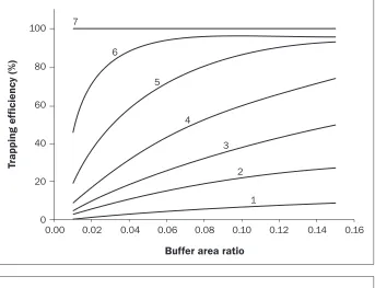
ratio for a grass filter strip receiving overland runoff from a crop field during a large rainfall event (61 mm [2.4 in] in one hour). The simulations included different combinations of soil texture class, slope, and soil cover condition (Universal Soil Loss Equation [USLE] cover and management factor [C factor]), factors that are well known to sig-nificantly affect runoff and sediment loads from fields and trapping capabilities of fil-ter strips (Wischmeier and Smith 1978; Dosskey 2001; Helmers et al. 2002). The results for each scenario were fit to an equa-tion by nonlinear regression. Seven of those regression lines were selected that illustrate the range of possible relationships between trapping efficiency and buffer area ratio (figure 1). Then, rules were developed to estimate which of those seven relationships would be most appropriate for any given site based on its slope, soil texture, soil cover condition, and pollutant type (sediment or sediment-bound).

In a manual application of the design model, the field margin is divided into sev-eral segments, and the contributing area to each one is determined visually in the field with or without the aid of a topographic map. Then, a filter strip is sized for each seg-ment. There are two steps for determining which line in figure 1 to use for a given seg-ment of field margin. First, choose an initial reference line. Second, adjust to a different line depending on how much the actual site conditions and pollutant type differ from those represented by the initial reference line (table 1) according to rules in table 2. Use this final selected line in the graph to deter-mine the buffer area ratio that corresponds to the desired level of trapping efficiency (i.e., percentage of runoff load retained within the filter area). Multiply that ratio by the size of the contributing area to determine the appropriate size for the filter area along that segment of field margin. This process is repeated for each segment of field margin.

Coupling the Design Model to Terrain Analysis in a Geographic Information System. The design process was automated by employing terrain analysis in a GIS. Use of computers can speed the design process where there are many segments and provide an objective framework for applying the design model.

A computer program based on the design model, called AgBufferBuilder version 1.0,

ware (versions 10.0 and 10.1 with SP5; Esri, Redlands, California). It was programmed in Python coding language to enable efficient integration into the ArcGIS analytical archi-tecture, although some algorithms remain in ArcGIS Model Builder format, which is eas-ier for adding functionality. In the GIS, the user draws the field margin on a digital aerial photo of the field. The program uses the grid structure of a DEM to divide the field mar-gin into segments. One segment equals one grid cell. The Flow Accumulation and Slope functions of ArcGIS are used to determine the size and average slope of contributing area to each segment. Surface soil texture class and soil cover condition (USLE C fac-tor) are considered constant for the entire field. There are three categories of soil tex-ture (fine, medium, and coarse, as defined in the caption of table 2). There are two levels of soil cover condition, USLE C factor 0.50 and 0.15, values which are representative of fresh contour plow tillage and conservation tillage, respectively, with moderate crop residue (Wischmeier and Smith 1978). The computer program automates the rules for selecting the appropriate design line (table 2) and employs its equation (table 3) to calcu-late the filter area required in each segment’s contributing area to deliver the user-se-lected level of trapping efficiency. Filter area is converted to numbers of grid cells and placed in contributing area cells closest to the field margin. This process is repeated for all field margin segments. The result is a design for a filter strip that will provide an approximately constant level of trapping efficiency along an entire field margin. The level of trapping efficiency is then recalcu-lated because rounding algorithms (e.g., to the nearest whole cell) results in a somewhat different value than the user-selected input value. It is calculated as the CAWATE of the filter-filled grid cells. The program then creates a GIS map showing the locations of filter-filled grid cells that, when overlaid on an aerial photo, can be used to lay out the location of filter strips on the ground around the entire field. A table of statistics is pro-duced that includes the total field area, total filter area, and the CAWATE of the entire filter strip.

Adding Functionality for Assessing Performance of User-Defined Filter Strips. Functionality was added to AgBufferBuilder that enables predicting trapping efficiency

www.swcs.org

70(4):209-217

(3)

Figure 1

Relationships between pollutant trapping efficiency and buffer area ratio for seven different conditions during a rainfall event of 61 mm in one hour. The conditions represented by each line are listed in table 1. The equations for each line are listed in table 3.

Trapping

ef

ficiency

(%)

100

80

60

40

20

0

0.00 0.02 0.04 0.06 0.08 0.10 0.12 0.14 0.16 Buffer area ratio

7

6

5

4

3

2

1

Table 1

Simulation conditions corresponding to each line in figure 1. The Universal Soil Loss Equation (USLE) C factor is the cover and management factor of the USLE (Wischmeier and Smith 1978).

Line number Material Slope (%) Soil texture class USLE C factor

7 Sediment 2 Fine sandy loam 0.50

6 Sediment 2 Silty clay loam 0.15

4 Water 2 Fine sandy loam 0.50

3 Water 10 Fine sandy loam 0.50

1 Water 10 Silty clay loam 0.50

Table 2

Rules for adjusting from a reference line number in figure 1 to a line number representing the actual field site based on how much the actual field site conditions differ from those for the reference line. Soil texture classes are divided into three broad categories: (1) coarse (sandy loam, sandy clay loam, and fine sandy loam), (2) medium (very fine sandy loam, loam, and silt loam), and (3) fine (clay loam, silty clay loam, and silt). The Universal Soil Loss Equation (USLE) C factor is the cover and management factor of the USLE (Wischmeier and Smith 1978).

Variable Adjustment rule

Slope 1 Line higher (+1) for each 2.5% lesser slope 1 Line lower (–1) for each 2.5% greater slope Soil texture category 1 Line higher (+1) for each category coarser

1 Line lower (–1) for each category finer

USLE C factor 1 Line higher (+1) for each 0.35 lower C factor 1 Line lower (–1) for each 0.35 higher C factor Pollutant type 1 Line lower (–1) from sediment to sediment-bound

of existing or hypothetical filter strips. In this procedure, the user draws the field margin where it would be if there was no filter strip, then draws the filter area poly-gons, either existing or hypothetical. The filter area polygons are converted to rasters by AgBufferBuilder in the DEM grid. Then, using the same algorithms as in the design procedure, the program determines contrib-uting area and buffer area ratio that exists for each segment along the field margin, and the appropriate equation (table 3) to assess each one based on slope, soil texture class, soil cover condition, and pollutant type. The trapping efficiency is calculated for each seg-ment, and then CAWATE is calculated for the field as a whole.

The AgBufferBuilder tool, which includes both the design and the performance assess-ment functions, is publicly available on the websites http://www2.ca.uky.edu/ BufferBuilder and http://nac.unl.edu/tools/ AgBufferBuilder.

Validating AgBufferBuilder. The accuracy of AgBufferBuilder was investigated by com-paring sediment trapping efficiency of filter strips measured in the field with that esti-mated using AgBufferBuilder. The field site is located in Jasper County in south central Iowa, a region of loess topsoils and rolling topography. The field measurements were made as part of the plot study described in Zhou et al. (2010), Helmers et al. (2011), and Zhou et al. (2014). This present inves-tigation focused on seven of their plots. The plots are 0.5 to 2.9 ha (1.2 to 7.1 ac) in size and each one encompasses a natural topo-graphic catchment within a large crop field. Each plot is roughly teardrop shaped and overland runoff converges to a narrow point where it leaves the field. Average slope of the plots ranges from 6.6% to 10.5%, the surface soil texture is borderline silt loam to silty clay loam, and the surface soil has a bulk density of approximately 1.41 g cm–3_{(0.81 oz in}–3_). All plots were converted out of bromegrass

(Bromus) by mulch-tilling and into no-till

corn (Zea mays L.)–soybean (Glycine max) rotation four growing seasons prior to the measured storm event. Each growing season, crops were planted on the contour, and crop residues were left in the field. Three of the plots contained no filter strip (control plots) and four plots contained filter strips covering 10% of the plot area, either all at the footslope or divided equally between the footslope and a contour strip at midslope. Helmers et al.

www.swcs.org

70(4):209-217

(4)

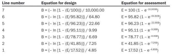
Equations corresponding to each line in figure 1. In the equations, E is the trapping efficiency

percentage and B is the buffer area ratio, or ratio of buffer area to contributing area. Line number Equation for design Equation for assessment

7 B = {– ln [1 – (E/100)]} / 10,000.00 E = 100 (1 – e–10,000B₎

6 B = {– ln [1 – (E/95.82)]} / 64.80 E = 95.82 (1 – e–64.80B₎

5 B = {– ln [1 – (E/96.23)]} / 22.66 E = 96.23 (1 – e–22.66B₎

4 B = {– ln [1 – (E/95.11)]} / 9.99 E = 95.11 (1 – e–9.99B₎

3 B = {– ln [1 – (E/78.77)]} / 6.69 E = 78.77 (1 – e–6.69B₎

2 B = {– ln [1 – (E/41.85)]} / 7.25 E = 41.85 (1 – e–7.25B₎

1 B = {– ln [1 – (E/17.52)]} / 4.85 E = 17.52 (1 – e–4.85B₎

(2011) detected no significant performance difference between these two placement configurations. Two other plots had 10% fil-ter area, but had missing data for the storm event evaluated in this present study.

Sediment trapping was evaluated for one rainfall event. The event occurred on August 8, 2010, and produced 40.4 mm (1.6 in) in one hour onto soil that was wet from 75 mm (2.9 in) of rainfall in the previous five days. This was the only rainfall event in growing seasons 2007 to 2012 that matched all six of the model criteria: a single, large, one hour-long event, on previously wet soil, that was sampled entirely within one mid-night-to-midnight measurement period, and for which data was successfully collected on all three control plots and at least three of the possible six filter plots. During the rain-fall event, runoff from each plot was guided through an H-flume and Isco 6712 auto-mated water sampler. Flow measurements were made every five minutes and water samples were collected for sediment con-centration for every 1.024 mm (0.040 in) of runoff. From data on total flow and flow-weighted mean concentration, the sediment load leaving each plot was calculated for the entire rainfall event.

Sediment trapping efficiency of each fil-ter plot was calculated by the difference in sediment loss between the filter plot and the mean sediment loss from the control plots (no filter) expressed as a percentage of mean sediment loss from the control plots. At the time of the measured storm event, the crop portions of plots contained a fully grown stand of corn and the filter strip portions contained a well-developed, diverse mixture of native prairie grasses and forbs.

For comparison to the field measured val-ues, AgBufferBuilder version 1.0 for ArcGIS 10.1 was used to estimate sediment trapping efficiency of the filter strips on each of the four filter plots. Three GIS layers were created

for each plot: a DEM, a plot border vector, and a filter strip polygon. First, a DEM having a 3 m (9.8 ft) raster grid was obtained from the US Geological Survey (USGS) National Elevation Dataset (http://ned.usgs.gov). The DEM was derived from LiDAR data col-lected from 2007 to 2008. Second, the 3 m grid map was subsequently resampled to a 1 m (3.3 ft) grid using bilinear interpolation and overlain on a plot border map created from a real-time kinematic (RTK) survey of each plot. The ArcGIS Flow Accumulation function was run to identify the border grid cell to which most of plot drains (i.e., pour point). Some grid cells within the RTK survey boundary did not flow to the pour point according to the DEM, so the ArcGIS Watershed Function was run on the pour point to create a single contributing area based on the DEM. Then, the watershed ras-ter was converted into a border vector for input to AgBufferBuilder. Third, a filter strip polygon was drawn at the footslope of the contributing area polygon equivalent in size to a buffer area ratio of 0.10, or 10% of the contributing area. Since all areal determi-nations are made on the DEM raster to the nearest whole grid cell, resampling the DEM to a smaller grid size enabled greater preci-sion in delineating boundaries and matching plot sizes and buffer area ratios on the DEM to those existing in the field. The 1 m grid size is similar to the width of H-flumes (1.16 and 1.45 m [3.8 and 4.7 ft]) that formed the outflow points of the field plots. Resampling does not technically increase the precision of the elevation data, but it creates useful inter-polations that can enhance identification of overland flow pathways (Pike et al. 2012).

The remaining input parameters were a USLE C factor for a “no-till” field and a soil texture class of “coarse.” While the selection of “coarse” for soil texture does not accu-rately describe the borderline silty clay loam (“fine”) or silt loam (“medium”) soils at the

site, it was selected as an adjustment for the smaller rainfall event (40.4 mm [1.6 in] in one hour) than the model reference (61 mm [2.4 in] in one hour) according to the guideline in Dosskey et al. (2011). The AgBufferBuilder version 1.0 program does not have a separate input variable for size of rainfall event, but this adjustment to the soil texture parameter will have the identical effect on results from the model. The accuracy of AgBufferBuilder was evaluated by comparing its estimates of sediment trapping efficiency to the measured value for each filter plot.

Finally, total error in estimates using AgBufferBuilder was partitioned into the following two main sources: error in the core model (Dosskey et al. 2011) and error in the algorithms used in converting the model to a GIS platform. Error in the algo-rithms was evaluated by comparing estimates of trapping efficiency using AgBufferBuilder with estimates determined manually using the core model. The remaining error would be attributable to the core model.

Case Studies of Designs and Assessments. The AgBufferBuilder design and assessment procedures were applied to six crop fields in the midwestern United States. In this region, overland runoff from cultivated fields is a major source of sediments and associated pollutants to waterways. The study fields were selected ad hoc to demonstrate the use of AgBufferBuilder and provide an exam-ple of its utility. Digital aerial orthophotos of the fields were obtained from the USDA Natural Resources Conservation Service (NRCS) Geospatial Data Gateway website (http://datagateway.nrcs.usda.gov). Digital elevation models having approximately 10 m (32.8 ft) grid spacing were obtained from the USGS National Elevation Dataset web-site (http://ned.usgs.gov) and resampled to a 5 m (16.4 ft) grid size.

For each field, an AgBufferBuilder design was produced. Then, a hypothetical filter strip polygon of constant width was drawn along the downhill margins of the field so that the total filter area was equal to that produced by the design program. The CAWATE value of the constant-width con-figuration was assessed and then compared to that of the AgBufferBuilder-designed configuration. The difference provides an indication of the importance of accounting for spatial patterns of runoff in the perfor-mance of filter strips.

www.swcs.org

70(4):209-217

(5)

Results and Discussion

The design model of Dosskey et al. (2011) was successfully programmed into computer code to enable users to more quickly and easily design a filter strip that will provide a constant, user-defined level of trapping efficiency around a crop field. The proce-dure employs a DEM grid to divide the field margin into short segments and enables the program to design filter strips for each segment based on the size and slope of its contributing area, its soil texture, its USLE C factor, the pollutant type (sediment or sediment-bound), and the level of trapping efficiency that is desired. An analogous pro-cedure was also successfully developed that enables the user to estimate the whole-field trapping efficiency of an existing or other user-defined filter strip configuration. The resultant program, called AgBufferBuilder version 1.0, was tested successfully for use with ArcGIS version 10.1 and ArcGIS version 10.0 with SP5. The design and assessment procedures of AgBufferBuilder were demonstrated on several crop fields in Kentucky, Illinois, Iowa, and Missouri.

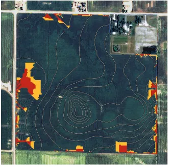
Example of the Design Procedure. An example of an AgBufferBuilder-designed filter strip is shown in figure 2 for a field in Madison County, Illinois. The aerial photo-graph shows the 59.5 ha (147 ac) crop field and 1 m (3.3 ft) elevation contours. The sin-uous contours suggest that runoff does not distribute uniformly to the margin around this field and, consequently, the designed filter strip has a highly variable configura-tion—larger where there is more runoff and smaller where there is less. The designed filter strip is expected to provide a constant trapping efficiency along the entire field margin. Sediment trapping efficiency would be 47% (in red), which increases to 72% by adding the area in yellow, under the design rainfall event (61 mm [2.4 in] in one hour) onto fine-textured soil soon after the field is tilled. The design image can be used in the field to lay out the filter area, and the statis-tics can be used to calculate installation costs and incentive payments.

The value for CAWATE, in theory, should be equal to the trapping efficiency value specified in the input because that value was used to determine filter area require-ment for every contributing area. However, it may be somewhat lower than the input value for two reasons. First, the calculated filter area requirement is rounded to the

Figure 2

A digital aerial orthophoto of a 59.5 ha field in Madison County, Illinois, showing 1 m contours and AgBufferBuilder-designed filter locations in a 5 m grid for achieving a constant 47% sedi

-ment trapping efficiency (in red) around the field margin, which increases to 72% by adding the

area in yellow. This field was assumed to be plow tilled and have a fine soil texture.

nearest whole cell. Rounding is expected to balance out approximately among many contributing areas between rounding up from 0.5 cell and rounding down from 1.5 cell. However, rounding produces bias for field margin cells having a calculated filter area requirement that is between 0 and 0.5 cell. On balance, these cells would have an average of 0.25 cell of filter area, but end up containing none in the design output. As a consequence, the designed filter area (cells filled with filter) will have less than the total calculated filter area requirement and, thus, will have a lower CAWATE value than the design input value. Second, contributing areas of some border cells may have severe slope and soil texture conditions that would render a filter strip practically incapable of achieving a high specified level of trap-ping efficiency (lines 1 to 3 in figure 1). In these cases, the program will fill the entire contributing area with filter, and assign the

maximum value (asymptote of the equa-tion) for that line. These contributing areas will, then, have a trapping efficiency value less than the specified input value and pull down the CAWATE value. For example, the larger design scenario in figure 2 (in yellow) had an input trapping efficiency of 75%, but the output CAWATE value was 72%. Use of a finer grid size will reduce the cell-rounding effect and bring the output CAWATE value of a design closer to the specified input value.

Locations along field margins where rel-atively more or less filter area is located do not change materially with a change in soil texture, tillage system, or by specifying a different input level of pollutant trapping efficiency. In general, only the total amount of filter area changes. For conditions that increase the runoff load (i.e., steeper slopes, finer-textured soils, and higher C factor) or a higher input trapping efficiency is selected,

www.swcs.org

70(4):209-217

(6)

the designed filter strip simply expands far-ther uphill. However, a few more grid cells may also appear elsewhere at the field mar-gin as the threshold for filling cells with filter area, 0.5 cell, is met. These features are exemplified in figure 2 where the input trapping efficiency was increased from 50% to 75% (i.e., CAWATE of the design output was 47% and 72%, respectively).

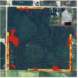
Example of the Assessment Procedure. An example of the AgBufferBuilder assess-ment procedure is depicted in figure 3. In this example, a 20 to 25 m (65.6 to 82 ft) wide filter strip was hand-drawn along the margin of the same field shown in figure 2. Filter strip polygons were placed where the design procedure indicated that most run-off would leave the field, and it was drawn to have the same total area (4 ha [10 ac]) as the AgBufferBuilder-designed filter that provides 72% sediment trapping efficiency. Running the assessment function on this constant-width filter strip returned a sed-iment CAWATE value of 35%, or about 35% of the sediment delivered to the field margin from this field would be trapped by this filter strip. In this way, the user can esti-mate the whole-field trapping efficiency of various alternative sizes and configurations of filter area, including that of existing filter strips. When applied after running the design procedure, the user can develop and assess alternative designs with knowledge of where the most effective locations would be and what level of performance could be attained for a given amount of filter area.

Irregular and fragmented design configura-tions produced by AgBufferBuilder will not be easily laid out in the field, nor be compatible with traditional farming equipment. However, complex field layouts are now becoming more feasible with precision agricultural technolo-gies such as GPS, guidance systems, and row or section control technologies on planters and applicators (Dosskey et al. 2005; Delgado et al. 2011). The assessment procedure in AgBufferBuilder enables a planner to evaluate alternative designs that can provide a better fit to the landowner’s circumstances.

Some planning needs may require know-ing the total mass of sediment, rather than percentage of it, that would be trapped by the filter during a design storm. It could be estimated for a whole field by using a model such as the Revised Universal Soil Loss Equation (RUSLE; Renard et al. 1997) to estimate the total mass of sediment in runoff

A digital aerial orthophoto of a 59.5 ha field in Madison County, Illinois, showing 1 m contours and a hypothetical constant-width filter strip (in yellow) in a 5 m grid having the same total area as the AgBufferBuilder design (in red) for plow tillage and fine soil texture. The sediment trapping efficiency of the constant-width filter strip is estimated to be 35%, while the AgBuffer

-Builder design is estimated to be 72%.

to the field margin, and then multiplying by the CAWATE value from AgBufferBuilder for any given design. This approach could be useful for scaling adoption incentives or credits to level of performance.

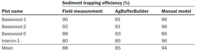
Validation Results. For the test rainfall event, measured sediment trapping efficiency of the filter strip plots averaged 88% and ranged from 80% to 92% among the four plots (table 4). By comparison, AgBufferBuilder estimated trapping efficiencies to average 85% and range from 81% to 91% (table 5). AgBufferBuilder overestimated correspond-ing field-measured values for two plots by 1% (Basswood-1) and 5% (Interim-1) and underestimated values on the other two plots by 11% (Basswood-2) and 5% (Basswood-5). While AgBufferBuilder estimates were off by as much as 11% for individual contribut-ing areas, the collective error was only 3%. Since a filter strip normally would have many

contributing areas averaged together, this average error may represent a better gauge of AgBufferBuilder accuracy for an entire fil-ter strip. Based on these results, the accuracy of AgBufferBuilder is reasonably good with only a minor bias toward underestimation of sediment trapping efficiency.

Manual application of the core model on the filter plots estimated sediment trapping efficiency to average 94% and range from 86% to 96% (table 5). AgBufferBuilder pro-duced lower values than the manual model did on all four plots by 5%, 15%, 3%, and 11%. These results indicate that the algorithms used to convert the core model into the GIS platform lead to underestimation of trapping efficiency values that would be produced by its core model alone. In this study, however, the net result was to bring AgBufferBuilder estimates closer in line to the field measured values than the core model estimates were.

www.swcs.org

70(4):209-217

(7)

Table 4

Field-measured sediment trapping efficiencies of large filter strip plots. Trapping efficiencies were determined for one large rainfall event (40.4 mm in one hour on August 8, 2010) on field plots covered by contour planted no-till corn either entirely (No Filter) or with 10% of their area covered with grass filter strip (10% Filter). The field plot descriptions and sediment loss data were collected as part of the study reported in Helmers et al. (2011).

Plot description Field measurement Size Slope Max. slope Sediment Trapping Plot name (ha) (%) length (m) loss (kg ha–1₎ _{efficiency (%)}

No filter (control)

Basswood-6 0.84 10.5 140 31.3

Interim-3 0.73 9.3 137 56.9

Orbweaver-3 1.24 6.6 230 110.9

Mean 0.94 8.8 169 66.4

10% filter

Basswood-1 0.53 7.5 120 6.7 90

Basswood-2 0.48 6.6 113 5.5 92

Basswood-5 1.24 8.9 144 7.8 88

Interim-1 3.00 7.7 288 13.2 80

Mean 1.31 7.7 166 8.3 88

Note: Trapping efficiency = (Mean sediment loss by Control Plots – Sediment loss by Filter Plot) /

Mean sediment loss by Control Plots × 100%.

Table 5

Comparison of sediment trapping efficiencies of field plot filter strips determined by three methods: (1) measured, (2) estimated using AgBufferBuilder, and (3) estimated manually using

the geographic information system tool’s underlying procedure described in Dosskey et al.

(2011). Trapping efficiencies were determined for one large rainfall event (40.4 mm in one hour on August 8, 2010) on field plots covered by contour planted no-till corn with 10% of their area covered with grass filter strip (10% Filter). The measured sediment loss data were collected as part of the study reported in Helmers et al. (2011).

Sediment trapping efficiency (%)

Plot name Field measurement AgBufferBuilder Manual model

Basswood-1 90 91 96

Basswood-2 92 81 96

Basswood-5 88 83 86

Interim-1 80 85 96

Mean 88 85 94

The core model overestimated field-mea-sured values on three plots by 6%, 4%, and 16%, and underestimated one plot by 2%.

These accuracy and bias statistics for AgBufferBuilder are to be viewed cautiously because field measured trapping efficien-cies are not without their own error. Most importantly, the filter plot conditions of size, shape, and slope were not identical to those of the control plots (table 4). For this reason, each filter plot was not paired with a corre-sponding control plot; instead, each filter plot was paired with the average value for control plots. Despite this limitation, the results pro-vide useful insight into the reliability of the AgBufferBuilder tool and its core model.

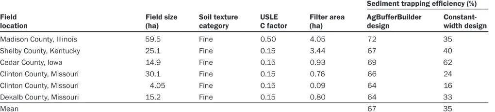
Performance Comparison of Variable and Constant-Width Configurations. Using AgBufferBuilder, several additional fields were analyzed using both the design and the assessment procedures in the same man-ner as shown in figure 3. For each scenario, the design procedure was run first. Then, an assessment was performed on a con-stant-width design having identical total filter area as the designed filter and dis-tributed along portions of margin where the design procedure indicated that a filter would be more effective. The results in every scenario show that the AgBufferBuilder-designed filter would perform better than the constant-width configuration (table 6).

For the scenarios that were analyzed, the AgBufferBuilder-designed filters would trap an average of 67% of the sediments in field runoff during a design storm (61 mm [2.4 in] in one hour) compared to only 35% for con-stant-width filters having the same total area. The degree to which AgBufferBuilder-designed filters outperform constant-width configurations varies widely. Among the test fields, differences ranged from 7% to 48% (table 6). Greater difference would be expected for fields where convergent run-off patterns are more pronounced. Smaller difference would be expected where topog-raphy was more uniform and convergent runoff patterns were less pronounced.

These comparative results indicate better performance by AgBufferBuilder-designed filters than constant-width filters of the same size, often by very large margins. They further indicate that accurately gauging per-formance of filter strips requires accounting for spatially nonuniform patterns of runoff flow from fields.

Limitations of AgBufferBuilder. Planners may prefer to design filter strips for a smaller design storm than is currently modeled in AgBufferBuilder. Some guidance for mak-ing this adjustment is provided in Dosskey et al. (2011) and used in the validation study. However, it has been argued that infre-quent large storms erode and transport the majority of sediment from fields to water-ways, and that conservation practices should be designed for such events (Larson et al. 1997). The current procedures are based on a design storm of 61 mm (2.4 in) in one hour. This size of rainfall event has a 10-year return frequency across the central Plains (e.g., Garden City, Kansas), Corn Belt (e.g., Ames, Iowa), and northern Piedmont (e.g. Durham, North Carolina) (Hershfield 1961). It is more frequent to the south (e.g., a 5-year return for Oklahoma City, Oklahoma; Jackson, Mississippi; Columbus, Georgia; and Fayetteville, North Carolina) and less fre-quent across the northern tier states (e.g., a 25-year return for Minneapolis, Minnesota; Louisville, Kentucky; and Harrisburg, Pennsylvania). Climate change is making such storms increasingly frequent every-where (Walthall et al. 2012).

Topographic information provided in the DEM is central to producing fil-ter designs and performance assessments using AgBufferBuilder. It is assumed that DEMs and flow algorithms accurately

www.swcs.org

70(4):209-217

(8)

Comparison of whole-field average sediment trapping efficiency of AgBufferBuilder-designed and constant-width filter strips having the same total area around a field.

Sediment trapping efficiency (%)

Field Field size Soil texture USLE Filter area AgBufferBuilder Constant-location (ha) category C factor (ha) design width design

Madison County, Illinois 59.5 Fine 0.50 4.05 72 35

Shelby County, Kentucky 25.1 Fine 0.15 3.44 67 40

Cedar County, Iowa 14.9 Fine 0.15 0.93 69 62

Clinton County, Missouri 30.1 Fine 0.15 0.76 66 24

Clinton County, Missouri 4.05 Fine 0.15 0.09 64 16

Dekalb County, Missouri 15.2 Fine 0.15 0.80 64 33

Mean 67 35

Note: USLE C factor = the cover and management factor of the Universal Soil Loss Equation.

reflect patterns on the ground. However, land shaping and drainage modifications that are more recent than when the source elevation data was collected can alter run-off patterns from what would be predicted by the DEM. If those alterations are sub-stantial, AgBufferBuilder results will not accurately represent performance in the field. Therefore, design maps and assessments cre-ated with AgBufferBuilder should be used only after some form of field inspection.

Summary and Conclusions

Sediment trapping effectiveness of con-stant-width filter strips can be greatly limited by spatially nonuniform runoff flow. This result was demonstrated using the GIS-based AgBufferBuilder design and performance assessment tool. The key advancement of this tool is the use of terrain analysis of a DEM for identifying detailed spatial pat-terns of overland runoff to field margins, and then matching filter dimensions to those patterns—larger where there is more runoff, and smaller where there is less. The design procedure produces a filter design that delivers an approximately constant level of sediment trapping efficiency around a field margin. The tool can also estimate the trapping efficiency of existing or other user-defined configurations. Performance estimates using AgBufferBuilder compared closely with measurements on field plots. AgBufferBuilder produces designs that are more effective than constant-width designs where runoff flow from cultivated fields is spatially nonuniform.

Acknowledgements

Funding to support this project was provided by the USDA Forest Service, National Agroforestry Center, Lincoln, Nebraska, and Southern Research Station, Asheville, North

Carolina, to the University of Kentucky (grant no. 10-JV-11330152-119), and from Kentucky state water quality grants (SB-271) administered by the University of Kentucky, College of Agriculture, Lexington, Kentucky. Field data for model validation was provided by a project supported by the Neal Smith National Wildlife Refuge, Iowa State University College of Agriculture and Life Sciences, the Leopold Center for Sustainable Agriculture (SI2009), the USDA’s National Institute of Food and Agriculture (IOW5249) and Sustainable Agriculture Research and Education pro-grams (H001226911), and the US Forest Service Northern Research Station.

References

Daniels, R.B., and J.W. Gilliam. 1996. Sediment and chemical load reduction by grass and riparian filters. Soil Science Society of America Journal 60:246-251. Delgado, J.A., R. Khosla, and T. Mueller. 2011. Recent

advances in precision (target) conservation. Journal of Soil and Water Conservation 66(6):176A-170A. doi:10.2489/jswc.66.6.167A.

Dickey, E.C., and D.H. Vanderholm. 1981. Vegetative filter treatment of livestock feedlot runoff. Journal of Environmental Quality 10:279-284.

Dillaha, T.A., and J.C. Hayes. 1991. A Procedure for the Design of Vegetative Filter Strips. Final Report to the Soil Conservation Service. Washington DC: US Department of Agriculture.

Dillaha, T.A., R.B. Reneau, S. Mostaghimi, and D. Lee. 1989. Vegetative filter strips for agricultural nonpoint source pollution control. Transactions of the American Society of Agricultural Engineers 32:513-519. Dillaha, T.A., J.H. Sherrard, and D. Lee. 1986. Long-term

effectiveness and maintenance of vegetative filter strips. Virginia Water Resources Research Center Bulletin 153. Blacksburg, VA: Virginia Polytechnic Institute and State University.

Dillaha, T.A., J.H. Sherrard, D. Lee, S. Mostaghimi, and V.O. Shanholz. 1988. Evaluation of vegetative filter strips as a best management practice for feed lots. Journal of the American Water Pollution Control Federation 60:1231-1238.

Dosskey, M.G. 2001. Toward quantifying water pollution abatement in response to installing buffers on crop land. Environmental Management. 28:577-598.

Dosskey, M.G., D.E. Eisenhauer, and M.J. Helmers. 2005. Establishing conservation buffers using precision information. Journal of Soil and Water Conservation 60(6):349-354.

Dosskey, M.G., M.J. Helmers, and D.E. Eisenhauer. 2008. A design aid for determining width of filter strips. Journal of Soil and Water Conservation 63(4):232-241. doi:10.2489/jswc.63.4.232.

Dosskey, M.G., M.J. Helmers, and D.E. Eisenhauer. 2011. A design aid for sizing filter strips using buffer area ratio. Journal of Soil and Water Conservation 66(1):29-39. doi:10.2489/jswc.66.1.29.

Dosskey, M.G., M.J. Helmers, D.E. Eisenhauer, T.G. Franti, and K.D. Hoagland. 2002. Assessment of concentrated flow through riparian buffers. Journal of Soil and Water Conservation 57(6):336-343.

Fabis, J., M. Bach, and H.-G. Frede. 1993. Vegetative filter strips in hilly areas of Germany. In Integrated Resource Management & Landscape Modification for Environmental Protection, ed. J.K. Mitchell, 81-88. Proceedings of the International Symposium, Dec. 13, 1993, Chicago, IL. St. Joseph, MI: American Society of Agricultural Engineers.

Flanagan, D.C., G.R. Foster, W.H. Neibling, and J.P. Burt. 1989. Simplified equations for filter strip design. Transactions of the American Society of Agricultural Engineers 32:2001-2007.

Helmers, M.J., D.E. Eisenhauer, M.G. Dosskey, and T.G. Franti. 2002. Modeling Vegetative Filter Performance with VFSMOD. Paper No. MC02-308. St. Joseph, MI: American Society of Agricultural Engineers.

Helmers, M.J., X. Zhou, H. Asbjornsen, R. Kolka, M.D. Tomer, and R.M. Cruse. 2011. Sediment removal by prairie filter strips in row-cropped ephemeral watersheds. Journal of Environmental Quality 41:1531-1539. Hershfield, D.M. 1961. Rainfall Frequency Atlas of the

United States. Technical Paper No. 40. Washington DC: US Weather Bureau.

www.swcs.org

70(4):209-217

(9)

Larson, W.E., M.J. Lindstrom, and T.E. Schumacher. 1997. The role of severe storms in soil erosion: A problem needing consideration. Journal of Soil and Water Conservation 52(2):90-95.

Muñoz-Carpena, R., and J.E. Parsons. 2000. VFSMOD, Vol. 1.04, User’s Manual. Raleigh, NC: North Carolina State University.

Muñoz-Carpena, R., and J.E. Parsons. 2005. VFSMOD-W: Vegetative Filter Strips Hydrology and Sediment Transport Modeling System v.2.x. Homestead, FL: University of Florida. http://carpena.ifas.ufl.edu/vfsmod. Muñoz-Carpena, R., Z. Zajac, and Y.M. Kuo. 2007. Global

sensitivity and uncertainty analysis of the water quality model VFSMOD-W. Transactions of the American Society of Agricultural and Biological Engineers 50:1719-1732.

Nieswand, G.H., R.M. Hordon, T.B. Shelton, B.B. Chavooshian, and S. Blarr. 1990. Buffer strips to protect water supply reservoirs: A model and recommendations. Water Resources Bulletin 26:959-966.

Pankau, R.C., J.E. Schoonover, K.W.J. Williard, and P.J. Edwards. 2012. Concentrated flow paths in riparian buffer zones of Southern Illinois. Agroforestry Systems 84:191-205.

Pike, A., T. Mueller, E. Rienzi, S. Neelakantan, B. Mijatovic. T. Karathanasis, and M. Rodrigues. 2012. Terrain analysis for locating erosion channels: Assessing LiDAR data and flow direction algorithm. In Research on Soil Erosion, ed. D. Godone and S. Stanchi, Chapter 3. InTech Open-Access Books, ISBN: 978-953-51-0839-9, doi: 10.5772/51526.

Suwandono, L., J.E. Parsons, and R. Muñoz-Carpena. 1999. Design Guide for Vegetative Filter Strips using VFSMOD. Paper No. 99-2147. St. Joseph, MI: American Society of Agricultural Engineers.

USDA NRCS (Natural Resources Conservation Service). 2007. Using Revised Universal Soil Loss Equation, Version 2 (RUSLE2) for the Design and Predicted Effectiveness of Vegetative Filter Strips (VFS) for Sediment. Washington DC: US Department of Agriculture.

USDA NRCS. 2013. Filter Strip Code 393. In National Handbook of Conservation Practices. Washington DC: US Department of Agriculture. http://www.nrcs.usda.gov/ Internet/FSE_DOCUMENTS/stelprdb1241319.pdf. Walthall, C.L., J. Hatfield, P. Backlund, L. Lengnick, E.

Marshall, M. Walsh, et al. 2012. Climate change and agriculture in the United States: Effects and adaptation. Technical Bulletin 1935. Washington DC: USDA Agricultural Research Service.

Wischmeier, W.H., and D.D. Smith. 1978. Predicting rainfall erosion losses: A guide to conservation planning. Agriculture Handbook No. 537. Washington DC: US Department of Agriculture. http://topsoil.nserl.purdue. edu/usle/AH_537.pdf.

Wong, S.L., and R.H. McCuen. 1982. The design of vegetative buffer strips for runoff and sediment control.

In Stormwater Management in Coastal Areas, ed. R.H.

McCuen, Appendix J. College Park, MD: University of Maryland Department of Civil Engineering.

Zhou, X., M.J. Helmers, H. Asbjornsen, R. Kolka, and M.D. Tomer. 2010. Perennial filter strips reduce nitrate levels in soil and shallow groundwater after grassland-to-cropland conversion. Journal of Environmental Quality 39:2006-2015.

Zhou, X., M.J. Helmers, H. Asbjornsen, R. Kolka, M.D. Tomer, and R.M. Cruse. 2014. Nutrient removal by prairie filter strips in agricultural landscapes. Journal of Soil and Water Conservation 69(1):54-64. doi:10.2489/ jswc.69.1.54.

www.swcs.org

70(4):209-217