G
T P
,
0
Equilibrium between two solution phases in a binary system
1 2
1 2
1 2
additivitytotal Gibbs energy Gibbs energy of the Gibbs energy of the fist phase second phase
, ,
G n n G n n G n n,
Let us use molar Gibbs energies instead of total Gibbs energies:
2
21 2 1 2 1 2
1 2 1 2
, m m
x x
n n
G n n n n G n n G
n n n n
The total variation of the Gibbs energy is:
1 2 1 2
1 2 1 2
m
m m
G n n G x n n G x
n n G x n n G x
m
(1)
According to the Gibbs criterion of equilibrium, this variation must be non-negative.
Let us understand what is hidden behind Gm
x
and Gm
x .
11 2
m m
dG x x
G x n n
dx n n
2
(2)
Since we know that xn2
n1n2 , it’s straightforward to derive the following expressions for the partial derivatives in (2):
2
2 1 21 1 2 2
, n n
n
x x
n n n n
2
n
2
1
1 2 1 2
n
n n n n
2 (3)
Let us substitute (3) into (2):
2
2 1
1
1 2 1 2
m m
dG n n
G x n n
dx n n n n
2
2 (4)
2
1
12
1 2 1 2
m m
dG n n
G x n n
dx n n n n
2
2 (5)
Substitution of (4) and (5) into (1) gives:
1 2 1 2
1 2 1 2
1 2 1 2
m m
m m
m
G n n G x n n G x
n n G x n n G x
n n G x n n
2
21 2 m
dG n
dx n n
1
1 2
1 2
n n
n n
2
1 2 m 1 2
n
n n G x n n
2
21 2 m
dG n
dx n n
1
1 2
1 2
n n
n n
2
1 2 1 2
1 2 1 2
1
1
m m
m m
n
dG
n n G x x n x n
dx dG
n n G x x n x n
dx
(6)
At first glance, there are 4 variables in (6), but only 2 of them are independent. Why? Because
the number of moles of each component in the system is constant:
(7)
1 1 1, 2 2
nn N nnN2
2
n
It immediately follows from (7) that
1 1 , 2
n n n
(8)
Let us substitute (8) into (6) and rearrange:
1 2 1 2
1 2 1 2
1 2
1
1
1 1
m m
m m
m m m
m m m m
dG
G n n G x x n x n
dx dG
n n G x x n x n
dx
dG dG dG dG
n G x G x n G x G x
dx dx dx dx
m
0
1 1
m m
m m
m m
m m
dG dG
G x G x
dx dx
dG dG
G x G x
dx dx
(9)
We can do two useful things with (9). Firstly, we can rewrite it using the chemical potentials of
components in phases and :
1 1 2 2
0
0
Secondly, the pair of equations (9) can rearranged:
m m
m
m m
dG dG
dx dx
dG
G G x x
dx
Equilibrium among stoichiometric phases in a binary system
Let us consider a reaction involving three stoichiometric solid phases, namely A, B and AB2:
2
A B AB (10)
The total Gibbs energy of the system is composed of the Gibbs energies of individual phases:
2
A B AB
GG G G
Since all phases are stoichiometric ones, their Gibbs energies can be replaced with standard
Gibbs energies, which depend on temperature only:
2
0 0 0
A B AB
GG T G T G T (11)
Now let us use molar quantities and number of moles:
2 2
0 0 0
A A B B AB AB
Gn G T n G T n G T (12)
It may be a bit confusing, but GA0 is used to designate the total Gibbs energy in (11) measured in Joules, while in (12) the same conventional sign is used for the molar Gibbs energy measured in
Joules per mole.
The total variation of the Gibbs energy is:
2 2
0 0 0
A A B B AB A
G n G T n G T n G T
Due to the apparent mass balance conditions
and
2
A AB
n n NA B
2
B 2 AB
n n N (14)
there is only one independent variable in (13). Let such a variable be . Obviously
2
AB
n
2
A AB , B 2
n n n n
2
AB
(15)
Substitution of (15) into (13) results in:
2 2
0 0
AB AB A 2 B
G n G G G
0
(16)
According to the Gibbs criterion of equilibrium, the RHS of (16) must be non-negative:
2 2
0 0 0
AB AB A 2 B
n G G G
0 (17)
Let us realize that is the standard Gibbs energy of reaction
2
0 0
AB A 2 B
G G G
T0
0
rG
0
0
G
0
(10) at the given
temperature, . Let us first realize that it is very unlikely that is equal to zero
exactly. If, however, , then we have a case of the so-called indifferent equilibrium
when neither an extent nor direction of the reaction
0 rG
r
0 rG
2 0
(10) changes the Gibbs energy of the whole
system. What if ? Based on (17), one has to conclude that nAB . Can we interpret this as if a number of moles of must increase? No, it will be a wrong interpretation of what
the Gibbs criterion tells us! We have to say that if the system is in equilibrium, then all possible
processes must result in the increase of the number of moles of , i.e. that in equilibrium is minimal. If , then we conclude that
2
AB
0
0
rG
2
AB
2
AB
n
2
AB 0
n
and that, therefore, all imaginable
processes brining the system out of equilibrium must be accompanied by a decrease of the
number of moles of AB2.
Before clarifying this point graphically, let us write the Gibbs energy of the system in terms of
, and
A
N NB
2
AB
n
(just a reminder: and are the number of moles of A and B.) This can
be achieved by substituting
A
N NB
(14) into (12):
2
22 2
0 0
A AB B AB B AB AB
0 0 0 0 0
AB AB B A B B
2
2
A
A A
G N n G N n G n G
n G G G N G N G
2 2
0
(18)
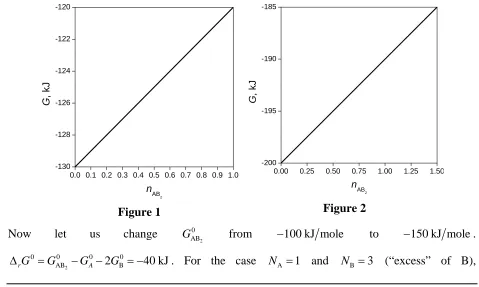
Apparently, (18) is a linear function of . What are the minimal and maximal values of this
variable the Gibbs energy of the system depends upon? No doubts, the minimal value is equal to
2
AB
zero, and . To understand what the upper limit is, let us recall that
and . Consequently, the maximal value is equal to
2
0
AB min A A B B
G n N G N G
B 0 NB2nAB2 0
0
2
A A
N n
A B
min N ,N 2 . If
, then2
AB max
n NA
2 2
0 0
AB max A AB 2 B B B
G n N G G N G0. If
nAB2 max NB 2, then
2
2
0 B 0 0
AB 2 A
G G
AB max
G n A A
2
N N G
.
0
A 70 kJ mole
G ,
For the sake of determinacy, let us use the following quantities:
0
B 20 kJ mole
G
2
0
AB 100 kJ mol
, G e. . Let us consider a
system containing 1 mole of A and 3 moles of B. Apparently,
2
0 0 0 0
AB 2 B 10 k
rG G GA G
J
N 2
min 1,1.5
2
AB max min
n NA, B 1, and
2
AB 1 120J
2
AB 0
n
G n . Verify that
. Refer to
AB2 0
130G n J Figure 1 and realize that equilibrium is achieved at , i.e.
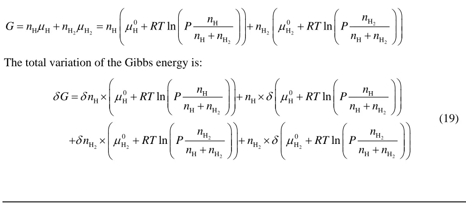
in the point where the total variation of Gibbs energy in not equal to zero, but positive: G0. If NA 2, then
A,NB 2
min 2,1.5
1.52
AB max min
n N
2
AB 1.5 185 J
G n
, ,
. This case is represented in
AB2 0
200G n J Figure 2. Again, only a right-side variation has
a physical sense.
0.0 0.1 -130 -128 -126 -124 -122 -120
0.2 0.3 0.4 0.5 0.6 0.7 0.8 0.9 1.0
G
, kJ
nAB
[image:5.612.64.543.432.719.2]2
Figure 1
0.00 0.25 0.50 0.75 1.00 1.25 1.50 -200
-195 -190 -185
G
, k
J
nAB
2
Figure 2
Now let us change from
2
0 AB
G 100 kJ mole to 150 kJ mole.
. For the case
2
0 0 0 0
AB 2 B 40
rG G GA G
nAB2 max 1, and G n
AB2 1
170 J. G n
AB2 0
130 J0
G
. It is clearly seen from Figure 3
that equilibrium is achieved at and that
2
AB 1
n .
nAB2 max If NA 2 and NB 3 (“excess” of A), then 1.5, and .
. Inspect
AB2 1.5
260 JG n
AB2 0
G n 200J Figure 4 and convince yourself that only the left-side variation has a physical meaning.
0 -170 -160 -150 -140 -130
.0 0.1 0.2 0.3 0.4 0.5 0.6 0.7 0.8 0.9 1.0
G
, kJ
nAB
[image:6.612.68.540.511.720.2]2
Figure 3
0.00 0.25 0.50 0.75 1.00 1.25 1.50 -260
-250 -240 -230 -220 -210 -200
G
, kJ
n
AB2
Figure 4
Equilibrium between two gaseous species
Let us consider a gas-phase reaction 2HH2. The Gibbs energy of the system (at constant
and ) can be written as:
T P
2
2 2 2 2
2 2
H
0 H 0
H H H H H H H H
H H H H
ln
RT P
n ln n
G n n n n RT P
n n n n
The total variation of the Gibbs energy is:
2 2
2 2
2 2 2 2
2 2
0 H 0 H
H H H H
H H H H
H H
0 0
H H H H
H H H H
ln
ln
P
RT P
ln
ln
n n
G n RT n RT P
n n n n
n n
n n RT P
n n n n
2
2 2
2
H H
0 H H
H
H H H H H H H
H H
ln n ln n n n
RT P RT P RT
n n n n n n n
n n
RT
2
H
n
H H
n n
nH2
nH
2
2 H Hn n
2
H
H 2
H H
n n
n n
2
2 2
H
H H H H
H
1
n
RT x n x n
n
(20)
In the same way, the following expression can be derived:
2
2 2 2
2 2
H 0
H
H H H
1
ln n H H H H
RT P RT x n x n
n n n
(21)
Substitution of (20) and (21) into (19) gives:
2
0 H
H H H
H H
ln n
G n RT P n
n n
H
1
RT n
2 2
2
2 2 2
2
H H H H
H 0
H H H
H H
ln
x n x n
n
n RT P n
n n
H2
1
RT n
2 2
2 2 2
H H H H
0 0
H H ln H H H ln H
x n x n
n RT p n RT p
(22)
It should be clear by now that due to the mass balance condition
2
H 2 H
n n NH, there is only one independent variable in (22) and that nH, for instance, can be expressed via
2
H
n
:
2
H 2
n nH
(23)
Substituting (23) into (22) one obtains:
2 2 2 2
2
2 2 2 2
0 0
H H H H H H
H
0 0 2 0
H H H H H H 2
H
2 ln ln
ln 2 ln r ln
G n RT p n RT p
p
n RT p RT p n G RT
p
Since
2
H
n
is an independent variation, the equilibrium is achieved when
2
2 0
H H
ln
p
r K
RT p p G