Sensitivity of African easterly waves to boundary layer conditions

www.ann-geophys.net/26/1355/2008/ © European Geosciences Union 2008

Annales

Geophysicae

Sensitivity of African easterly waves to boundary layer conditions

A. Lenouo1and F. Mkankam Kamga2

1_{Department of Physics, Faculty of Science, University of Douala, P.O. Box 24157 Douala, Cameroon} 2_{LEMAP, Department of Physics, Faculty of Science, University of Yaound´e I, Cameroon}

Received: 27 August 2007 – Revised: 15 February 2008 – Accepted: 13 March 2008 – Published: 11 June 2008

Abstract. A linearized version of the quasi-geostrophic model (QGM) with an explicit Ekman layer and observed static stability parameter and profile of the African easterly jet (AEJ), is used to study the instability properties of the environment of the West African wave disturbances. It is found that the growth rate, the propagation velocity and the structure of the African easterly waves (AEW) can be well simulated. Two different lower boundary conditions are ap-plied. One assumes a lack of vertical gradient of perturbation stream function and the other assumes zero wind perturbation at the surface. The first case gives more realistic results since in the absence of horizontal diffusion, growth rate, phase speed and period have values of 0.5 day−1, 10.83 m s−1and 3.1 day, respectively. The zero wind perturbation at the sur-face case leads to values of these parameters that are 50 per-cent lower. The analysis of the sensitivity to diffusion shows that the magnitude of the growth rate decreases with this pa-rameter. Modelled total relative vorticity has its low level maximum around 900 hPa under no-slip, and 700 hPa under free slip condition.

Keywords. Meteorology and atmospheric dynamics (Cli-matology; Tropical meteorology; Waves and tides)

1 Introduction

It is known that African easterly waves (AEW) are initi-ated and grow mostly over land (Burpee, 1972, 1974; Reed et al., 1977; Mass, 1979; Kwon, 1989; Chang, 1993; Thorn-croft and Hoskins, 1994a; Lenouo et al., 2005; Parker et al., 2005; Hall et al., 2006). These types of waves are nowadays thought to be at the origin of some tropical storms and cy-clones observed in the Western Atlantic and in the Caribbean regions, where they cause enormous damage. The AEW,

Correspondence to: A. Lenouo

([email protected])

which propagates westwards, are synoptic scale atmospheric disturbances that originate in East and Central Africa, where they are observed clearly between June and October (Mass, 1979). It is also known that areas west of the AEW troughs are favorable locations for squall line generation over the entire tropical West Africa (Queney, 1992; Fontaine et al., 1995), and therefore, rainfall in the region is also linked to these disturbances. It has also been suggested that the sea-sonal cycle of AEW strongly influences the development of monsoon in West Africa (Janicot, 2000; Diedhiou et al., 1999; Lenouo, 2004). The detected AEW activity was com-pared with precipitation records in some stations in this re-gion (Taleb and Druyan, 2003).

Quasi-geostrophic models (hereafter QGM) are among the most important approximate formulations for describing the dynamics of easterly waves arising from the mechanism of barotropic-baroclinic instability, as observations suggest (Hall et al., 2006). However, these models do not take into account the effect of vertical motion and of the planetary boundary layer, which is instead parameterized through eddy viscosity (Farrell, 1989). The effect of friction in the bound-ary layer is communicated directly to the free atmosphere through a forced secondary circulation rather than indirectly by the slow process of viscous diffusion (Holton, 1992). In a stably stratified atmosphere, when the forced secondary cir-culation in the lower atmosphere is convergent, there is as-cendance in the cyclonic vortex and this has to be compen-sated by horizontal divergence.

unstable waves is slow in comparison to observation. The growth rates when slip (meaning zero vertical gradient of stream function just above the surface) or no-slip (meaning zero wind perturbation at the surface) boundary conditions are applied in the surface boundary layer, were analysed by Staley (1993). He found that the large cross-isobaric flow of the classic Ekman solution overestimates the damping by a factor of roughly 2. He also found that when a no-slip condition is used, growth rates are significantly reduced, in agreement with Farrell (1989).

It was shown by Thorncroft and Hoskins (1994a) that damping at low levels, when simply mimicking a boundary layer, has very little effect on the normal mode problem. But the influence of damping here was related to the specific jet structure which resulted in stronger growth and larger ampli-tudes at all levels (Thorncroft and Hoskins, 1994b). Mass (1979) linearized the primitive equation model of African waves with boundary layer friction. The inclusion of bound-ary layer dissipation in the lower layer (1000–900 hPa) was by means of a simple Rayleigh dissipation parametrization, but the effect of this particular boundary layer dissipation was not fully discussed. When low-level damping is applied to the momentum and temperature primitive equation model, as in Hall et al. (2006), the wave packet is shifted westward, the surface-intensified section to the east is attenuated more than the rest of the wave, and the upstream/downstream con-trast in tilt and vertical structure is accentuated compared to the undamped modal structure. In Hall et al. (2006), the wave growth is arrested by damping.

The problem examined in this work is the influence of an Ekman damping similar to that of Staley (1993) on the easterly waves in the African lower troposphere. We use the QGM to examine the effects of the average zonal wind vari-ations given by reanalysis data and to study the impact of the effect of an Ekman layer on the properties of the disturbed waves. Specifically, we study the behavior of the characteris-tics and the structure of AEW with an explicit slip or no-slip Ekman layer.

The paper is organized as followed. In Sect. 2, the model and the techniques of eigenanalysis are presented. Then in Sect. 3, details of the data sets, a brief overview of the ba-sic states of the West African atmosphere and results of the eigenanalysis are presented. Discussions and interpretations are also found in this section. Summary and conclusions are in Sect. 4.

2 Theory

As suggested by Burpee (1972), the QGM is adequate to describe the dynamics of AEW arising from barotropic and baroclinic instability. But it has some limitations, as noted by Kwon (1989). For example, the flow at the upper and at the lower levels is quite nongeostrophic (Reed et al., 1977), and cannot be reproduced by the QGM. If we assume the

mean basic flow to be independent of time and zonal coordi-nate, then the undisturbed vorticity vanishes. Hence, a conse-quence of the assumed basic flow is a geostrophic divergence and a vertical velocity in the boundary layer.

The linearized form of the vorticity and of the thermody-namic equations are, respectively:

∂ ∂t(

∂2ψ ∂x2)+U

∂3ψ

∂x3 +(β− ∂2U

∂y2) ∂ψ

∂x =f0 ∂ω ∂p +

K∂ 4_ψ

∂x4 +Km p2 H2

∂2 ∂p2(

∂2ψ

∂x2) (1)

∂ ∂t(

∂ψ ∂p)+U

∂ ∂x(

∂ψ ∂p)−

∂U ∂p

∂ψ ∂x +

σ f0ω=K

∂2 ∂x2(

∂ψ ∂p),(2) whereψ is the streamline function, β the meridional gra-dient of the Coriolis parameter,U the mean zonal velocity, σ=R

p( RT pCp−

∂T

∂p)is the static stability,Rthe specific gas

con-stant,Cp the specific heat capacity at constant pressure,T

the temperature,f0the Coriolis parameter,Kthe horizontal viscosity,Kmthe eddy viscosity,H the height where

verti-cal velocity vanishes,ωthe vertical velocity,pthe pressure, x the zonal coordinate andt the time. The mean wind field is included only through the zonal component, as suggested by the observed dominance of the zonal wind (Mass, 1979). The last term of Eq. (1) represents vertical momentum diffu-sion in the boundary layer and assumesKmand air density

are independent of height. Mean values ofP andH in the boundary layer will be assumed here.

The boundary conditions are given by the values of the vertical wind at the top (PT) and at the bottom (PB) of the

domain. They are such that

ω=0 at P =PT and PB, (3)

wherePT (pressure at the tropopause; see Kwon (1989)) and

PB are 100 and 1000 hPa, respectively. In the lower

atmo-sphere, we take into account the Ekman boundary layer. In the lowest kilometer of the atmosphere, that is the planetary boundary layer, the vertical viscous force is generally com-parable in magnitude to the pressure gradient and Coriolis forces. Thus, the vertical velocity of the classical Ekman pumping is (Holton, 1992)

ω(P0)= −[ρg( Km

2f0) 1/2∂2ψ

∂x2]p0, (4) whereP0=850 hPa is the pressure at the top of the Ekman boundary layer, ρ the density and g the gravitational con-stant. The reduction in growth rate is(Kmf0

2 )

1/2_{/H, where} =1 for the classic Ekman spiral or =2 for half the cross-isobaric flow of the classic Ekman spiral. Typical values of the parameters are as follows (Staley, 1993):Km=5 m2s−1,

f0=10−4s−1, H=10 km and =2, the reduction is 0.068 day−1; forKm=10 m2s−1 andH=10 km, the reduction is

Solutions to Eqs. (1) and (2) are sought in the form of nor-mal modes:

ψ (x, p, t )=9(p)exp[iµ(x−Ct )] (5) and

ω(x, p, t )=(p)exp[iµ(x−Ct )], (6) whereµ=2π/λis the assumed wave number,λis the zonal wavelength; C is the phase velocity,9(p)and(p)are the respective amplitude functions of ψ andω that depend on pressure only. After substituting relations (5) and (6) into Eqs. (1) and (2), the amplitude functions are seen to be gov-erned by the following relations:

Cµ39=µ[µ2U−(β−∂

2_U

∂y2)]9−iµ

4_K9−if0∂ ∂p +

iKmµ2

p2 H2

∂29

∂p2 (7)

Cµ∂9 ∂p =µU

∂9 ∂p −µ

∂U ∂p9−iµ

2_K∂9 ∂p −i

σ

p. (8) By using the central finite difference approximation in the vertical direction, we have:

(_{∂ p}∂)j=

j+1−j−1

1p for oddj and( ∂9 ∂ p)j=

9j+1−9j−1

1p for even

j, where1pis the difference between two consecutive odd (even) pressure levels. The vertical domain has 11 levels in six model layers, where the vorticity equation is written on odd levels and the thermodynamic energy equation on even levels. With these considerations, Eqs. (7) and (8) become: κA9j =Bj9j−i

fo

1P(j+1−j−1)

−iδKmµ 2_p2

H2_(1p)2(9j+2+9j−2−29j) (9) j=1,3,5,7,9 and 11

κ(9j+1−9j−1)=Cj−19j+1−Cj+19j−1+iSjj (10)

j=2,4,6,8 and 10, where κ=C+iµK; A=µ3; Bj=µ[µ2U−(β−d

2_U

dy2)]j; Cj=Uj, Sj=(

σ 1P

µf0 )j and δ=1 in the Ekman layer and 0 above.

In the lowest level9j+2in Eq. (9) corresponds to a point below the ground surface. In that case, the last term is re-placed by

4Kmµ2p2

H2_(1p)2(9j+1+9j−1−29j), (11) where9j+1=912 corresponds to the surface. A boundary condition on912 must be added to the usual condition on ωat the surface, i.e. 912=911, meaning zero vertical gra-dient ofψabove the surface or912=0, meaning zero wind perturbation at the surface. Hence, we can write912=ε911 (ε=1 or 0 for these two cases) and910 can be replaced by (911+99)/2.

Table 1. The numerical values of the parameters (see text for defi-nitions).

Parameters Values

f0 3.7×10−5s−1 β 2.4×10−11m−1s−1

1P 150 hPa

P 900 hPa

H 10 km

g 9.8 m s−2

R 287 m2s−2K−1

Cp 1004 m2s−2K−1

Km 5 m2s−1

After eliminatingfrom Eqs. (9) and (10), we obtain an eigenvalue equation similar to that used by Kwon (1989): κ[P]{X} = [R]{X}, (12) whereκ=Cr+i(Ci−µK)is the optimal eigenvalue,Cr and

Ciare, respectively, the real and the imaginary parts of phase

velocity,{X}eigenvector,[P] and [R] are matrices defined as

follows: {X}=

       91 93 95 97 99 911        ; [P]=       

A−D2 D2 0 0 0 0

D2 F2 D4 0 0 0

0 D4 F4 D6 0 0

0 0 D6 F6 D8 0

0 0 0 D8 F8 D10

0 0 0 0 D10A−D10        and [R]=       

B1−E3,2E1,2 0 0 0 0

E3,2 G3 E3,4 0 0 0

0 E5,4 G5 E5,6 0 0

0 0 E7,6 G7 E7,8 0

0 0 0 E9,8 G9 E9,10

0 0 0 0 E11,10−iγ B11−E9,10−iγ (2ε−3)        ,

where Dj=_Sf0

j1p, Ei,j=CiDj, Fk=A−Dk−Dk−2

(k=2,4,6,8), Gl=Bl−El−2,l−1−El+2,l+1 (l=3,5,7,9) and γ=2Kmµ2p2

H2_(1p)2.

The numerical values of the parameters used in solving Eq. (12) are in Table 1. The vertical velocity at the top of the Ekman layer is given by relation (4).

3 Results and discussion

3.1 Overview of the basic state 3.1.1 Data used

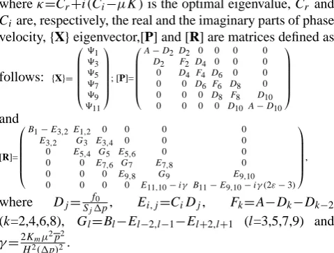
Fig. 1. Spatial variations of mean static stability (in m2s−1Pa−1) over West Africa and Northern Atlantic during summer (JJAS) for the period 1979–2005 at layers (a) 1000–850 hPa, (b) 700–500 hPa and (c) 300–150 hPa. The map of West Africa is depicted as a short dash line. Contour interval for (a) is 2×10−3m2s−1Pa−1, (b) 10−3m2s−1Pa−1and (c) 10−2m2s−1Pa−1.

150 and 50 hPa pressure levels with a spatial resolution of 2.5◦_×2.5◦_{in longitude and latitude, for the summer period}

of June to September (JJAS) of the years 1979 to 2005. The study region is in tropical Africa, from the equator to 30◦N latitude and from 30◦W to 20◦E longitude. It is known that the upper-air temperatures and winds are strongly influenced by observed data in the reanalyses (see Kalnay et al., 1996, for more details).

3.1.2 Measures of static stability parameter

Since earlier observational studies have revealed rather com-plex relations between static stability and the development of convection and precipitations (Randy, 1988), it will be help-ful to briefly analyze the role of static stability measure over West Africa, considered here to vary with pressure. Simply stated, static stability can be regarded as a force resisting up-ward motion in the atmosphere. Thus, it plays a significant role in the control of the vertical motion associated with any atmospheric system (Cortinas and Doswell III, 1997).

Figure 1 shows the spatial pattern of the mean values of this parameter for the period 1979–2005 in the three atmo-spheric layers 1000–850 hPa, 700–500 hPa and 300–150 hPa. We note that, contrary to what is usually assumed (Kwon, 1989), static stability is not vertically constant. As al-ready noted by Jegede and Balogun (1991), it varies spa-tially and seasonally. In the boundary layer (1000–850 hPa), this parameter presents a maximum around 15◦_{N near the}

coasts of Senegal with high values over the continental re-gion (Fig. 1a). In this layer, its gradient is northwards with low values near the equatorial zone and high values in the North over the Sahara. These results are consistent with the stability measure for 1000–850 hPa layer shown by Jegede and Balogun (1991) and based on mean tropospheric sound-ings from eight upper-air stations in West Africa, for an 11-year period (1960–1970). In the 700–500 hPa layer, which is characteristic of free atmosphere, the gradient reverses sign (Fig. 1b) and static stability parameter increases southwards. In the 300–150 hPa layer, the static stability pattern is es-sentially zonal with a positive northward gradient (Fig. 1c). These results show that static stability cannot be considered constant in the tropical troposphere, as admitted by Kwon (1989). In the following study and at any given latitude, we will used the zonal mean vertical profile of static stability computed over the 26-year study period.

3.1.3 Mean zonal vertical wind profile

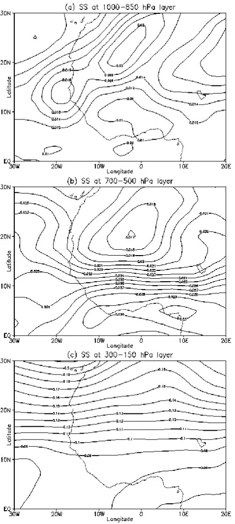
Fig. 2. Observed vertical profile of zonal wind in JJAS season aver-aged over the 1979–2005 period at the AEJ axis (15◦N latitude) at longitudes 5◦W (in long shot dash), 5◦E (in shot dash) at Green-wich meridian (in long shot) and the mean values (in solid). Nega-tive value of zonal wind denote the easterly wind, whereas the pos-itive value is for westerly. AEJ is located here at 600 hPa.

of study. Figure 2 shows these profiles and the mean profile. It would be important to note a few dynamic features of the atmosphere in the region during AEW activity. One notes the presence of westerly wind at the lower atmosphere boundary layer (1000–850 hPa), the AEJ around 600 hPa with a max-imum wind of−12 m s−1, an upper tropospheric jet and the associate vertical shear. In this work, its mean profile con-structed from reanalysis data is used since this zonal wind has all the characteristics of the mean flow used in the AEW simulation.

3.1.4 Analysis of dynamic instabilities

By assuming no horizontal diffusion in the free atmosphere, the quasi-geostrophic potential vorticity (QGPV) gradient equation can be deduced from Eq. (1) as:

∂q ∂y =β−

∂2U

∂y2 −f 2 0

∂ ∂p(

1 σ

∂U

∂p), (13)

whereqis the basic state of quasi-geostrophic vorticity. The first two terms on the right-hand side of this equation are due to horizontal shear (barotropic instability) and the last term is associated with vertical shear (baroclinic instability).

A more comprehensive analysis of the relation between AEJ intensity and AEW activity is made using the Charney

Fig. 3. The quasi-geostrophic potential vorticity gradient at the 600 hPa level averaged from 20◦E to 20◦W for summer 1979–2005 as a function of latitude. Solid line is total QGPV gradient, dash line the baroclinic term and dot line the barotropic term.

and Stern (1962) necessary condition for instability. We used reanalysis data to check the necessary condition for instabil-ity in the area of study. As in Charney and Stern (1962) or Parker et al. (2005), we will assume that the AEJ is an inter-nal jet, the zointer-nal wind is quasi-geostrophic and the monthly means are representative of the instantaneous state of the jet. Using Eq. (13), the QGPV gradient was calculated at the 600 hPa level and averaged from 20◦E to 20◦W for summer 1979–2005. Figure 3 shows the latitudinal variations of the total QGPV gradient, as well as the components barotropic and baroclinic terms. The main condition for instability is met since we note that the QGPV gradient and its two con-tributing terms change sign at around 20◦_{N and 5}◦_{N for}

to-tal and barotropic terms, respectively. However, the QGPV gradient becomes negative in this region, thus implying that the JJAS mean state is dynamically unstable and that the barotropic term also tends to become more dominant. This is in agreement with previous studies in this region (Char-ney, 1973; Thorncroft and Hoskins, 1995; Grist et al., 2002; Parker et al., 2005).

3.2 Characteristics and propagation of normal modes Using the basic states of stability measure and mean wind profile from summer 1979–2005, as calculated in the preced-ing sections from observed data, a normal mode solution to Eq. (12) is sought.

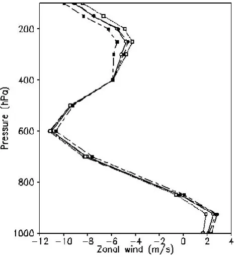
Fig. 4. Growth rate (day−1) as a function of zonal wavelength (km) for (a) ∂ψ_∂p=0 atp=PB(ε=1) and (b)ψ=0 atp=PB(ε=0), and for different values of horizontal diffusion coefficient.

whileτ is close to 3.5 days, implying thatKis of the order of 107m2s−1. Here, a smaller value was used so that the dif-fusion term is about one order of magnitude smaller than the Coriolis term in the vorticity and thermodynamic equations (Chang, 1993).

Figure 4 shows the growth rate of the waves as a function of the zonal wavelength for different values of the horizontal diffusion coefficient, for zero vertical gradient ofψabove the surface (free slip case, Fig. 4a) and zero wind perturbation at the surface (no slip case, Fig. 4b). Growth rates are higher for free slip case. However, they decrease with the horizontal diffusion coefficient in both cases. The wavelength of the most unstable mode is approximately 2900 km, comparable to values observed or simulated by AEW linear models.

We now consider in more detail the results for free slip and no slip conditions. In Fig. 4a (free slip case) the max-imum growth rate is about 0.50 day−1 in the absence of horizontal diffusion. The corresponding period and phase speed are 3.1 day and 10.83 m s−1. Maximum growth rate

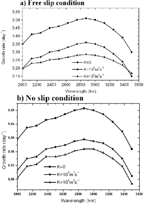
re-Fig. 5. Vertical cross section along 15◦N of the normal mode (λ=2900 km) for (a) slip (ε=1) and (b) no-slip (ε=0) boundary condition forK=0. Solid contour line is total relative vorticity. Ver-tical velocity is also indicated by heavy shading (ascent) and light shading (descent). Contour interval for vorticity is 0.5×10−5s−1.

duces to 0.34 and 0.28 day−1_{when the diffusion coefficient} is 105m2s−1and 106m2s−1, respectively, that is by almost 50 percent. Horizontal diffusion is used to prevent spectral blocking and as a simple sponge to absorb vertically propa-gating planetary wave energy and also to control the strength of the stratospheric winter jets (NCAR Community Atmo-sphere Model (CAM2) reference manual). Its effect has not been sufficiently tested in the modelling of African distur-bances (Chang, 1993) and more analyses are needed in this region.

For the no slip case (Fig. 4b), the wavelength of the most unstable mode remains unchanged but its growth rate is much lower at 0.28 day−1 and its phase speedCr (not shown) is

Thus, the no-slip condition drastically lowers growth rate compared to the free slip condition for the African lower tro-pospheric mode. This is consistent with the results of Far-rell (1989) and Staley (1993), who found that the reduction in growth rate was by 65 to 71 percent in both cases, re-spectively. In the present work, the growth rate reduction in the no-slip condition is 56 percent. For both modes,Cr

(not shown) is in the range of 1 to 2 m s−1, being smaller for the damped case as compared to the undamped. Using basic states corresponding to specific longitudes (5◦W, 5◦E and Greenwich) did not affect the properties of the AEW normal modes, irrespective of the boundary conditions. This is cer-tainly due to the fact that sensitivity to longitudinal variations of the AEJ is negligible, as seen in Fig. 2.

3.3 Structure of the most unstable waves

Considering the case where the fastest-growing mode (λ=2900 km) is associated with the observed average profile of the AEJ in the absence of horizontal diffusion (K=0). Fig-ure 5 shows the vertical structFig-ures of total vorticity and up-ward motion at 15◦N for slip (Fig. 5a) and no-slip (Fig. 5b) boundary conditions.

For the free slip condition, the vorticity field pattern (Fig. 5a) has a gradient which reverses sign at 600 hPa and 250 hPa levels, with the maximum cyclonic vorticity at the lower level. The double reversal of Fig. 5a is a direct conse-quence of the introduction of damping in the boundary layer, since in Thorncroft and Hoskins (1994a), there was no damp-ing and no reversal. This vertical vorticity field has a close resemblance to that of Mass (1979), but differs from the Reed et al. (1977) composite waves, in which the wave trough was located on the maximum of cyclonic vorticity at the lower level.

When the no-slip condition is applied, there are little vis-ible changes in the spatial characteristics of the mode, as shown in Fig. 5b. The magnitude of total vorticity is now reduced by 50 percent, the cyclonic and anticyclonic vortic-ity are now near the boundary layer (900 hPa) and at 400 hPa, respectively. We can also note that they are moving westward and have the same longitudinal separation. The magnitude of vertical velocity is reduced but the spatial pattern remains un-changed. Hence, the total relative vorticity has its low level maximum around 900 hPa under no-slip, and 700 hPa under free slip conditions.

The longititudinal cross section at the same latitude, for the vertical velocityω, are shown in Fig. 5a and b as shaded contours. One notes a region of vertical ascent between the surface and about 350 hPa, located west of the main trough. This ascent maximum is narrower than the descent region, in agreement with the normal mode study by Thorncroft and Hoskins (1994a) or the vertical velocity of the GATE com-posite shown in Reed et al. (1977).

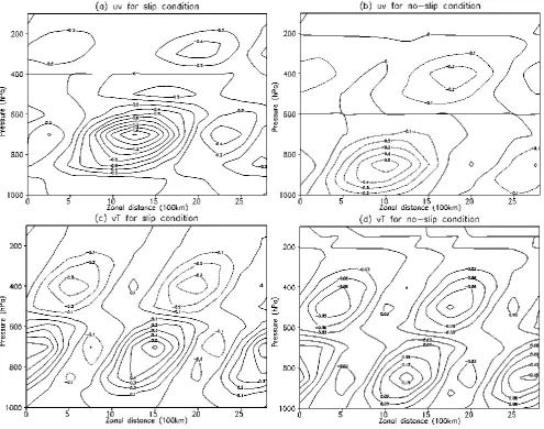
3.4 Eddy fluxes

As in Hall et al. (2006), an assessment of the energetics of AEWs can be obtained from integrated covariances of per-turbation terms. Energy conversions are expressed in terms of second-order momentum departures from mean. Figure 6 shows wave-wave components of northward fluxes of west-erly momentum and temperature associated with slip (Fig. 6a and c) and no-slip (Fig. 6b and d) damped normal mode along 15◦N. When comparing the slip to no-slip mode, a 50 per-cent reduction is noted for easterly flux momentum, whereas meridional temperature flux is reduce by 70 percent. This is in agreement in the slip case from Kiladis et al. (2006). In the lower level, maximum or minimum fluxes are located near 700 hPa and 850 hPa for slip and no-slip conditions, respectively. An easterly wave that grows mainly through barotropic conversions is characterized by essentially hori-zontal easterly momentum fluxes, whereas an easterly wave that grows mainly through baroclinic conversions is charac-terized by meridional temperature fluxes that are mainly ver-tical. The flux divergence of easterly momentum (or con-vergence of westerly momentum) within AEWs varies sub-stantially and slopes northward and upward with height, act-ing to decelerate the easterlies up to around 700 hPa for slip (850 hPa for no-slip) condition. The peak in the flux diver-gence near jet level (700 hPa) is remarkably similar to that of the idealized waves of Hall et al. (2006). The meridional temperature flux shows the expected down gradient trans-port, with a sign reversal at jet level, consistent with baro-clinic growth for the slip or no-slip condition (Fig. 6b and c). Large transports are noted here, reflecting a larger tempera-ture gradient and more baroclinicity at the lower level than at the upper level.

4 Summary and conclusions

We have established here that the lower boundary damping condition is fundamental to the growth rate of the normal-mode of AEW. For an explicit classical Ekman layer where the lower boundary condition assumes ω=0 and there is no vertical gradient of perturbation stream function (ε=1), structure and growth rates are closer to those usually ob-tained, whereas they are significantly reduced when a no-slip condition (ε=0) is used.

Fig. 6. Vertical cross section along 15◦N of wave-wave components of northward fluxes of westerly momentum and temperature associate with the normal mode for (a) and (c) slip (ε=1) and (b) and (d) no-slip (ε=0) boundary condition. Contour intervals for easterly momentum flux are 0.2 m2s−2in (a) and 0.1 m2s−2in (b), and for meridional temperature flux are 0.1 K m s−1in (c) and 0.03 K m s−1in (d).

streamfunction near the surface, but also increases Ekman pumping. The wavelength of the most unstable mode is about 2900 km in both cases. It appears here that the free slip boundary condition gives more realistic results since growth rate, phase speed and period are about 0.5 day−1, 10.83 m s−1_{and 3.1 day, respectively, in the absence of} hor-izontal diffusion, whereas numerical values of wave charac-teristics for no-slip condition are reduced by about 50 per-cent.

The spatial structure of observed AEWs are also well re-produced, especially at the lower level. However, upper level structure is poorly simulated because of the use of the dry mode. Analysis of the instability associated with the hori-zontal and vertical shear of the observed mean flow leads to

the overall conclusion that both the barotropic and baroclinic terms are important, bringing a new perspective to the hy-pothesis that these terms can play a substantial role in wave growth.

Acknowledgements. We are thankful to NOAA-CIRES Climate Di-agnostics Center (Boulder, CO) for providing the NCEP/NCAR Re-analysis data at their Web site at http://www.cdc.noaa.gov. Com-ments by two anonymous reviewers greatly helped to improve the manuscript.

References

Burpee, R. W.: The origin and structure of easterly waves in the lower troposphere of North Africa, J. Atmos. Sci., 29, 77–90, 1972.

Burpee, R. W.: Characteristics of North African easterly waves dur-ing the summer of 1968 and 1969, J. Atmos. Sci., 31, 1556–1570, 1974.

Chang, H.-B.: Impact of desert environment on the genesis of African wave disturbances, J. Atmos. Sci., 50, 2137–2145, 1993. Charney, J. G.: Plametary fluid dynamics, Dynamic Meteorology,

edited by: Morel, P., D. Reidel, 97–352, 1973.

Charney, J. G. and Stern, M. E.: On the instability of internal baro-clinic jets in a rotating atmosphere, J. Atmos. Sci., 19, 159–172, 1962.

Cortinas, J. V. J. and Doswell III, C. A.: Climatology of tropo-spheric static stability across the contiguous United States, Amer. Meteor. Soc., Pre-prints, 16th Conference on Weather Analysis and Forecasting Phoenix, AZ,, 150–152, 1997.

Diedhiou, A., Janicot, S., Vitard, A., de Felice, P., and Laurent, H.: Easterly wave regimes and associated convection over West Africa and tropical Atlantic : results from the NCEP/NCAR and ECMWF reanalyses, Climate Dynamics, 15, 795–822, 1999. Farrell, B. F.: Transient growth of damped baroclinic waves, J.

At-mos. Sci., 42, 2718–2727, 1985.

Farrell, B. F.: Unstable baroclinic modes damped by Ekman dissi-pation., J. Atmos. Sci., 46, 397–401, 1989.

Fontaine, B., Janicot, S., and Moron, V.: ainfall anomaly patterns and wind field signals over West Africa in August (1958–1989), J. Climate, 8, 1503–1510, 1995.

Grist, J. P., Nicholson, S. E., and Barcilon, A. I.: Easterly Waves over Africa: Part II: Observed and Modeled Contrasts between Wet and Dry Years, Mon. Weather Rev., 130, 212–225, 2002. Hall, N. M. J., Kiladis, G. N., and Thorncroft, C. D.:

Three-Dimensional Structure and Dynamics of African Easterly Waves. Part II: Dynamical Modes, J. Atmos. Sci., 63, 2231–2246, 2006. Holton, J. R.: An Introduction to Dynamic Meteorology, 3rd ed.,

Academic Press INC., 591pp, 1992.

Janicot, S.: The West African Monsoon, GBP-WCRP News letter, 11, 6–54, 2000.

Jegede, O. O. and Balogun, E. E.: A contribution of the thermody-namic structure of the atmosphere over continental West Africa : Static stability measure, Atmos. Res., 26, 75–90, 1991. Kalnay, E., Kanamitsu, M., Kistler, R., Collins, W., Deaven, D.,

Gandin, L., Irdell, M., Saha, S., White, G., Woollen, J., Zhu, Y., Chelliah, M., Ebisuzaki, W., Higgins, W., Janowiak, J., Mo, K. C., Ropelewski, C., Wang, J., Leetmaa, A., Reynolds, R., Jenne, R., and Joseph, D.: The NCEP/NCAR 40-year Reanal-ysis Project, B. Am. Meteorol. Soc., 77, 437–471, 1996.

Kiladis, G. N., Thorncroft, C. D., and Hall, N. M. J.: Three-Dimensional Structure and Dynamics of African Easterly Waves. Part I: Observations, J. Atmos. Sci., 63, 2212–2230, 2006. Kwon, H. J.: A re-examination of Genesis of African wave, J.

At-mos. Sci., 46, 3621–3631, 1989.

Lenouo, A.: Impact du param`etre de la stabilit´e statique sur les on-des d’Est africaines, Ph.D. thesis, University of Yaounde I, 2004. Lenouo, A., Mkankam Kamga, F., and Yepdjuo, E.: Weak interac-tion in the African easterly jet, Ann. Geophys., 23, 1637–1643, 2005,

http://www.ann-geophys.net/23/1637/2005/.

Mass, C.: A linear equation model of African wave disturbances, J. Atmos. Sci., 36, 2075–2092, 1979.

Paradis, D., Lafore, J. P., Redelsperger, J. R., and Balaji, V.: African Easterly Waves and Convection. Part I: Linear Simulations, J. Atmos. Sci., 52, 1657–1679, 1995.

Parker, D. J., Thorncroft, C., Burton, R., and Diongue-Niang, A.: Analysis of the African easterly jet, using aircraft observations from the JET2000 experiment, Q. J. Roy. Meteorol. Soc., 131, 1461–1482, 2005.

Queney, P.: El´ements de m´et´eorologie, Masson, 1992.

Randy, A. P.: A review of static stability indices and related ther-modynamic parameters, Illinois State Water Survey, 1988. Reed, R. J., Norquist, D. C., and Recker, E. E.: The structure

and properties of African wave disturbances as observed during phase III of GATE, Mon. Weather Rev., 103, 317–333, 1977. Staley, D. O.: Boundary-Layer Damping of Baroclinic Instability,

J. Atmos. Sci., 50, 772–777, 1993.

Sun, W.: Stability analysis of deep cloud streets, J. Atmos. Sci., 35, 466–483, 1978.

Taleb, E. H. and Druyan, L. M.: Relationships between rainfall and West African wave disturbances in station observations, Int. J. Climatol., 23, 303–313, 2003.

Thorncroft, C. D. and Hoskins, B. J.: An idealized study of African easterly waves. Part 1: A linear view, Q. J. Roy. Meteorol. Soc., 120, 953–982, 1994a.

Thorncroft, C. D. and Hoskins, B. J.: An idealized study of African easterly waves. Part 2: A nonlinear view, Q. J. Roy. Meteorol. Soc., 120, 983–1015, 1994b.