Environmental control of natural gap size distribution in tropical forests

(1)

www.biogeosciences.net/14/353/2017/ doi:10.5194/bg-14-353-2017

Environmental control of natural gap size distribution

in tropical forests

Youven Goulamoussène1, Caroline Bedeau2, Laurent Descroix2, Laurent Linguet1, and Bruno Hérault3

1_{Université de Guyane – UMR Espace-Dev, BP 792, 97337 Cayenne, French Guiana} 2_{Office National des Forêts (ONF), Departement RD, Cayenne, French Guiana}

3_{Cirad, UMR EcoFoG (AgroParisTech, CNRS, Inra, Univ Antilles, Univ Guyane), Kourou, French Guiana}

Correspondence to:Youven Goulamoussène (youven.goulamoussene@ecofog.gf) and Bruno Hérault (bruno.herault@cirad.fr)

Received: 28 July 2016 – Published in Biogeosciences Discuss.: 8 August 2016 Revised: 21 December 2016 – Accepted: 3 January 2017 – Published: 24 January 2017

Abstract.Natural disturbances are the dominant form of for-est regeneration and dynamics in unmanaged tropical forfor-ests. Monitoring the size distribution of treefall gaps is impor-tant to better understand and predict the carbon budget in re-sponse to land use and other global changes. In this study, we model the size frequency distribution of natural canopy gaps with a discrete power law distribution. We use a Bayesian framework to introduce and test, using Monte Carlo Markov chain and Kuo–Mallick algorithms, the effect of local phys-ical environment on gap size distribution. We apply our methodological framework to an original light detecting and ranging dataset in which natural forest gaps were delineated over 30 000 ha of unmanaged forest. We highlight strong links between gap size distribution and environment, primar-ily hydrological conditions and topography, with large gaps being more frequent on floodplains and in wind-exposed areas. In the future, we plan to apply our methodological framework on a larger scale using satellite data. Addition-ally, although gap size distribution variation is clearly under environmental control, variation in gap size distribution in time should be tested against climate variability.

1 Introduction

Natural disturbances caused by forest gaps play an impor-tant role in tropical rainforest dynamics. Canopy gaps caused by the death of one or more trees are the dominant form of forest regeneration because the creation of canopy open-ings continuously reshapes forest structure as gaps are filled

with younger trees (Whitmore, 1989). The first, and per-haps most important, effect of gap occurrence is an imme-diate increase in light intensity (Hubbell et al., 1999), allow-ing sunlight to penetrate the understory. This phenomenon has been widely studied because the opening of gaps con-tributes to the establishment and growth of light-demanding trees (Denslow et al., 1998), thus contributing to the main-tenance of biodiversity. Another effect of canopy gaps is the local modification of the forest nutrient balance (Rüger et al., 2009). When canopy gaps are created, large amounts of dead leaves and wood will be decomposed and mineralized so that the availability of soil nutrients for neighboring trees will increase (Brokaw, 1985). These nutrient patches are also linked to small-scale spatial variations in forest carbon bal-ance, as shown by (Feeley et al., 2007). The relationship be-tween gap formation and the population dynamics of trees or lianas is also quite well understood, with increased liana basal area (Schnitzer et al., 2014) and low-wood-density pi-oneer species that recruit exclusively in newly formed gaps (Molino and Sabatier, 2001).

(2)

and time (Frolking et al., 2009). At high resolution (<10 m), IKONOS satellite images may be well suited for evalu-ating gap dynamics (Espírito-Santo et al., 2014). In French Guiana, the SPOT-4 satellite (20 m spatial resolution) has successfully detected canopy gaps (Colson et al., 2006) us-ing a combination of several spectral bands, such as near and short-wave infrared. However, topographical variation, gap shape, and shade may influence and bias gap detection with optical products. Moreover, persistent cloud cover, which is common in many tropical forests, limits their utility.

Airborne light detecting and ranging (lidar) platforms therefore offer a solution to this problem. Recent develop-ments in lidar have significantly advanced our ability to de-rive accurate measurements of canopy forest structure, to detect gaps, and to assess the effect of spatial and tempo-ral variation on carbon balance (Asner and Mascaro, 2014). (Kellner and Asner, 2009) used remote lidar sensing to quan-tify canopy height and gap size distributions in five tropi-cal rain forest landscapes in Costa Rica and Hawaii. They showed that canopy gaps can be observed with the help of lidar-derived digital canopy models (DCMs) and that gap size frequency distribution (GSFD) can be fit with a power law distribution, suggesting a surprising similarity in canopy gap size frequency distributions on diverse soil types with different geologic substrate ages. (Asner et al., 2013) also used lidar data to analyze whether gap size frequency dis-tribution is modified by topographic and geologic character-istics and again showed that canopy gap size distribution is largely invariant between forests on erosional terra firme and depositional floodplain substrates in the Peruvian Amazon basin. Finally, using airborne lidar, Lobo and Dalling (2014) have recently explored the effect of forest age, topography, and soil type on canopy disturbance patterns across central Panama. For the first time, they highlighted significant effects of slope and of forest age, with a higher frequency of large gaps associated with old-growth forests and gentle slopes.

In the present study, we use a DCM derived from air-borne lidar across a 30 000 ha tropical forest landscape in the Régina forest in French Guiana. This approach provides high-resolution maps of canopy gaps and helps us to under-stand the environmental determinism of gap occurrence in tropical forests. Our specific aims were therefore

– to define canopy gaps from canopy height data using a probabilistic approach;

– to model gap size distribution by inferring a likelihood-explicit discrete power law distribution in a Bayesian framework; and

– to introduce the environment into the scaling parame-ter of the power law distribution and test its predictive ability.

2 Materials and methods

The study site is located in the Régina forest (4◦_{N, 52}◦_W),

where the most common soils are ferralitic. The site is lo-cated on slightly contrasting plateau-type reliefs that are rarely higher than 150 m on average. The forest is typical of French Guianese rainforests. Dominant plant families in the Régina forest include Burseraceae, Mimosoideae, and Caesalpinoideae. The site receives 3806 mm of precipitation per year, with a long dry season from August to mid-November and a short dry season in March (Wagner et al., 2011).

2.1 Data source 2.1.1 Lidar data

Lidar data were acquired by aircraft in 2013 over 30 000 ha of forest by a private contractor, Altoa (http://www.altoa.fr/), using a Riegl LMS-Q560 laser. This system was composed of a scanning laser altimeter with a rotating mirror, a GPS receiver (coupled to a second GPS receiver on the ground), and an inertial measurement unit to record the pitch, roll, and heading of the aircraft. The laser wavelength was near-infrared (from about 800 to 2500 nm). Flights were con-ducted at 500 m above ground level with a ground speed of 180 km h−1, and each flight derived two acquisitions. The li-dar was operated with a scanning angle of 60◦and a 200 kHz pulse repetition frequency. The laser recorded the last re-flected pulse with a precision better than 0.10 m, with a den-sity of 5 pulses m−2.

The DCM was derived from the raw scatter plot consist-ing of the pooled dataset from the two acquisitions. Raw data points were first processed to extract ground points using the TerraScan (TerraSolid, Helsinki) ground routine, which clas-sifies ground points by iteratively building a triangulated sur-face model. Ground points typically made up less than 1 % of the total number of the return pulses. The DCM has a resolu-tion of 1 m. In order to avoid delineating “false” gaps due to river beds, we remove areas very close to natural rivers with a 20 m buffer applied to all shorelines. Additionally, a 25 m buffer was applied to exclude anthropogenic tracks.

2.1.2 Environmental data

We use six environmental variables to synthesize the ob-served environmental gradients. All variables were computed from a lidar digital terrain model (DTM) with 5 m2cells. Slope

(3)

Topographic exposure

We use the TOPographic EXposure (TOPEX) index to measure topographic exposure to wind (Chapman, 2000). TOPEX is a variable that represents the degree of shelter assigned to a location. It was derived from quantitative as-sessment of horizon inclination. The values of this index are closely correlated with the wind-shape index (Mikita and Klimánek, 2012). Exposure is calculated based on the height and distance of the surrounding horizon, which are combined to obtain the inflection angle. We use this angle to quantify topographic exposure (pixel resolution 5 m×5 m). When a large topographic feature, e.g., a mountain, is far off in the distance, the inflection angle is low. When the same mountain is closer, the inflection angle is higher. Therefore, a higher in-flection angle is equal to lower exposure or higher sheltering (Mikita and Klimánek, 2012).

Drained area

Drained area (DA) measures the surface of the hydraulic basin that flows through a cell. A low value indicates that a cell is located at the border between two basins, whereas high values indicate cells located downstream.

Hydraulic altitude

The hydraulic altitude (HA) of each cell, its altitude above the closest stream of its hydraulic basin, was computed from the third-order hydraulic system. Low values, including 0, indicate that the forest plot is potentially temporarily flooded, whereas high values indicate that it is located on a hilltop. Terrain ruggedness index

The terrain ruggedness index (TRI) captures the difference between flat and mountainous landscapes. TRI was calcu-lated using SAGA GIS (SAGA, 2013) as the sum of the alti-tude change between a pixel and its eight neighboring pixels (Riley, 1999).

The height above the nearest drainage

The height above the nearest drainage (HAND) model nor-malizes topography with respect to the drainage network by applying two procedures to the DTM. The initial basis for the HAND model came from the definition of a drainage chan-nel: perennial streamflow occurs at the surface, where the soil substrate is permanently saturated. It follows that the terrain at and around a flowing stream must be permanently satu-rated, independently of the height above sea level at which the channel occurs. Streamflow indicates the localized oc-currence of homogeneously saturated soils across the land-scape. The second basis for the HAND model came from the distinctive physical features of water circulation. Land flows proceed from the land to the sea in two phases: in restrained

flows at the hillslope surface and subsurface, and in freer flows (or discharge) along defined natural channels (Nobre et al., 2011).

2.2 Forest gap definition 2.2.1 Height threshold

To identify discrete canopy gaps, we had to choose a gap threshold height. Some authors define this threshold at 2 m (Brokaw, 1982). (Runkle, 1982) defines a gap as the ground area under a canopy opening that extends to the base of the surrounding canopy trees, these usually being considered to be taller than 10 m, with a trunk diameter at breast height (DBH)>20 cm. However, in practice, defining gap bound-aries is a tricky issue, even in the field. Here, we develop a probabilistic method for detecting canopy gaps from lidar data. We used the DCM to model canopy height distribution considering a mixture distribution of two ecological states: the natural variation of canopy height in mature forests, mod-eled as a normal distribution, and the presence of forest gaps, which lead to a new normal distribution with lower values. We consider that the threshold between the two states is equal to the 0.001th percentile of the height distribution of the canopy; our results appeared robust to the threshold value (see Appendix A). We then define canopy gaps as contiguous pixels (in contact by edges or by vertices) at which the height is less than or equal to the height threshold.

2.2.2 Minimum gap size

In our study, we define the minimum area of a gap asxmin.

We model the gap size frequency distribution with a power law distribution. We use the Pareto distribution in a discrete power law probability density function (Virkar and Clauset, 2014). These distributions have a negative slope and their size frequencies are plotted on a logarithmic scale, allow-ing us to infer the scalallow-ing parameterλ. A value close to 1 means a large number of large gaps. In other words, in forests dominated by small canopy openings, values ofλare larger, whereas smaller values ofλindicate an increased frequency of large gap events (Fisher et al., 2008). In a discrete power law with parameterλ, the probability for gap sizexis given by

p(x)= x

−λ

ζ (xmin, λ)

, (1)

wherexminis the lower truncation point andλis the scaling

parameter.

The statistical analyses were performed in R (R Core Team, 2013), making use of poweRlaw (Clauset et al., 2009) and VGAM (Yee, 2010) packages.

(4)

max-imum distance between the cumulative distribution func-tions (CDFs) of the data and the fitted function (Virkar and Clauset, 2014). We retain, for the remainder of this study, a minimum gap size areaxmin=104 m2, which minimized the

KS distance in our dataset.

2.3 Modeling gap size distribution

Having set the height threshold and minimum gap size, the GSFD is modeled with a discrete Pareto distribution fre-quency.

2.3.1 Model inference

We use a Bayesian framework to estimate model parameters. Here, the value of a parameter is estimated by its posterior distribution, which by definition is proportional to the prod-uct of the likelihood of the model and the parameter prior dis-tribution. The prior distribution is based on prior knowledge of the possible values of a parameter. The posterior densi-ties of the different parameters were estimated using a Monte Carlo Markov chain algorithm (MCMC).

2.3.2 Metropolis–Hastings algorithm

As the model contains many parameters, we built a Metropolis–Hastings (MH) algorithm in which all parame-ters are updated together. Details on the algorithm are given below:

– Y =y1, y2, . . ., ynis the gap size vector;

– X=xg1, xg2, . . ., xgi is the vector of covariates (envi-ronmental variables) for gapg; and

– θ=θ1, θ2, . . ., θiis the model parameter vector. The first values of the parameter vector are initialized as

t=1,θt ∼π_θ0.

For each stept, a new parameter value is sampled from the proposition distribution and a new vector of theta candidates is generated.

θcand∼πprop (2)

Acceptance or rejection of the new candidateθcandis de-termined by computing the likelihood ratio of the two dis-crete Pareto distributions:

ρ(θt, θcand)=L(Y|X, θ

cand₎

L(Y|X, θt₎

| {z }

likelihood

π_θ0(θcand)

π_θ0(θt₎

| {z }

prior

πprop(θt) πprop_(θcand₎

| {z }

proposal

. (3)

The candidateθcandis accepted or rejected as follows:

u∼U[0,1], θcand

θt+1 if u < ρ(θt, θcand),

θt if u > ρ(θt, θcand). (4)

The algorithm is run for 1000 iterations. We use the me-dian of the posterior densities to estimate parameter values, and the distribution of the posterior densities to estimate pa-rameter credibility intervals.

2.3.3 Univariate environmental effects Variable transformation

To improve model inference, parameter significance and in-terpretation, we first transformed some environmental vari-ables:

slope = sqrt(slope) (5)

HAlt = log(HA+1) (6)

TOPEX = |max(TOPEX)−(TOPEX)| (7) The environmental variables are then centered and scaled with R function “scale”.

We first consider each environmental covariate indepen-dently. These covariates are included one-by-one in the model to constrain the exponentλ. We use the exponential function to constrainλ, because the Riemann zeta function only admitsλ >1.

λig=1+exp(θ0+θi×varig), (8)

whereλigis theλvalue dependent on the value of

environ-mental variableiin gapg,θ0 is the intercept, andθi quan-tifies the effect of covariates var on the gap size distribution varig.

2.3.4 Multivariate model Principal component analysis

We first investigated the collinearity of environmental data through principal component analysis (PCA) of the normal-ized environmental dataset.

Model

To build the final model, we used the results of the univariate model (Table 1) and the PCA (Fig. 2) and set

λ=1+exp(θ0+θ1×Slope+θ2×TOPEX

+θ3×HAlt+θ4×HAND). (9)

Variable selection

(5)

Canopy height (m)

Density

0 10 20 30 40 50 60

0.00

0.01

0.02

0.03

0.04

0.05

Canopy height

[image:5.612.162.442.68.369.2]

Natural variation of canopy height Presence of low height in canopy height

Figure 1.Canopy height distribution. Canopy height considered as a mixture distribution of two ecological features. The first (blue curve) is the natural variation in canopy height, modeled as a normal distribution. The second (red curve) is linked to the presence of low heights in the total canopy height distribution, likely to be due to a forest gap. We set the gap threshold to the 0.001th percentile of the blue curve density, i.e., 11 m.

Table 1.List of environmental variables, abbreviations, units, and values of the posteriors in univariate models.

Parameter Abbreviation Unit Posterior value Confidence interval (CI 95%)

Slope Slope ◦ 0.0735 [−0.02; 0.15]

Terrain ruggedness index TRI – 0.0718 [0.04; 0.10]

TOPographic EXposure TOPEX – −0.082 [−0.12;−0.05]

Drained area DA m2 −0.0176 [−0.09; 0.05]

The hydraulic altitude HA m −0.0177 [−0.05; 0.02]

HAND HAND – −0.003 [−0.08; 0.09]

the MH and KM algorithms to estimate the indicatorsI and infer their a posteriori distribution in addition toθ.

We start the KM algorithm with t=1, θt∼π_θ0, I_jt∼

Ber(0.5)for j =1, . . ., i. For each covariate j (selected in random order), we use the MH algorithm to update θj. To updateIj, we compute the ratioρ(Eq. 10) and generateIjt+1 from a Bernoulli distributionBern(ρ):

ρ= 1

1+L(Y|eX,θ

t_,I

j=0,I−tj)

L(Y|eX,θt,Ij=1,I−tj)

. (10)

[image:5.612.136.458.456.567.2]

(6)

[image:6.612.312.546.63.323.2]

Figure 2.Results of the principal component analysis of the envi-ronmental variables.

3 Results

3.1 Gap delineation

In this study, we used a forest canopy height mixture model to define the maximum height of a given pixel to be included in a forest gap. This probabilistic method produced results that fit the observed canopy height distribution. We retained the 11 m threshold that corresponds to the 0.001th percentile of the canopy height distribution (Fig. 1). Given this height, we retained the surface xmin=104 m2 that minimized the

KS distance between predictions and observations. Here, our gap definition was therefore defined as an area>104 m2, in which the lidar measured canopy height is always≤11 m. 3.2 Basic statistics

We mapped 12 293 gaps with vegetation ≤11 m in height. The mean gap size was 236 m2with a minimum gap size of 104 m2and a maximum of 29 063 m2. The total gap area was about 290 ha, or 1 % of the whole surveyed area. The ob-served gap size distribution was modeled with a Pareto dis-tribution (Fig. 3), leading to a scaling parameterλxminof 2.6. 3.3 Univariate models

All variables had an effect on gap size distribution (Table 1). The scaling coefficientλis related to the ratio of small gaps to large gaps, with values close to 1 indicating a higher

fre-● ● ●●● ● ●●_●●● ●_● ● ● ● ● ● ● ● ●●●●● ●● ● ● ● ●_●● ● ● ● ● ● ● ● ● ● ●●_●● ● ●● ● ● ● ● ● ●● ● ●● ● ●● ● ● ● ● ● ●●● ● ● ● ● ● ● ● ● ● ● ● ● ● ● ● ● ● ● ● ● ● ● ● ● ● ● ● ● ● ● ● ● ● ● ● ● ● ● ●●● ● ● ● ● ● ● ● ● ● ● ● ● ● ● ● ● ● ● ● ● ● ● ● ● ● ● ● ● ● ●● ● ● ● ● ● ● ● ● ● ● ● ● ● ● ● ● ● ● ● ● ● ● ● ● ● ● ● ● ● ● ● ● ● ● ● ● ● ● ● ●● ● ● ● ● ● ● ● ● ● ● ● ● ● ● ● ● ●● ● ● ● ● ● ● ● ● ● ● ● ● ● ● ● ● ●● ● ● ● ● ● ● ● ● ● ● ● ● ● ● ● ● ● ● ● ● ● ● ● ● ● ● ● ● ● ● ● ● ● ● ● ● ● ● ● ● ● ● ● ● ● ● ●● ● ● ● ● ● ● ● ● ● ● ● ● ● ●● ● ● ● ● ● ● ● ● ● ● ● ● ● ● ● ● ● ● ● ● ● ● ● ● ● ● ● ● ● ● ● ● ● ● ● ● ● ● ● ● ● ● ● ● ● ● ● ● ● ● ● ● ● ● ● ● ● ● ● ● ● ● ● ● ● ● ● ● ● ● ● ● ● ● ● ● ● ● ● ● ● ● ● ● ● ● ● ● ● ● ● ● ● ● ● ● ● ● ● ● ● ● ● ● ● ● ● ● ● ●● ● ● ● ● ● ● ● ● ● ● ● ● ● ● ● ● ● ● ● ● ● ● ● ● ● ● ● ● ● ● ● ● ● ● ● ● ● ● ● ● ● ● ● ● ● ● ● ● ● ● ● ● ● ● ● ● ● ● ● ● ● ● ● ● ● ● ● ● ● ● ● ●●● ● ● ● ● ● ● ● ● ● ● ● ● ● ● ● ● ● ● ● ● ● ● ● ● ● ● ● ● ● ● ● ● ● ● ● ● ● ● ● ● ● ● ● ● ● ● ● ● ● ● ● ● ● ● ● ● ● ● ● ● ● ● ● ● ● ● ●● ● ● ● ● ● ● ● ●●● ● ● ● ● ● ●●●●● ● ● ● ● ● ●●● ● ● ● ● ● ● ●●●●●● ● ● ● ● ● ● ● ● ● ● ● ● ● ● ● ● ●●● ● ● ● ● ● ● ● ● ● ● ● ● ● ● ● ● ● ● ● ● ● ● ● ● ● ●●●●●●● ● ● ● ● ● ● ● ● ● ● ● ● ● ● ● ● ● ● ● ● ● ● ● ● ● ● ● ●●●●●●● ● ● ● ● ● ●●●●●●●● ● ●●● ● ● ● ● ● ●●●●●●●●●●●●●●●●●●●●●●●●●● ● ●●●●●●●● ● ●●●●●●●●●●●●●●●●●●●●●●●●●●●●●● ● ● ●●●●●● ● ● ●●●●●●●●●●●●●●●●●●●●●●●●●●●●●●●●●●●●●●●●●● ●●●●●●●●●●●●●●●●●●●●● ●● ●● ● ●

Gap size m2

Frequency 1 2 5 10 20 50 100 200

100 200 500 1000 2000 5000 10 000

Figure 3.The observed gap size frequency distributions modeled as a power law function withλ=2.6.

quency of large gaps and vice versa. Parameter estimates for slope and TRI show high occurrence of small gaps for large values of the two variables. Contrarily, the effects of DA, HAND, HAlt, and TOPEX onλare clearly negative, mean-ing that the frequency of large gaps increases with large val-ues.

3.4 The multivariate model

To define the final multivariate predictive model, we used the significant results of the univariate models together with the output of the PCA, in order to avoid multicollinearity. 3.4.1 Variable selection

[image:6.612.52.286.66.328.2]

(7)

HAlt

Slope

TOPEX

HAND

Acceptance rate

[image:7.612.66.263.65.280.2]

0.0 0.2 0.4 0.6 0.8 1.0

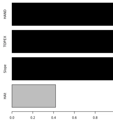
Figure 4.Results of the Kuo–Mallick algorithm for variable selec-tion. Variables were included in the final model when their value was close to 100 %: slope, TOPEX and HAND.

Environmental covariates with posterior KM values close to 1, namely slope, TOPEX, and HAND (Eq. 9), were re-tained in the final model (Fig. 4). Parameter estimates of the final model indicated that the greatest effects on gap size dis-tribution were caused by TOPEX and HAND.

4 Discussion 4.1 Methodology 4.1.1 Gap detection

Delineating forest gaps is a persistent challenge for foresters and ecologists, among whom Brokaw’s gap definition (1982) has remained extensively used, in which “a ‘hole’ in the for-est extending through all levels down to an average height of 2 m above the ground,” must be defined by an experienced observer. There are several studies that do not use this 2 m threshold definition of gaps, but instead 10 m (e.g., Hubbell et al., 1999; van der Meer and Bongers, 1996; Welden et al., 1991). However, in this study we have decided to use a prob-abilistic approach, modeling height distribution as a mixture of two normal laws. We found a height, 11 m, which is much higher than that in Brokaw’s definition but is consistent with our field experience, where woody debris, dead canopy tree boles, and residual saplings (i.e., remnants that survive the gap formation event) may rise well above 2 m. For example, (Hubbell et al., 1999) showed that small stems frequently remained in gaps up to 4–5 m in height, while (Lieberman et al., 1985) reported broken and damaged stems up to 10 m tall within a gap. The choice of the values of height and

threshold may be adapted to different forest types and to-pographic characteristics. In our case, the choice was fully data-driven using the DCM and the digital elevation model (DEM) and no ecological knowledge. Within our framework it is likely that in waterlogged areas, areas covered with ma-ture trees that do not exceed the height thresholds may ap-pear in our analysis as forest gaps. In order to clarify this question, an approach using time series would allow us to identify these “false” gaps that never get filled and thus are not part of the forest endogeneous dynamics. These are not gaps in the ecological meaning.

Defining minimum gap size is also a delicate proposition. Some authors, working with high-definition lidar data, have considered a minimum gap size (xmin) of 1 m2(Asner et al.,

2013; Kellner and Asner, 2009). This minimum gap size is unrealistic from an ecological perspective given that a hole of several square meters in the canopy may simply reflect the distance between two crowns. Brokaw recommended a range from 20 to 40 m2 based on his field experience. We have worked with a minimum gap size of 104 m2, and based this value on the minimized Kolmogorov–Smirnov distance between observed and predicted values.

We built on previous studies that show that gap size distri-bution follows a power law distridistri-bution. However, the under-lying mechanisms that control this distribution are still un-clear. The Bayesian framework we developed allowed us to detail the contributions of each environmental variable to the size of each individual gap. Because the precise environmen-tal variables were explicitly taken into account in the model likelihood of each gap, we were able to predict gap size dis-tribution from environmental covariates, a difficult task when the scale exponent is estimated once, at the forest level, and compared between forests. The global scale exponent that we estimated for an average environment (λ=2.6) is con-sistent with some previous studies (Kellner and Asner, 2009; Kellner et al., 2011), though slightly larger than those of oth-ers: (Lobo and Dalling, 2014), [1.97; 2.15], and (Asner et al., 2013), [1.70; 2.03].

4.2 Environmental effects on gap size frequency distribution

For the first time, gap size distribution integrates environ-mental variables as a linear combination of the scale parame-ter (λ) of a discrete Pareto distribution frequency. Our results suggest that three covariates drive the gap size frequency dis-tribution in our forest: slope, HAND, and TOPEX (Fig. 5). 4.2.1 Slope

(8)

counter-0.48

0.50

0.52

θInt

0.48

0.50

0.52

density(result[, i])$y

density(result[, i])$x

−0.01

0.01

0.03

θSlope

−0.01

0.01

0.03

−0.08

−0.05

−0.02

θTOPEX

−0.08

−0.05

−0.02

−0.03

−0.01

0.01

θHAND

Chain index

0 200 400 600 800 1000

−0.03

−0.01

0.01

[image:8.612.107.497.69.344.2]

Density

Figure 5.Posterior distribution of the environmental variables in the final multivariate model.

intuitive at first, as treefall may be (i) more prone to inducing cascading effects when slopes are steep and (ii) more fre-quent in slopes where soils are shallow with lateral drainage (Gourlet-Fleury et al., 2004), impeding deep rooting of trees. However, the forest turnover is more important in bottom-lands where slopes are gentle (Durrieu de Madron, 1994). Considering that large gaps may be created solely by contigu-ous and independent treefalls, larger gaps may then be ex-pected in bottomlands from a purely probabilistic approach. And given the positive link between wood density and steep slopes (Ferry et al., 2010), trees may be more resistant to cas-cading effects than they are in bottomlands.

4.2.2 Water saturation

HAND is a binary variable that takes the value 1 on water-saturated soils. Becauseλdecreases when HAND equals 1, the frequency of large gaps increases in floodplains and bot-tomlands. These results support the findings of (Korning and Balslev, 1994), highlighting more dynamic forests in flood-plains subject to large flooding events that lead to cascad-ing treefall events. Together with Asner et al. (2013), our results suggest that we can effectively extend these results to bottomlands, where we already know that aboveground biomass and mean wood density are 10 % lower than on hill-tops (Ferry et al., 2010). Given its ease of implementation on a land-surface model and its high predictive power, HAND

covariates present great potential applicability for gap size distribution prediction.

4.2.3 Topographic exposure

(9)

5 Conclusions

To our knowledge, this is the first study where the precise environmental descriptors associated with each canopy gap were explicitly taken into account in the calculation of the model likelihood. We were able to do so because we wrote the general model likelihood as the product of all the single likelihoods (i.e., each gap had its own likelihood depending on the environmental covariate values). Doing so, we were able to predict gap size distribution from the fine environ-mental covariates, an impractical task when the scale expo-nent is estimated once at the forest level (i.e., mixing all the found gaps together) and compared between forests a poste-riori. We also put forward an innovative method to define a height threshold and minimum gap size using two probabilis-tic approaches. The modeled distribution of canopy height as a mixture of two distributions provides a clear height thresh-old, while the minimization of KS distance between observed and predicted data proves to be efficient for setting the min-imum gap size. We use a Bayesian framework in which the

model likelihood of each gap is expressed as a function of the unique environment local to the gap, highlighting the pre-dominant role of the topographic exposure and waterlogging in determining gap size distribution. We expected that slope would also play an important role, with steeper slopes lead-ing to larger gap sizes. However, we found that a steeper slope led to smaller gaps, as already highlighted by (Lobo and Dalling, 2014). We suggest that our modeling approach can be a basis for the development of large-scale methodolo-gies using satellite data to understand gap-phase dynamics at a regional scale, combining lidar and radar remote sensing tools.

6 Data availability

(10)

[image:10.612.130.465.133.246.2]

Appendix A

Table A1.List of environmental variables, abbreviations, units, and values of the posteriors in univariate models for a height threshold equal to the 0.0001th percentile of the height distribution of the canopy.

Parameter Abbreviation Unit Posterior value Confidence interval (CI 95 %)

Slope Slope ◦ 0.119 [0.0416; 0.208]

TOPographic EXposure TOPEX – −0.128 [−0.188; 0.00202]

Drained area DA m2 0.0843 [−0.0574; 0.179]

The hydraulic altitude HAlt m −0.0135 [−0.04; 0.042]

[image:10.612.138.459.305.416.2]

HAND HAND – −0.0615 [−0.152; 0.0162]

Slope Slope ◦ 0.0735 [−0.02; 0.15]

Drained area DA m2 −0.0176 [−0.09; 0.05]

The hydraulic altitude HAlt m −0.0177 [−0.05; 0.02]

HAND HAND – −0.003 [−0.08; 0.09]

Slope Slope ◦ 0.0975 [−0.02; 0.17]

Drained area DA m2 −0.004 [−0.08; 0.05]

The hydraulic altitude HAlt m 0.063 [−0.04 ; 0.08]

[image:10.612.139.458.475.587.2]

(11)

Competing interests. The authors declare that they have no conflict of interest.

Acknowledgements. We thank the handling editor, Ervan

Rutishauser and Marijn Bauters for their thoughtful comments on a previous version of this paper. This study is part of the GFclim project funded by PO-Feder Région Guyane. Bruno Hérault was supported by a grant from the Investing for the Future program (managed by the 350 French National Research Agency – ANR, labex CEBA, ref. ANR-10-LABX-0025).

Edited by: A. Rammig

Reviewed by: E. Rutishauser and M. Bauters

References

Asner, G. P. and Mascaro, J.: Mapping tropical forest carbon: Cal-ibrating plot estimates to a simple LiDAR metric, Remote Sens. Environ., 140, 614–624, doi:10.1016/j.rse.2013.09.023, 2014. Asner, G. P., Kellner, J. R., Kennedy-Bowdoin, T., Knapp, D. E.,

Anderson, C., and Martin, R. E.: Forest canopy gap distribu-tions in the southern Peruvian Amazon, PloS one, 8, e60875, doi:10.1371/journal.pone.0060875, 2013.

Bianchini, E., Garcia, C. C., Pimenta, J. A., and Torezan, J.: Slope variation and population structure of tree species from different ecological groups in South Brazil, An. Acad. Bras. Ciênc., 82, 643–652, 2010.

Bicknell, J. E., Phelps, S. P., Davies, R. G., Mann, D. J., Struebig, M. J., and Davies, Z. G.: Dung beetles as indicators for rapid im-pact assessments: evaluating best practice forestry in the neotrop-ics, Ecol. Indic., 43, 154–161, 2014.

Brokaw, N. V.: The definition of treefall gap and its effect on mea-sures of forest dynamics, Biotropica, 14, 158–160, 1982. Brokaw, N. V.: Gap-phase regeneration in a tropical forest, Ecology,

66, 682–687, 1985.

Chapman, L.: Assessing topographic exposure, Meteorol. Appl., 7, 335–340, 2000.

Clauset, A., Shalizi, C. R., and Newman, M. E.: Power-law distri-butions in empirical data, SIAM Rev., 51, 661–703, 2009. Colson, F., Gond, V., Freycon, V., Bogaert, J., and Ceulemans, R.:

Detecting natural canopy gaps in Amazonian rainforest, Bois et forêts des tropiques, 289, 69–79, 2006.

Denslow, J. S., Ellison, A. M., and Sanford, R. E.: Treefall gap size effects on above-and below-ground processes in a tropical wet forest, J. Ecol., 86, 597–609, 1998.

Durrieu de Madron, L.: Mortalité des arbres en forêt primaire de Guyane française, Bois et forêts des tropiques, 239, 43–57, 1994. Espírito-Santo, F. D., Keller, M. M., Linder, E., Oliveira Junior, R. C., Pereira, C., and Oliveira, C. G.: Gap formation and car-bon cycling in the Brazilian Amazon: measurement using high-resolution optical remote sensing and studies in large forest plots, Plant Ecol. & Divers., 7, 305–318, 2014.

Feeley, K. J., Davies, S. J., Ashton, P. S., Bunyavejchewin, S., Nur Supardi, M., Kassim, A. R., Tan, S., and Chave, J.: The role of gap phase processes in the biomass dynamics of tropical forests, P. Roy. Soc. Lond. B Bio., 274, 2857–2864, doi:10.1098/rspb.2007.0954, 2007.

Ferry, B., Morneau, F., Bontemps, J.-D., Blanc, L., and Freycon, V.: Higher treefall rates on slopes and waterlogged soils result in lower stand biomass and productivity in a tropical rain forest, J. Ecol., 98, 106–116, 2010.

Fisher, J. I., Hurtt, G. C., Thomas, R. Q., and Chambers, J. Q.: Clus-tered disturbances lead to bias in large-scale estimates based on forest sample plots, Ecol. Lett., 11, 554–563, 2008.

Frolking, S., Palace, M. W., Clark, D., Chambers, J. Q., Shugart, H., and Hurtt, G. C.: Forest disturbance and recovery: A general review in the context of spaceborne remote sensing of impacts on aboveground biomass and canopy structure, J. Geophys. Res.-Biogeo., 114, G00E02, doi:10.1029/2008JG000911, 2009. Gourlet-Fleury, S., Guehl, J.-M., and Laroussinie, O.: Ecology

and management of a neotropical rainforest. Lessons drawn from Paracou, a long-term experimental research site in French Guiana, edited by: Gourlet-Fleury, S., Guehl, J. M., and Laroussinie, O., Elsevier, Paris, France, 326 pp., 2004.

Guitet, S., Cornu, F., Brunaux, O., Betbeder, J., Carozza, J.-M., and Richard-Hansen, C.: Landform and landscape mapping, French Guiana (South America), Journal of Maps, 9, 325–335, 2013.

Hubbell, S. P., Foster, R. B., O’Brien, S. T., Harms, K., Condit, R., Wechsler, B., Wright, S. J., and De Lao, S. L.: Light-gap distur-bances, recruitment limitation, and tree diversity in a neotropical forest, Science, 283, 554–557, 1999.

Kellner, J. R. and Asner, G. P.: Convergent structural responses of tropical forests to diverse disturbance regimes, Ecol. Lett., 12, 887–897, 2009.

Kellner, J. R., Asner, G. P., Vitousek, P. M., Tweiten, M. A., Hotchkiss, S., and Chadwick, O. A.: Dependence of forest struc-ture and dynamics on substrate age and ecosystem development, Ecosystems, 14, 1156–1167, 2011.

Korning, J. and Balslev, H.: Growth and mortality of trees in Ama-zonian tropical rain forest in Ecuador, J. Veg. Sci., 5, 77–86, 1994.

Kuo, L. and Mallick, B.: Variable Selection for Regression Mod-els, The Indian Journal of Statistics, Series B (1960–2002) 60, Bayesian Analysis (Apr. 1998), 65–81, published by: Indian Sta-tistical Institute Stable, available at: http://www.jstor.org/stable/ 25053023 (last access: 23 January 2017), 1998.

Lieberman, D., Lieberman, M., Peralta, R., and Hartshorn, G. S.: Mortality patterns and stand turnover rates in a wet tropical forest in Costa Rica, J. Ecol., 73, 915–924, 1985.

Lloyd, J., Gloor, E. U., and Lewis, S. L.: Are the dynam-ics of tropical forests dominated by large and rare distur-bance events?, Ecol. Lett., 12, E19–E21, doi:10.1111/j.1461-0248.2009.01326.x, 2009.

Lobo, E. and Dalling, J. W.: Spatial scale and sampling reso-lution affect measures of gap disturbance in a lowland trop-ical forest: implications for understanding forest regeneration and carbon storage, P. Roy. Soc. Lond. B Bio., 281, 20133218, doi:10.1098/rspb.2013.3218, 2014.

Mikita, T. and Klimánek, M.: Topographic Exposure and its Practi-cal Applications, Landscape Ecol., 3, 42–51, 2012.

(12)

Negrón-Juárez, R. I., Chambers, J. Q., Hurtt, G. C., Annane, B., Cocke, S., Powell, M., Stott, M., Goosem, S., Metcalfe, D. J., and Saatchi, S. S.: Remote Sensing Assessment of Forest Disturbance across Complex Mountainous Terrain: The Pattern and Severity of Impacts of Tropical Cyclone Yasi on Australian Rainforests, Remote Sensing, 6, 5633–5649, 2014.

Nelson, B. W., Kapos, V., Adams, J. B., Oliveira, W. J., and Braun, O. P.: Forest disturbance by large blowdowns in the Brazilian Amazon, Ecology, 75, 853–858, 1994.

Nobre, A., Cuartas, L., Hodnett, M., Rennó, C., Rodrigues, G., Sil-veira, A., Waterloo, M., and Saleska, S.: Height above the nearest drainage–a hydrologically relevant new terrain model, J. Hydrol., 404, 13–29, 2011.

Puerta-Piñero, C., Muller-Landau, H. C., Calderón, O., and Wright, S. J.: Seed arrival in tropical forest tree fall gaps, Ecology, 94, 1552–1562, 2013.

R Core Team: R: A language and environment for statistical com-puting, available at: http://www.R-project.org (last access: 21 January 2017), 2013.

Riley, S. J.: Index That Quantifies Topographic Heterogeneity, In-termountain Journal of Sciences, 5, 23–27, 1999.

Rüger, N., Huth, A., Hubbell, S. P., and Condit, R.: Response of re-cruitment to light availability across a tropical lowland rain forest community, J. Ecol., 97, 1360–1368, 2009.

Runkle, J. R.: Patterns of disturbance in some old-growth mesic forests of eastern North America, Ecology, 63, 1533–1546, 1982. SAGA, G.: System for automated geoscientific analyses, avail-able at: www.saga-gis.org/en/index.html (last access: 21 January 2017), 2013.

Schnitzer, S. A., van der Heijden, G., Mascaro, J., and Carson, W. P.: Lianas in gaps reduce carbon accumulation in a tropical forest, Ecology, 95, 3008–3017, 2014.

van der Meer, P. J. and Bongers, F.: Formation and closure of canopy gaps in the rain forest at Nouragues, French Guiana 1996, 126, 167–179, doi:10.1007/BF00045602,blackboxCheck., 1996. Virkar, Y. and Clauset, A.: Power-law distributions in binned

em-pirical data, Ann. Appl. Stat., 8, 89–119, 2014.

Wagner, F., Hérault, B., Stahl, C., Bonal, D., and Rossi, V.: Mod-eling water availability for trees in tropical forests, Agr. Forest Meteorol., 151, 1202–1213, 2011.

Welden, C. W., Hewett, S. W., Hubbell, S. P., and Foster, R. B.: Sapling Survival, Growth, and Recruitment: Relationship to Canopy Height in a Neotropical Forest, Ecology, 72, 35–50, doi:10.2307/1938900, 1991.

Whitmore, T.: Canopy gaps and the two major groups of forest trees, Ecology, 70, 536–538, 1989.