Ann. Geophys., 28, 327–337, 2010 www.ann-geophys.net/28/327/2010/
© Author(s) 2010. This work is distributed under the Creative Commons Attribution 3.0 License.
Annales
Geophysicae
Density enhancements associated with equatorial spread
F
J. Krall1, J. D. Huba1, G. Joyce2, and T. Yokoyama3
1Plasma Physics Division, Naval Research Laboratory, Code 6790, 4555 Overlook Ave., SW, Washington, D.C.,
20375-5000, USA
2Icarus Research, Inc., P.O. Box 30780, Bethesda, MD 20824-0780, USA
3Department of Earth and Atmospheric Sciences, Cornell University, Ithaca, NY, 14850, USA
Received: 4 September 2009 – Revised: 17 November 2009 – Accepted: 23 November 2009 – Published: 1 February 2010
Abstract. Forces governing the three-dimensional structure of equatorial spread-F (ESF) plumes are examined using the NRL SAMI3/ESF three-dimensional simulation code. As is the case with the equatorial ionization anomaly (IA), density crests within the plume occur where gravitational and dif-fusive forces are in balance. LargeE×Bdrifts within the ESF plume place these crests on field lines with apex heights higher than those of the background IA crests. Large pole-ward field-aligned ion velocities within the plume result in large ion-neutral diffusive forces that support these ioniza-tion crests at altitudes higher than background IA crest al-titudes. We show examples in which density enhancements associated with ESF, also called “plasma blobs,” can occur within an ESF plume on density-crest field lines, at or above the density crests. Simulated ESF density enhancements re-produce all key features of those that have been observed in situ.
Keywords. Ionosphere (Equatorial ionosphere; Ionosphere-atmosphere interactions; Ionospheric irregularities)
1 Introduction
Equatorial spreadF (ESF), named for the “diffuse echoes from the F-region of the ionosphere received continuously at night in equatorial regions over a wide range of wave-frequency” (Booker and Wells, 1938), has been a subject of active research for the past 35 years (Haerendel, 1974; Os-sakow, 1981; Kelley, 1989; Hysell, 2000). Most recently, sophisticated three-dimensional computer simulation models of ESF plumes, or “bubbles,” have been developed (Huba et al., 2008; Retterer, 2009). Because the strong electron
Correspondence to: J. Krall
density gradients associated with ESF affect the propaga-tion of electromagnetic signals, sometimes degrading global communication and navigation systems (de La Beaujardiere et al., 2004; Steenburgh et al., 2008), the studies have contin-ued. One of the many ESF-related phenomena that have yet to be explained is the occurrence of ESF density enhance-ments, also called “plasma blobs” (Oya et al., 1986; Watan-abe and Oya, 1986; Le et al., 2003; Yokoyama et al., 2007; Park et al., 2008b; Martinis et al., 2009). These occur in regions of ESF activity, have been measured in situ by the Hinotori (altitude ∼650 km), ROCSAT (∼600 km), DMSP (∼840 km), STSAT (∼680 km), and CHAMP (∼350 km) satellites, and may be related to the phenomena of ESF airglow enhancements (Krall et al., 2009b; Martinis et al., 2009). One aim of this paper is to provide an explanation for ESF density enhancements.
In recent past work with the SAMI3/ESF code (Huba et al., 2008) we have demonstrated and discovered several basic properties of the Rayleigh-Taylor-like ESF instability, such as the possible suppression of its growth by meridional winds (Krall et al., 2009a; Maruyama et al., 2009). We have found that ESF ion dynamics lead to specific compositional (Huba et al., 2009b) and thermal (Huba et al., 2009a) signatures. ESF-plume temperatures (Oyama et al., 1988; Park et al., 2008a) have been explained in some detail by Huba et al. (2009a), but many aspects of simulated ESF plume density structures have not.
profiles similar to those observed (Le et al., 2003; Yokoyama et al., 2007). In fact this same SAMI3/ESF study repro-duced an observed ESF airglow phenomenon, ESF airglow enhancement, which is related to the above-mentioned ESF density enhancement (Krall et al., 2009b; Martinis et al., 2009). In more recent simulations, which we report be-low, we find that ESF density enhancements can occur in the absence of winds if the ESF plumes are growing relatively slowly.
In the present study, we use the SAMI3/ESF three-dimensional simulation model to examine the 3-D ture of ESF plumes and the relationship between this struc-ture and that of the background F-layer, particularly the IA crests. We further show examples of SAMI3/ESF simula-tions in which ESF density enhancements occur within the ESF plume, at or above these density crests. ESF-plume den-sity structure is of interest because observations, both remote and in situ, show a wide variety of phenomena, including both density depletions, which are very common, and en-hancements, which are less so (Watanabe and Oya, 1986; Le et al., 2003; Park et al., 2008b). Because we find that ESF plumes often include regions with ion densities equal to or greater than surrounding ionospheric densities, we will refer to them as “plumes” rather than “bubbles” in this study. As always, it is hoped that these simulations will aid in the inter-pretation and analysis of ESF measurements. To our knowl-edge, this is the first comprehensive modeling study of the forces governing the density structure within an ESF plume and the first simulation study of ESF density enhancements.
2 SAMI3 simulations
The NRL 3-D ionosphere code SAMI3/ESF (Huba et al., 2008) is used in this analysis. SAMI3/ESF is a version of the SAMI3 global ionosphere code (Huba et al., 2000, 2005) that has been modified for the study of ESF. SAMI3 models the plasma and chemical evolution of seven ion species (H+, He+, N+, O+, N+2, NO+and O+2). The complete ion tem-perature equation is solved for three ion species (H+, He+ and O+) as well as the electron temperature equation. The plasma equations solved are as follows:
∂ni
∂t + ∇ ·(niVi)=Pi−Lini (1) ∂Vi
∂t +Vi· ∇Vi= − 1 ρi
∇Pi+
e mi
E+ e mic
Vi×B+g
−νin(Vi−Vn)−
X
j
νij Vi−Vj (2)
0= − 1 neme
∇Pe+
e me
E+ e mec
Ve×B (3)
∂Ti
∂t +Vi·∇Ti+ 2
3Ti∇·Vi+ 2 3
1 nik
∇·Qi=Qin+Qii+Qie (4)
∂Te
∂t − 2 3
1 nek
bs2∂ ∂sκe
∂Te
∂s =Qen+Qei+Qphe (5) The various coefficients and parameters are specified in Huba et al. (2000). Ion inertia is included in the ion momentum equation for motion along the geomagnetic field andE×B
drifts are computed to obtain motion transverse to the field. Neutral composition and temperature are specified using the empirical NRLMSISE00 model (Picone et al., 2002). The version of SAMI3 used here and in our other recent ESF stud-ies (Huba et al., 2008, 2009a,b; Krall et al., 2009a,b) is mod-ified relative to that used in past studies (Huba et al., 2005) in that the perpendicular electric fieldE⊥= −∇8is computed self-consistently in SAMI3 to determine theE×Bdrifts.
Of particular interest for this study is the field-aligned component of the ion momentum equation, which can be ex-pressed as
∂Vis
∂t +(Vi· ∇)Vis= − 1 nimi
bs
∂Pi
∂s − 1 nimi
bs
∂Pe
∂s
+gs−νin(Vis−Vns)−
X
j
νij Vis−Vj s, (6)
wheresis the coordinate along the field line and where the electron momentum equation, Eq. (3), has been used to ex-press the polarization electric field in terms of the electron pressure. SAMI3 uses a non-orthogonal, irregular grid that conforms to a model geomagnetic field. For this study the magnetic field is modeled as a dipole field aligned with the earth’s spin axis.
The SAMI3/ESF potential equation is derived from cur-rent conservation (∇ ·J=0) in dipole coordinates (s,p,φ) and is described in Huba et al. (2008). In this study the po-tential equation is identical to that of Krall et al. (2009b), except that the Hall-conductance terms are neglected relative to Pedersen-conductance terms (e.g.,6H=σH=0).
The 3-D simulation model is initialized using results from the two-dimensional SAMI2 code. SAMI2 is run for 48 h using the following geophysical conditions: F10.7=75, F10.7A=75, Ap=4, and day-of-year 80 (e.g., 21 March 2002). The simulation is centered at geographic longitude 0◦so universal time and local time are the same. The plasma is modeled from hemisphere to hemisphere up to±31◦ mag-netic latitude; the peak altitude at the magmag-netic equator is ∼2400 km. TheE×Bdrift in SAMI2 is prescribed by the Fejer/Scherliess model (Scherliess and Fejer, 1999). The plasma parameters (density, temperature, and velocity) at time 19:20 UT (of the second day) are used to initialize the 3-D model at each magnetic longitudinal plane.
The 3-D model uses a grid with magnetic apex heights from 90 km to 2400 km, and a longitudinal width of 4◦(e.g., '460 km). The grid is(nz,nf,nl)=(101, 202, 96) wherenz
is the number grid points along the magnetic field,nf is the
number of “field lines,” andnlis the number of longitude grid
J. Krall et al.: ESF density enhancements 329
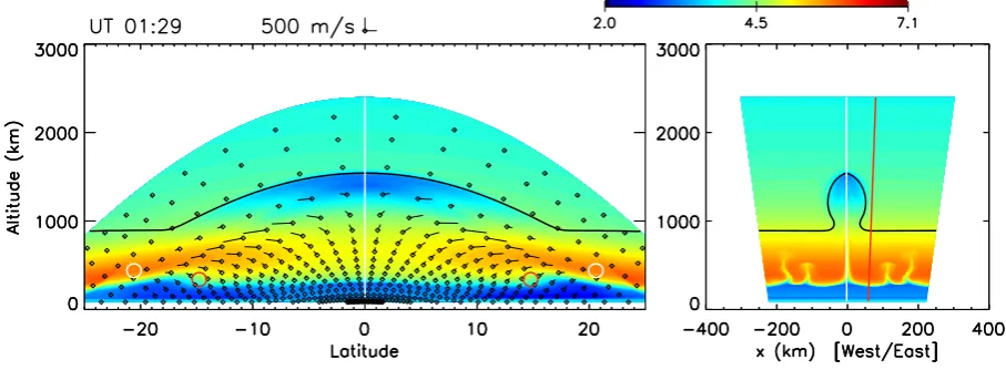
Fig. 1. Contours of log10ne at a fixed longitude (left) and at the magnetic equator (right). The location of the left-hand contour in the
right-hand panel is indicated by a white line and vice versa. Ionization crests are indicated within the ESF plume (white circles) and in the background (red circles). A dark curve near the center of each plot indicates the H+/O+transition height. In the left hand panel, O+ion velocity vectors indicate the direction of flow away from the dot.
and longitude in the magnetic equatorial plane. The grid is periodic in longitude. In essence we are simulating a narrow “wedge” of the ionosphere in the post-sunset period. Unless noted, the ESF instability in each simulation was initiated by imposing a Gaussian-like perturbation in the ion density att=0: a peak ion density perturbation of 15% centered at 0◦ longitude with a half-width of 0.25◦, and at an altitude z=300 km with a half-width of 50 km. This seed perturbation extends along the entire flux tube. For this study, the vertical and zonal neutral winds are set to zero and the meridional neutral wind is set either to zero or to a constant value of 10 m/s.
3 ESF density enhancements
While ESF density depletions are common, both in the sim-ulations and in a wealth of observations, density enhance-ments associated with ESF are seen less often (Watanabe and Oya, 1986; Le et al., 2003; Park et al., 2008b). We first de-scribe the forces that support ionization crests within an ESF plume. We will then consider two situations in which the rel-atively high densities at or above these ionization crests can become ESF density enhancements.
3.1 Ionization crests with an ESF plume
Figure 1 shows an example of a simple ESF plume viewed in the plane of the magnetic equator (right panel) and in a constant longitude plane (left panel). In this case there are no winds (Vns=0). Contour plots show values of log10(ne),
with the location of the left (right) contour plot being indi-cated by a white line in the right-hand (left-hand) panel. The edge of the ESF plume, which has an apex height of 1610 km,
can be seen in both panels as a discontinuity in the density. The left-hand panel shows the flow of O+ions, where veloc-ity vectors indicate the direction of flow away from the dot in each case. A dark curve near the center of each plot indicates the H+/O+transition height, where the densities of these two ionospheric constituents are equal. That the bulk of the ESF plume lies below this transition height at all times is indica-tive of the transport of low-altitude-composition plasma to high altitude, as found by Huba et al. (2009b).
As was seen in past studies (Huba et al., 2008, 2009a,b; Krall et al., 2009a,b), the ESF plume is strongly depleted near its apex, E×B drifts move ions upward across field lines, gravity moves ions downwards along field lines (Han-son and Bamgboye, 1984), and a pair of ionization crests form within the ESF plume, here at altitude 440 km and lati-tude±21◦. These are marked in the left-hand panel by white circles.
For comparison to the ionization crests within the ESF plume, we considered the properties of the background IA at a position indicated by the red vertical line in the right-hand panel of Fig. 1. This is outside of the region affected by the localized electric potential of the nearby ESF plume. The position of the two background IA crests are indicated by red circles in the left-hand panel. We see that the ESF crests occur at an altitude above that of the background IA crests. Further, the ESF crests lie on a field line with an apex altitude above that of the background IA. In Fig. 1 (left panel) field lines are indicated by the black dots at the base of each vector; these dots are arrayed along selected field lines.
Past studies of the “fountain effect” that leads to the IA (Hanson and Moffett, 1966; Anderson, 1973) show that the crest positions are dependent on the magnitude of the upward
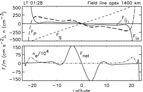
Fig. 2. Field-aligned gravity (Fg, dashed line) and diffusion (Fin,
solid) forces acting on O+ions are indicated within the ESF plume (top panel) and in the background ionosphere (bottom panel) for field lines corresponding to the ionization crests in each case. Elec-tron density (dot-dash) is also plotted.
on geomagnetic field lines of higher altitude. These stud-ies have also shown that the position of the IA crests along the geomagnetic field is governed by a balance between the downward gravitational force and the upward diffusion force that is exerted by neutrals on the downward-moving ions (see Eq. 6). This is illustrated in Fig. 2, where the electron density (dot-dash line) is plotted along with two of the forces act-ing on O+ions: the acceleration due to gravityFg/mi=gs
(dashed) and the acceleration due to ion-neutral diffusion, Fin/mi= −νinVis (solid). These forces are plotted versus
latitude for the field line and longitude corresponding to the ESF crests (top panel) and for the background IA crests (bot-tom panel). In both cases, we see that the peak in the den-sity occurs where the gravitational and diffusive forces are approximately equal in magnitude. To our knowledge, this is the first demonstration that the IA crests do indeed peak where the gravitational and diffusive forces are equal and op-posite.
A more detailed look at the forces acting on O+ ions within the ESF plume is shown in Fig. 3, where each of the five terms on the right-hand side of Eq. (6) is plotted in the upper panel. As in Fig. 2 (top), the plot is along the field line corresponding to the ionization crests within the ESF plume shown in Fig. 1. The lower panel of Fig. 3 shows the net force and the electron density. That the ionization crests within the ESF plume are held in place primarily by the downward grav-ity (Fg) and upward diffusion (Fin) forces is confirmed in
Fig. 3 (top), which shows that the ion and electron pressures are approximately zero where the electron density peaks and that the ion-ion diffusion forceFijis everywhere small.
[image:4.595.55.281.62.215.2]Fig-ure 3 (bottom) shows that the ionization crests are in a near-equilibrium state, with the net force being close to zero in the crest regions.
Fig. 3. Top panel: field-aligned forces, gravity (dashed line), ion and electron pressures (long-dashed lines), and diffusion (Fin,Fij,
solid lines), acting on O+ions are indicated for a field line corre-sponding to the ionization crests within the plume. Bottom panel: net field-aligned force (solid line) acting on O+ ions is plotted. Electron density (dot-dash) is also shown.
These results further demonstrate the workings of the ESF “super fountain,” which was first identified by Huba et al. (2009b). Through this and other three-dimensional ESF sim-ulations, we find that the largeE×B drifts within the ESF plume create ionization crests on field lines above those of the background IA crests. We also find that the large pole-ward field-aligned ion velocities within the plume result in large ion-neutral diffusive forces that support these ioniza-tion crests at altitudes above those of the background IA crests. The diffusive force is interesting in that it is only sig-nificant when ion (or neutral) velocities are large. However, we shall see in the next section that even a weakly growing ESF plume can generate velocities of 100–200 m/s and that these are large enough to support ionization crests at alti-tudes higher than those of the background IA crests. Further results (not shown) show thatFinis dominated by collisions
between O+and O; when the contribution from this interac-tion is removed, the crests appear at a much lower altitude. The importance of O+/O collisions raises the possibility that the “Burnside factor” (Jee et al., 2005), which may increase the O+/O collisions rate by a factor as large as 1.8, may have some effect. However, becauseFin varies so rapidly at the
crest altitude (see Fig. 2), we find that this factor is of little importance to the position of the crests. Similarly, we con-sidered the effect of of ion heating within the plume, which was found by Huba et al. (2009a). This was also found to be of little consequence. Indeed, the most significant fac-tor in determining the height of the crests appears to be the downward, field-aligned ion velocity: larger velocities lead to higher crest altitudes.
While our analysis shows that the ion-ion diffusive force Fij is of little consequence to the positions of ionization
J. Krall et al.: ESF density enhancements 331
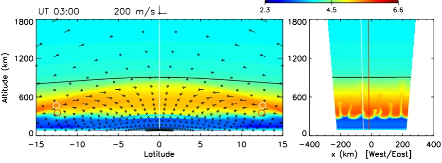
Fig. 4. Contours of log10ne at a fixed longitude (left) and at the magnetic equator (right). The location of the left-hand contour in the
right-hand panel is indicated by a white line and vice versa. Ionization crests are indicated within the ESF plume (white circles) and in the background (red circles). A dark curve near the center of each plot indicates the H+/O+transition height. In the left hand panel, O+ion velocity vectors indicate the direction of flow away from the dot.
observable in situ. As implied by Huba et al. (2009b),Fij
within the upper part of plume is dominated by the interplay between O+and H+ions, with the downward flow of the O+ “super fountain” initially dragging H+downward and out of hydrostatic equilibrium, followed by oscillations in the H+ velocity and, consequently,Fij. Figure 3 (top) showsFij,
the force exerted by H+on O+, during a phase in which H+ is moving upwards. Oscillations in the H+ density also af-fect the ion and electron pressure terms near the apex of the plume.
3.2 Density enhancements associated with weakly grow-ing ESF
We now consider a case in which ESF develops with a low growth rate and without the occurrence of a strong super fountain (Huba et al., 2009b) within the ESF plume. Specif-ically, we consider a simulation where ESF plumes grow from random fluctuations in the ion density, temperature, and velocity instead of from a “seed” perturbation as in Fig. 1. The fluctuations were applied to the initial condi-tions only and were given characteristic amplitudes that var-ied versus height in such a way that fluctuation amplitudes everywhere correspond to the observed amplitudes of trav-eling ionospheric disturbances (TIDs) as reported in Hocke and Schlegel (1996, see Fig. 17 therein). For simplicity, the fluctuations were applied only to O+. Initial fluctuations are consistent with the TID observations only in terms of fluctu-ation amplitude versus height; we did not otherwise mimic TIDs. Outside of the height range of the reported observa-tions, fluctuation amplitude versus height falls smoothly to zero such that there are no fluctuations below 50 km or above 900 km. This simulation, shown in Fig. 4, is otherwise iden-tical to that shown in Fig. 1.
Figure 4 (right) shows that several ESF plumes grow within the simulation. Figure 4 (left) shows density (log10ne)
contours and velocity vectors within one of the ESF plumes. As in Fig. 1, the location of the left (right) contour plot is in-dicated by a white line in the right-hand (left-hand) panel. As in Fig. 1, ionization crests within the ESF plume are marked by white circles and the position of the background IA crests are marked by red circles. We see that, once again, the ESF ionization crests occur on a field line above that of the back-ground IA crests and at an altitude above the backback-ground IA. The left-hand panel also shows the flow of O+ions, where velocity vectors indicate the direction of flow away from the dot in each case.
This simulation includes several interesting features. Be-cause ESF is not a simple local instability (Rishbeth, 1971; Zalesak et al., 1982), ESF growth is dependent on the specifics of the three-dimensional initial perturbation. That ESF growth rates depend on field-line integrated quantities such as the Pedersen conductivity was verified by Krall et al. (2009a), who computed these growth rates for comparison to SAMI3/ESF simulation results. In fact, properties of the optimum naturally-occurring ESF seed have not yet been de-termined. For this TID-like initial perturbation, we find that ESF plumes grow more slowly than the “seeded” plume of Fig. 1 above, which reached a very high altitude as a result of the artificially-large initial density perturbation (15%). At 03:00 local time the plume of Fig. 4 (left) has only reached an apex height of 850 km. We emphasize that the initial seed perturbation is the only difference between these two cases.
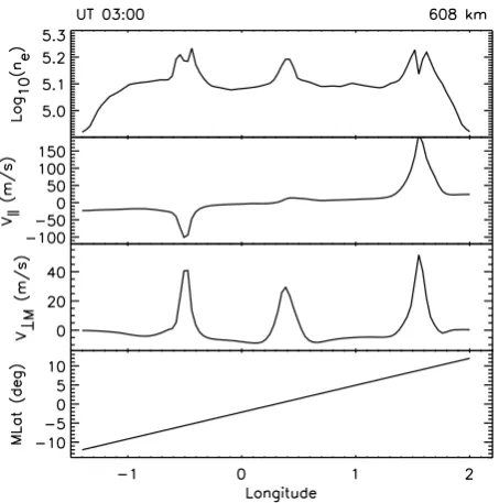
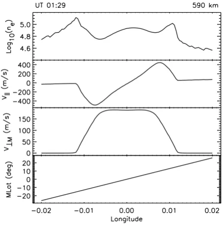
Fig. 5. Plots of log10ne, field-aligned O+velocity (Vk, positive =
northward), verticalE×Bvelocity (V⊥M), and magnetic latitude
versus longitude along a trajectory fixed altitude 608 km.
the edge of the ESF plume is indicated by a discontinuity in log10(ne). Figure 4 (right) shows that the density is enhanced
relative to the background only near the top of each plume (at altitudes of 600 to 850 km for the plume cross-section shown in the left-hand panel).
In fact, the simulation shows multiple plumes, all with density enhancements at these heights. The three tallest ESF plumes, all with apex heights above 600 km, can be seen in Fig. 4 (right), and in Fig. 5. This figure shows plots of log10ne, field-aligned O+velocity, vertical E×Bvelocity,
and magnetic latitude versus longitude along a trajectory at fixed altitude 608 km. The top panel shows density increases similar to those seen in satellite data (Oya et al., 1986; Le et al., 2003; Yokoyama et al., 2007; Park et al., 2008b; Marti-nis et al., 2009). We see that theE×Bdrifts are everywhere upward and that the field aligned flows are everywhere pole-ward. These are also characteristic of the satellite data (com-parisons to the data will be discussed further below).
As in the case shown in Fig. 1, the density crests are held up by the ion-neutral diffusive force acting against the gravity-driven downward ion flow. The key to this result ap-pears to lie in the relative weakness in the ESF super foun-tain in this case (note the change in the scale for the velocity vectors in Fig. 4 versus Fig. 1). The relatively weak seed, combined with effect of the low F10.7 index (F10.7=75 in all runs), leads to a plume in which a strong depletion at high altitude is never obtained. The field-aligned velocities are nevertheless strong enough that the upward diffusion force is able to support both the ESF ionization crests and the
en-hanced densities that extend upwards along the ionization-crest field lines to their apex. In our simulations to date, this situation has only occurred for low values (<100) of the F10.7 index.
3.3 Density enhancements associated with meridional winds
We now consider the situation in which a meridional wind alters the plume and background densities in such a way that one of the ionization crests shown in Fig. 1 above be-comes a density enhancement. Figure 6 shows a simulation with parameters identical to that of Fig. 1, but with a con-stant meridional wind of 10 m/s. Similar to the model results shown in Krall et al. (2009b, see Figs. 4 and 5 therein) this wind is strong enough to introduce a north-south asymme-try into the background ionospheric density while being too weak to suppress the growth of ESF (Krall et al., 2009a). In the case of Fig. 6, however, the EUV indices and the wind speed are much lower than in Krall et al. (2009b), where F10.7=F10.7a=170 andVn=20 m/s were used.
Figure 6 shows the ESF plume in a constant-longitude plane (left panel). As expected from past theoretical (Maruyama, 1988; Zalesak and Huba, 1991; Sultan, 1996) and numerical efforts (Sultan, 1996; Krall et al., 2009a), the wind reduces the growth of the ESF plume relative to the case with no wind (Fig. 1). Here contour plots show values of log10(ne), with the location of the left (right) contour plot
being indicated by a white line in the right-hand (left-hand) panel. The left-hand panel also shows the flow of O+ ions, where velocity vectors indicate the direction of flow away from the dot in each case. As in Figs. 1 and 4 above, ioniza-tion crests within the ESF plume (white circles) occur at an altitude and on a field line above those of the background IA crests (red circles). Plots (not shown) of forces acting along a field line corresponding to the ionization crests within the plume verify that, once again, ionization crests are located where the gravitational and diffusion forces are in balance.
The edge of the ESF plume, which has an apex height of 1090 km, can be seen in the left-hand panel as a discon-tinuity in the density. As in Fig. 4, the density inside the plume is not always lower then the adjacent density outside the plume. In the northern “leg” of the plume, 12◦N, 700 km, the density is noticeably higher than the nearby density out-side of the plume. The density enhancement can also be seen in the right-hand panel, which here shows contours of log10(ne)versus longitude and altitude along a surface that
slices through the northern half of simulation; this surface is indicated by the white curve in the left-hand panel. At lon-gitude 0 and at heights of 580–720 km, the right-hand panel shows electron densities higher than those of the background at the same altitude. By contrast, the density in the southern leg of the plume is lower than that of the background.
J. Krall et al.: ESF density enhancements 333
Fig. 6. Contours of log10neat a fixed longitude (left) and in a surface that slices through the northern “leg” of the ESF plume (right). The
location of the left-hand contour in the right-hand panel is indicated by a white line and vice versa. Ionization crests are indicated within the ESF plume (white circles) and in the background (red circles). A dark curve near the center of each plot indicates the H+/O+transition height. In the left hand panel, O+ion velocity vectors indicate the direction of flow away from the dot.
densities are evident in Fig. 7, which shows plots of log10ne,
field-aligned O+velocity, verticalE×Bvelocity, and mag-netic latitude versus longitude along a trajectory at fixed al-titude 590 km. Note that while the format of this figure is similar to that of Fig. 5 above, the trajectory in this case is along a nearly-constant longitude such that it slices through both the northern and southern legs of the ESF plume shown in Fig. 6. In the top panel of Fig. 7 we see that the back-ground electron density is about 105cm−3at latitude−15◦, that the density drops at the southern edge of the plume (the interior of the plume is indicated by large field-aligned and upward velocities), that the density climbs to about 105cm−3 inside the northern leg of the plume (latitude 15◦), and that the background density just outside of the northern leg of the plume drops to about 5×104cm−3. Of the two peaks in the density curve, only the northern peak is a plasma blob; the southern peak is outside of the plume.
An interesting feature of Figs. 6 and 7 is that north-south density asymmetry within the plume is opposite that of the north-south density asymmetry in the background iono-sphere. As has been seen in past simulations and modeling, a northern wind tends to lift the southern IA crest, reducing its rate of recombination relative to that of the northern crest (e.g., see Fig. 5b of Sultan, 1996, or Fig. 2 of Krall et al., 2009a) . As a result, the southern IA crest obtains a higher density. By contrast, within the ESF plume, the meridional wind appears to shift density from south to north, where it “piles up” at or above the northern ionization crest within the ESF plume. Our interpretation is that the ion density builds up in this region because it is at such a high altitude that sig-nificant recombination does not occur. The result, seen here and in Krall et al. (2009b, see Figs. 4 and 5 therein), is a den-sity enhancement within the northern leg of the ESF plume.
Fig. 7. Plots of log10ne, field-aligned O+velocity (Vk, positive =
northward), verticalE×Bvelocity (V⊥M), and magnetic latitude
versus longitude along a trajectory fixed altitude 590 km.
As in Figs. 4 and 5 above, density enhancements are asso-ciated with upwardE×Bdrifts and poleward field-aligned flows.
3.4 Comparison to data
[image:7.595.314.542.320.550.2]Fig. 8. Data from ROCSAT-1 at altitude 600 km on 21 September 1999: field-aligned ion velocityVk, vertical (meridional) perpendicular ion velocityV⊥M, zonal perpendicular ion velocityV⊥Z, electron densityN, magnetic latitude, and local time plotted versus universal time
and longitude. From Le et al. (2003).
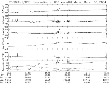
the ROCSAT-1 satellite orbiting at an altitude of about 600 km. Similar results have been obtained using the CHAMP (350 km), Hinotori (650 km), STSAT (680 km), and DMSP (F12, F14, and F15, 800–840 km) satellites, though neither Hinotori nor CHAMP include velocity data (Oya et al., 1986; Le et al., 2003; Park et al., 2008b).
In examining these data, we see features that are simi-lar to those found in the simulation results of Figs. 5 and 7 above. In all cases, density enhancements represent in-creases of about 50–100% over background densities and ion velocities within the enhancements are upward and pole-ward. For example, similar to Fig. 8, Fig. 5 shows that the parallel ion velocity within the enhancements changes sign as the trajectory line crosses the magnetic equator. We also
J. Krall et al.: ESF density enhancements 335
Fig. 9. Data from ROCSAT-1 at altitude 600 km on 8 March 2004: vertical (meridional) perpendicular ion velocityV⊥M, zonal perpendicular ion velocityV⊥Z, field-aligned ion velocityVk, electron density logN, and O+, H+, and He+composition plotted versus universal time, longitude and dip latitude. From Yokoyama et al. (2007).
distances further from the magnetic equator (however, Fig. 8 does not). A more extensive study of density-enhancement data could determine whether or not this is a common pat-tern.
4 Conclusions
Using the NRL SAMI3/ESF three-dimensional simulation code, we have examined the forces governing the formation of the density crests that occur within an ESF plume as a re-sult of the ESF “super fountain effect” (Huba et al., 2009b). As with the IA crests that usually occur in the post-sunset equatorial ionosphere, we find that ESF density crests are located where downward gravity and upward ion-neutral dif-fusive forces are in balance. We have shown that largeE×B
drifts within the ESF plume place these crests on field lines above those of the background IA crests in all cases. Sim-ilarly, large poleward field-aligned ion velocities within the plume result in large ion-neutral diffusive forces that support
these ionization crests at altitudes higher than those of the background IA crests in all cases.
We have shown two circumstances in which the density on or above the ESF crests leads to a density enhancement, also called a “plasma blob,” similar to those observed in situ (Oya et al., 1986; Watanabe and Oya, 1986; Le et al., 2003; Yokoyama et al., 2007; Park et al., 2008b; Martinis et al., 2009). In one case, slowly growing ESF produces upward
E×B drifts that move density upward faster than gravity moves it downward, with the result that densities on ESF-crest field lines, at or above the density ESF-crests, have densi-ties that are enhanced relative that of the background iono-sphere. In this case the ESF super fountain is relatively weak, with velocities of order 200 m/s. In our simulations to date, this situation has only occurred for low values (<100) of the F10.7 index.
relatively high altitude, a meridional wind has an effect on the ESF crests that differs from its effect on the IA crests. Whereas a northward wind raises the southern IA crest, re-ducing recombination, and lowers the northern crest, en-hancing recombination, a meridional wind acting on an ESF plume simply pushes plasma northward, causing a slight in-crease in the density of the northern crest (because the ESF crests occur at relatively high altitude, they are not strongly affected by recombination). As a result, in the presence of a mild northward meridional wind (10 m/s in this case), the northern ESF crest can become a density enhancement. Be-cause we have simulated this phenomenon for a variety of circumstances (e.g. Fig. 5 of Krall et al., 2009b), we specu-late that this may be a relatively common occurrence. Watan-abe and Oya (1986) report that plasma blobs occur most of-ten at a distance of 20–30◦away from the magnetic equator, which is consistent with our results with a non-zero merid-ional wind. In addition, both Watanabe and Oya (1986) and Park et al. (2008b) report a higher occurrence of blobs in the winter hemisphere, a circumstance which favors a trans-equatorial meridional wind.
Finally we have shown that the simulated density enhance-ments have properties similar to that of observed density en-hancements, also called “plasma blobs” (Oya et al., 1986; Le et al., 2003; Yokoyama et al., 2007; Park et al., 2008b; Martinis et al., 2009). In all cases, density enhancements represent increases of 50–100% over background densities as observed. Further, ion velocities within the enhancements are upward and poleward in all cases, as is typically observed (Le et al., 2003; Yokoyama et al., 2007; Martinis et al., 2009). We note that observed blobs show a compositional signa-ture (increased O+/H+ ratio, Yokoyama et al., 2007) that is characteristic of lower-altitude ionospheric plasma that has been lifted upwards, as in our simulations (Huba et al., 2009b). As is seen in the observations, our simulations show that ESF-like depletions and enhancements occur simultane-ously in the same region of the upper ionosphere (Oya et al., 1986; Watanabe and Oya, 1986; Le et al., 2003; Park et al., 2008b; Martinis et al., 2009). This association of density enhancements and ESF activity has been further verified by Yokoyama et al. (2007), who report simultaneous ROCSAT-1 and radar observations showing that an enhancement in one hemisphere can co-exist with a depletion in the other hemi-sphere on the same flux tube (see also Fig. 7 above), and Mar-tinis et al. (2009), who show that density enhancements are co-located on the same field lines as ESF airglow enhance-ments (see also Krall et al., 2009b).
We conclude, consistent with Le et al. (2003) and Martinis et al. (2009), that these density enhancements are signatures of ESF. However, we find that the enhanced densities are sup-ported by the enhanced ion-neutral diffusive forces that are associated with the high field-aligned ion velocities of the ESF super fountain rather than a wind-driven instability in the topside ionosphere, as suggested by Watanabe and Oya (1986), or pressure forces, as suggested by Le et al. (2003).
We further assert that, while ESF plume densities are gener-ally much lower than surrounding ionospheric densities, typ-ical ESF plumes nevertheless contain regions in which the plume density is close to or greater than that of the back-ground ionosphere.
Acknowledgements. The authors would like to thank Sidney Os-sakow of Berkeley Research Associates for helpful discussions. This work was supported by the Office of Naval Research and NASA.
Topical Editor K. Kauristie thanks two anonymous referees for their help in evaluating this paper.
References
Anderson, D. N.: A theoretical study of the ionosphericF region equatorial anomaly–I. Theory, Planet. Space Sci., 21, 409–419, 1973.
Booker, H. G. and Wells, H. W.: Scattering of radio waves in the F-region of ionosphere, Terr. Mag. Atmos. Elec., 43, 249–256, 1938.
de La Beaujardiere, O., Jeong, L., and The C/NOFS Science Def-inition Team: C/NOFS: a mission to forecast scintillations, J. Atmos. Solar Terr. Phys., 66, 1573–1591, 2004.
Haerendel, G.: Theory of equatorial spreadF, preprint, Max Planck Inst. Extraterr. Phys., Munich, Germany, 1974.
Hanson, W. B. and Bamgboye, D. K.: The measured motions inside equatorial plasma bubbles, J. Geophys. Res., 89, 8997–9008, 1984.
Hanson, W. B. and Moffett, R. J.: Ionization transport effects in the equatorialF region, J. Geophys. Res., 71, 5559–5572, 1966. Hocke, K. and Schlegel, K.: A review of atmospheric gravity waves
and travelling ionospheric disturbances: 1982–1995, Ann. Geo-phys., 14, 917–940, 1996,
http://www.ann-geophys.net/14/917/1996/.
Huba, J. D., Joyce, G., and Fedder, J. A.: SAMI2 (Sami2 is An-other Model of the Ionosphere): A New Low-Latitude Iono-sphere Model, J. Geophys. Res., 105, 23035–23053, 2000. Huba, J. D., Joyce, G., Sazykin, S., Wolf, R., and Shapiro, R.:
Simulation study of penetration electric fields in the low- to mid-latitude ionosphere, Geophys. Res. Lett., 32, L23101, doi: 10.1029/2005GL024162, 2005.
Huba, J. D., Joyce, G., and Krall, J.: Three-dimensional equatorial spreadF modeling, Geophys. Res. Lett., 35, L10102, doi:10. 1029/2008GL033509, 2008.
Huba, J. D., Joyce, G., Krall, J., and Fedder, J.: Ion and electron temperature evolution during equatorial spread-F, Geophys. Res. Lett., 36, L15102, doi:10.1029/2009GL038872, 2009a. Huba, J. D., Krall, J., and Joyce, G.: Atomic and molecular ion
dynamics during equatorial spread-F, Geophys. Res. Lett., 36, L10106, doi:10.1029/2009GL037675, 2009b.
Hysell, D. L.: An overview and synthesis of plasma irregularities in equatorial spreadF, J. Atmos. Solar Terr. Phys., 62, 1037–1056, 2000.
Jee, G., Schunk, R. W., and Scherliess, L.: On the sensitivity of the total electron content (TEC) to upper atmospheric/ionospheric parameters, J. Atmos. Solar Terr. Phys., 67, 1040–1052, 2005. Kelley, M. C.: The Earth’s Ionosphere, Plasma Physics and
J. Krall et al.: ESF density enhancements 337 Krall, J., Huba, J. D., Joyce, G., and Zalesak, S. T.:
Three-dimensional simulation of equatorial spread-F with meridional wind effects, Ann. Geophys., 27, 1821–1830, 2009a,
http://www.ann-geophys.net/27/1821/2009/.
Krall, J., Huba, J. D., and Martinis, C.: Three dinensional model-ing of equatorial spread-Fairglow enhancements, Geophys. Res. Lett., 36, L10103, doi:10.1029/2009GL038441, 2009b. Le, G., Huang, C.-S., Pfaff, R. F., Su, S.-Y., Yeh, H.-C., Heelis,
R. A., Rich, F. J., and Hairston, M.: Plasma density en-hancements associated with equatorial spread F: ROCSAT-1 and DMSP observations, J. Geophys. Res., ROCSAT-108, ROCSAT-13ROCSAT-18, doi:10.1029/2002JA009592, 2003.
Martinis, C., Baumgardner, J., Mendillo, M., Su, S.-Y., and Aponte, N.: Brightening of 630.0 nm airglow depletions ob-served at midlatitudes, J. Geophys. Res., 114, A06318, doi: 10.1029/2008JA013931, 2009.
Maruyama, T.: A diagnostic model for equatorial spread-F 1. Model description and application to electric field and neutral wind effects, J. Geophys. Res., 93, 14611–14622, 1988. Maruyama, T., Saito, S., Kawamura, M., Nozaki, K., Krall, J.,
and Huba, J. D.: Equinoctial asymmetry of a low-latitude ionosphere-thermosphere system and equatorial irregularities: evidence for meridional wind control, Ann. Geophys., 27, 2027– 2034, 2009,
http://www.ann-geophys.net/27/2027/2009/.
Ossakow, S. L.: SpreadF theories: A review, J. Atmos. Terr. Phys., 43, 437–452, 1981.
Oya, H., Takahashi, T., and Watanabe, S.: Observation of low lat-itude ionosphere by the impedance probe on board the Hinotori satellite, J. Geomag. Geoelectr., 38, 111–123, 1986.
Oyama, K.-I., Schlegel, K., and Watanabe, S.: Temperature struc-ture of plasma bubbles in the low latitude ionosphere around 600 km altitude, Planet. Space Sci., 36, 553–567, 1988. Park, J., Min, K. W., Kim, V. P., Kil, H., Su, S.-Y., Chao, C. K.,
and Lee, J.-J.: Equatorial plasma bubbles with enhanced ion and electron temperatures, J. Geophys. Res., 113, A09318, doi:10. 1029/2008JA013067, 2008a.
Park, J., Stolle, C., L¨uhr, H., Rother, M., Su, S.-Y., Min, K. W., and Lee, J.-J.: Magnetic signatures and conjugate features of low-latitude plasma blobs as observed by the CHAMP satellite, J. Geophys. Res., 113, A09313, doi:10.1029/2008JA013211, 2008b.
Picone, J. M., Hedin, A. E., Drob, D. P., and Aikin, A. C.: NRLMSISE-00 empirical model of the atmosphere: Statistical comparisons and scientific issues, J. Geophys. Res., 107, 1468, doi:10.1029/2002JA009430, 2002.
Retterer, J. M.: Forecasting low-latitude radio scintillation with 3-D ionospheric plume models: 1. Plume model, J. Geophys. Res., doi:10.1029/2008JA013839, in press, 2009a.
Rishbeth, H.: Polarization fields produced by winds in the equato-rialF region, Planet. Space Sci., 19, 357–369, 1971.
Scherliess, L. and Fejer, B. G.: Radar and satellite global equatorial Fregion vertical drift model, J. Geophys. Res., 104, 6829–6842, 1999.
Steenburgh, R. A., Smithtro, C. G., and Groves, K. M.: Ionospheric scintillation effects on single frequency GPS, Space Weather, 6, S04D02, doi:10.1029/2007SW000340, 2008.
Sultan, P. J.: Linear theory and modeling of the Rayleigh-Taylor instability leading to the occurrence of equatorial spreadF, J. Geophys. Res., 101, 26875–26891, 1996.
Watanabe, S. and Oya, H.: Occurence characteristics of low latitude ionosphere irregularities observed by impedance probe on board the Hinotori satellite, J. Geomag. Geoelectr., 38, 125–149, 1986. Yokoyama, T., Su, S.-Y., and Fukao, S.: Plasma blobs and ir-regularities concurrently observed by ROCSAT-1 and Equato-rial Atmosphere Radar, J. Geophys. Res., 112, A05311, doi: doi:10.1029/2006JA012044, 2007.
Zalesak, S. T. and Huba, J. D.: Effect of meridional winds on the development of equatorial spread-F, Eos Trans. AGU, 72, Spring Meet. Suppl., 211, 1991.