www.ann-geophys.net/28/1333/2010/ doi:10.5194/angeo-28-1333-2010
© Author(s) 2010. CC Attribution 3.0 License.
Annales
Geophysicae
Quantitative relation between PMSE and ice mass density
S. Kirkwood1, M. Hervig2, E. Belova1, and A. Osepian3 1Swedish Institute of Space Physics, Kiruna, Sweden 2GATS Inc., Driggs, ID 83422, USA
3Polar Geophysical Institute, Murmansk, Russia
Received: 25 March 2010 – Revised: 17 June 2010 – Accepted: 18 June 2010 – Published: 23 June 2010
Abstract. Radar reflectivities associated with Polar
Meso-sphere Summer Echoes (PMSE) are compared with measure-ments of ice mass density in the mesopause region. The 54.5 MHz radar Moveable Atmospheric Radar for Antarc-tica (MARA), located at the Wasa/Aboa station in AntarcAntarc-tica (73◦S, 13◦W) provided PMSE measurements in December 2007 and January 2008. Ice mass density was measured by the Solar Occultation for Ice Experiment (SOFIE). The radar operated continuously during this period but only measure-ments close to local midnight are used for comparison, to coincide with the local time of the measurements of ice mass density. The radar location is at high geographic latitude but low geomagnetic latitude (61◦) and the measurements were made during a period of very low solar activity. As a result, background electron densities can be modelled based on so-lar illumination alone. We find a close correlation between the time and height variations of radar reflectivity and ice mass density, at all PMSE heights, from 80 km up to 95 km. A quantitative expression relating radar reflectivities to ice mass density is found, including an empirical dependence on background electron density. Using this relation, we can use PMSE reflectivities as a proxy for ice mass density, and es-timate the daily variation of ice mass density from the daily variation of PMSE reflectivities. According to this proxy, ice mass density is maximum around 05:00–07:00 LT, with lower values around local noon, in the afternoon and in the evening. This is consistent with the small number of previ-ously published measurements and model predictions of the daily variation of noctilucent (mesospheric) clouds and in contrast to the daily variation of PMSE, which has a broad daytime maximum, extending from 05:00 LT to 15:00 LT, and an evening-midnight minimum.
Keywords. Atmospheric composition and structure (Middle
atmosphere – composition and chemistry)
Correspondence to: S. Kirkwood ([email protected])
1 Introduction
It has been known for many decades that clouds form at very high altitudes (80–90 km), in high latitude regions, in sum-mer. These are visible from the ground as noctilucent clouds (NLC). Their formation is explained by the extremely low temperatures at these summer mesopause heights which are a result of the mesospheric circulation, with upwelling over the summer polar region. Since the 1980s it has also been clear that extremely strong radar echoes can be obtained from the same height region. These are known as Polar Mesosphere Summer Echoes (PMSE). Intensive research using radars, li-dars, satellite remote sensing instruments and in-situ probes carried on sounding rockets has firmly established a relation-ship between extremely cold temperatures, PMSE and noc-tilucent clouds. However, the rather large ice-particles which constitute detectable noctilucent clouds, are found only in the lower part of the PMSE layer. It has been presumed that the upper parts of the PMSE layer are associated with ice par-ticles which are too small to be detected, or with meteoric smoke. In order for smoke or ice particles to generate strong radar scatter, the particles must be electrically charged so that they can cause persistent irregularities in the background gas of free electrons. A small number of sounding rocket exper-iments have tried to measure these particles, and some cor-relations between particles and PMSE have been found, but the nature of the particles causing PMSE, meteoric smoke or ice, has not yet been firmly established (for a recent review see e.g. Rapp and L¨ubken, 2004).
hours around noon (Fiedler et al., 2005). The one satellite instrument which has been able to estimate the local time variation of polar mesospheric clouds (PMC) has also found a minimum between 09:00 and 16:00 LT, with peaks around 06:00 and 18:00 LT (at about 55◦N) (Stevens et al., 2009). This is likely due to tidal variations in temperature and trans-port. PMSE have a distinctly different daily variation from noctilucent clouds, being strongest around noon and weakest in the evening, in both hemispheres (e.g. Nilsson et al., 2008; Smirnova et al., 2010). If PMSE are caused by the same (or similar, but smaller) ice particles as noctilucent clouds we might expect a better correlation. Since PMSE are thought to require ionisation as well as particles, it is possible that the daily variation of ionisation sources is important. Since most studies up to now have been made in the Northern-Hemisphere auroral zone, this aspect has been difficult to quantify. While the daily variation due to solar radiation is easy to predict, the contribution from energetic particles in the auroral zone is highly variable and not easy to measure since even very small numbers of energetic particles can give ionisation in excess of that due to solar radiation.
A number of studies using satellite remote sensing to de-tect clouds at mesopause heights have found evidence of a long-term increase in occurrence frequency (see Shettle et al., 2009, and references therein). However, it has been difficult to correct these observations for possible effects due to local-time variations – the local time of the satellite ob-servations has also changed over time. Obob-servations of the daily variation of noctilucent clouds by lidar cannot be di-rectly used in this context since they are available at only one site up to now (ALOMAR) and, in addition, it is possible that the satellite measurements are not sensitive to the same par-ticle size range. The measurements reported by Stevens et al. (2009) are for only a limited latitude zone (close to 55◦N). If some way can be found to account for the influence of ion-isation on PMSE, and if PMSE can be shown to be due to ice particles, it might be possible to correct for ionisation ef-fects in the local-time variation of PMSE and to use PMSE to estimate the diurnal variation of ice particles. To see if this is possible, we compare direct observations of ice par-ticle characteristics (from a satellite) with measurements of PMSE from Antarctica, where the large difference in geo-graphic and geomagnetic latitudes allows PMSE to be moni-tored with minimal disturbance from auroral precipitation.
2 SOFIE – Solar Occultation for Ice Experiment
The Solar Occultation for Ice Experiment (SOFIE) is a multi-band radiometer onboard the Aeronomy of Ice in the Meso-sphere (AIM) satellite. Details of the AIM satellite mission and the SOFIE instrument can be found in Russell et al. (2009) and Gordley et al. (2009), respectively. SOFIE mea-sures extinction profiles near the time of local sunrise or sun-set, to study PMC characteristics during the summer seasons
in both the Northern and Southern Hemispheres. The latitude of the measurements varies between 66◦(midsummer) and 76◦(start and end of the summer season). The field of view for PMC measurements corresponds to 1.5 km vertically at the tangent point. SOFIE can in principle measure ice mass density (Mice), effective radius, axial ratio, and the parame-ters of a Gaussian size distribution (number concentration, mean radius and distribution width) (Hervig et al., 2009). However, due to decreasing signal-to-noise in the short wave-length measurements, SOFIE often does not obtain reliable particle size or Gaussian parameters at the highest altitudes of PMC layers.
For comparison with PMSE, we select SOFIE ice mass density measurements, since these are available over an ex-tended height interval. We select SOFIE profiles which are measured at geographic locations within 15◦longitude of the radar site. There are 55 such profiles available for the time covered by PMSE measurements, 6 December 2007–30 Jan-uary 2008. The nature of the solar occultation measurements means that they are all taken at close to the same local solar time, in this case, between 01:04 and 01:15 LT. In the middle of the season, the measurements are at latitudes below the polar circle (65.5◦S), whereas at the beginning and end of the period of joint measurements they are at higher latitudes (66.5◦and 71.2◦S, respectively).
There is no a-priori justification for choosing ice mass density to compare with PMSE, but as we shall see later, it in practice turns out to provide a good correlation. SOFIE provides unprecedented sensitivity and measures ice mass-density directly, throughout the height interval where PMSE are observed, making this parameter particularly good in this context. It might also be noted that Rapp et al. (2003) have argued that the quantityZNicer2 , whereZ is the average charge per particle,Niceis the number of ice particles, andr is the mean particle radius, can be used as a proxy for PMSE.
Zis expected to increase with increasingr, such thatZ∝r, at least for ice particles with at least 10 nm radius (Jensen and Thomas, 1991). So the proxy becomes∝Nicer3 , i.e. proportional to ice mass density.
3 MARA – Moveable Atmospheric Radar for Antarctica
and the instrument-independent parameter volume reflectiv-ity (η) is calculated from the radar echo power. The radar cy-cles between modes optimised for PMSE, tropospheric and boundary layer studies, providing one profile in each mode every 2 min, each profile representing an average over about 40 s. More details of the MARA radar, operating modes and calibration can be found in Kirkwood et al. (2007).
The longest period of radar operations so far was at the Swedish/Finnish Antarctic station Wasa/Aboa (73◦S, 13◦W) from 4 December 2007 to 31 January 2008. PMSE observations from MARA during this season have already been reported in Kirkwood et al. (2008), where attention was drawn to the unusual behaviour of the PMSE height, starting with the middle of the PMSE layer above 90 km in early De-cember 2007 and descending to the height near 85 km, which is usual in the Northern Hemisphere, only after the solstice. This was found to be related to a similar height shift in the location of the coldest temperatures.
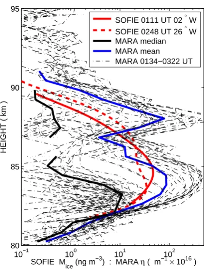
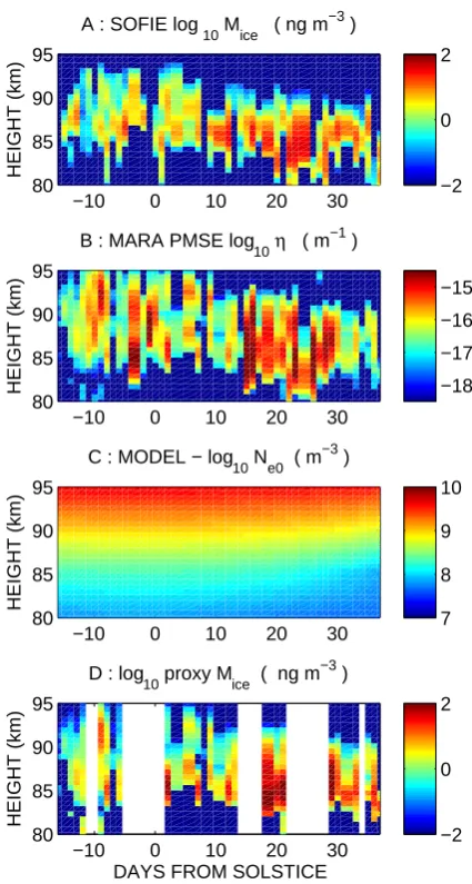
[image:3.595.322.534.58.336.2]4 Comparison of PMSE and ice mass density
Figure 1 shows an example of simultaneous, closely co-located observations from MARA and from SOFIE. SOFIE measured two profiles of ice mass density within 15◦ lon-gitude and 2◦ latitude of MARA, about 2 h apart (on con-secutive orbits). Both profiles (red lines) are very similar. MARA observations of volume reflectivity are shown from 1 h before to 1 h after the local solar time (at MARA) cor-responding to the local time of the SOFIE measurements. The correlative data is selected in terms of local solar time because of the well-known, strong, local-time variations of PMSE and noctilucent clouds. The PMSE reflectivities are scaled by an arbitrary factor so they can be plotted on the same scale as the SOFIE data. The individual 2-min profiles (dashed lines) show large variability, with the whole profile moving between higher and lower levels as time passes. The mean and median reflectivity profiles (thick blue and black lines, respectively) are quite different to each other, and the shape of the ice mass density profiles (red) is somewhere in between. The wave-like perturbations in the radar reflectivity are likely due to the influence of a long-period gravity wave. Radar reflectivity (for radars operating close to 50 MHz) in the upper troposphere and lower stratosphere is well known to be primarily controlled by the large-scale vertical gradi-ent of radio refractive index (e.g. Gage, 1990; Hooper et al., 2004). It is less well known that a similar sensitivity associ-ated with large-scale gravity waves, has been documented and theoretically explained also in the mesosphere, where the electron density, rather than the neutral density, is re-sponsible for the refractive index gradient (Muraoka et al., 1989). Theoretically, the effect could be explained by the influence of gravity waves on the background gradient of electron density, by amounts which depend on the details of the ion-chemistry controlling the electron loss processes.
10−1 100 101 102
80 85 90 95
SOFIE M ice (ng m
−3) : MARA η ( m−1× 10¹⁶ )
HEIGHT ( km )
SOFIE 0111 UT 02 ° W SOFIE 0248 UT 26 ° W MARA median MARA mean
MARA 0134−0322 UT
Fig. 1. Profiles of ice mass density measured by SOFIE and of PMSE volume reflectivity measured by MARA on 15 January 2008.
Some influence on PMSE can also be expected from vari-ations in the ice-particle microphysics associated with tem-perature changes in the wave (e.g. Hoffmann et al., 2008). However, according to the simulations in the latter paper, the temperature effect seems too little to explain the observed amplitude of the wave-related PMSE variations. In any case, since we would like to find the influence of other parame-ters on PMSE, we need to find a way to average out such wave perturbations. It is clear from Fig. 1 that reflectivities vary by several orders of magnitude under the influence of the wave, so that a median will be a more appropriate esti-mate of average conditions than an arithmetic mean. It is also clear that rather long intervals, in excess of 2 h will likely be needed to average out wave effects. Seasonal averages of the daily variation of PMSE reflectivity in Antarctica (e.g. Mor-ris et al., 2006; Nilsson et al., 2008), on the other hand, show a strong, systematic variation over the day. So we need to confine time-averaging to an interval close in local time to the SOFIE observations. This means that some wave effects will still be present in average (median) profiles from indi-vidual nights.
−10 0 10 20 30 80
85 90 95
HEIGHT (km)
A : SOFIE log
10 Mice ( ng m −3
)
−2 0 2
−10 0 10 20 30
80 85 90 95
HEIGHT (km)
B : MARA PMSE log
10η ( m −1
)
−18 −17 −16 −15
−10 0 10 20 30
80 85 90 95
HEIGHT (km)
C : MODEL − log10 Ne0 ( m−3 )
7 8 9 10
−10 0 10 20 30
80 85 90 95
DAYS FROM SOLSTICE
HEIGHT (km)
D : log10 proxy Mice ( ng m−3 )
[image:4.595.59.272.60.458.2]−2 0 2
Fig. 2. Profiles of ice mass density measured by SOFIE
(panel A) and of PMSE volume reflectivity measured by MARA (panel B) for the period 6 December 2007–30 January 2008. Panel (C) shows model values of background electron density and the panel (D) shows a proxy for ice mass density calculated using observed PMSE volume reflectivity and model electron densities (see text for further details).
summer 2007/2008. The ice is clearly less dense, and lo-cated at higher altitudes, before solstice, descending to lower heights and increasing in density after solstice. Panel (b) in Fig. 2 shows median PMSE reflectivities, from 1 h before to 1 h after the local solar time of the SOFIE measurements (01:04–01:15 LT) have been used. Note that all samples, in-cluding those where the PMSE was at the detection threshold of the radar, are included in determining the median values. The height shift in the PMSE in the middle of the season, as previously reported for whole-day averages by Kirkwood et al. (2008) is clearly seen also in these PMSE profiles from the 00:00–02:00 LT sector..
Overall, the height-time morphologies of ice mass density and volume reflectivity, are quite similar. Both extend to their highest altitudes before solstice, and reach their lowest alti-tudes between 20–30 days after solstice. Double layers are seen by both around 9 days after solstice. Both instruments see a longer period of stronger layers 15–30 days after sol-stice. Some differences can be discerned, however. The ice mass densities are relatively low 10–15 days before solstice, while PMSE reflectivities are rather high at that time. PMSE are relatively weak in the final days of the observations, 30– 38 days after solstice, while ice mass densities remain rela-tively high. PMSE generally remain strong to slightly higher altitude than the ice layer.
The basic mechanism causing PMSE is reflection from irregularities in radar refractive index, with the latter at mesospheric heights controlled primarily by electron den-sity. The relationship between PMSE volume reflectivity (η), electron density (Ne) and ice-particle characteristics is not well established. Rapp et al. (2008) have suggested that η∝(Neω2B/g−δNe/δz−Ne/H )2exp(−γ ), whereωB is bouyancy frequency,gthe acceleration due to gravity,H
the scale height of the neutral atmosphere. In the exponen-tial factor,γdepends on the turbulent energy dissipation rate, the radar wavelength and the Schmidt number but Rapp et al. (2008) argue that, for typical PMSE conditions and for radars operating at about 50 MHz, this exponential term is essen-tially unity. So we might expectηto depend on the square of electron density and/or electron density gradient, depending on the relative magnitudes of the three different terms within the parentheses.
However, the expression in Rapp et al. (2008) is derived assuming that refractive index irregularities are caused by active turbulence and uses equations from Hocking (1985) which are in turn based on the assumption that electron mix-ing ratio is a conservative tracer of vertical motion associ-ated with turbulence. This may not necesarily be appropriate in PMSE conditions where ionisation and charge-exchange reactions between electrons, ions and ice-particles may be faster that the turbulent mixing time scales. Alternative anal-yses consider that electron density fluctuations at the scale causing PMSE are controlled by structures at the same scale in the population of charged aerosol (ice or smoke), which may have been in place for some time. In this case, when there is a plentiful supply of free electrons (NeZNice), electron density fluctuations can be simply proportional to
the middle of the layer, at about 87 km height). We expect
Ne(see discussion below and panel (c) of Fig. 2) to be of the same order so we cannot assumeNeZNice.
When the supply of free elctrons is limited (Ne≤ZNice), the relationship between ice-particle characteristics and radar reflectivity becomes complex, and no simple formulation is possible (Havnes, 2004). However, as mentioned in the last lines of Sect. 3, Rapp et al. (2003) have found empirically that η∝ZNicer2 . Given that we can expect Z∝r, this is equivalent toη∝Nicer3 , i.e. volume reflectivity is pro-portional to ice mass density. Since the latter parameter is measured directly by SOFIE, it is reasonable to test its rela-tionship to radar reflectivity in the present study.
The season 2007/2008 was geomagnetically quiet and MARA, despite its high geographic latitude, lies at rather low geomagnetic latitude (61◦). Although this is well equa-torward of the average auroral zone, there is still a possi-bility of energetic particle precipitation in geomagnetically disturbed conditions (Codrescu et al., 1997). Although our observation period was relatively quiet (mostly with mag-netic Ap index 0–12), there were some days of moderate geomagnetic disturbance (Ap index 15–30). As has been ob-served at Northern Hemisphere auroral zone sites (Smirnova et al., 2010; Bremer et al., 2003), we find, in the present ob-servations, a statistical correlation between PMSE strength and the geomagnetic Ap index. In the MARA data, how-ever, a correlation is found only for Ap≥15. We would like to examine the relationship between PMSE, ice mass den-sity and electron denden-sity so we must restrict our compari-son to quiet conditions (Ap<15), so that we can reasonably model the ionisation conditions on the basis of solar short-wave radiation alone. This can be represented by the qui-escent electron density,Ne0(above 80 km in polar summer, the ionisation rate is proportional toNe02). We use the elec-tron density model described in Smirnova et al. (1988) and Osepian et al. (2008). Results for the location and times cor-responding to the PMSE observations are shown in panel (c) of Fig. 2. Note that the shape of the electron density profiles at PMSE heights is close to exponential so that the vertical gradient of electron density is essentially proportional to the electron density.
On the basis of the considerations outlined above, we try to find a relation of the form ηmed=AMicepN
q
e0 or ηmed= AMicep (δNe0/δz)q, whereδ/δzis the vertical gradient,A,p andq are constants to be determined empirically, andηmed indicates median values over a sufficiently long time to aver-age out gravity-wave effects and possible variations in small-scale processes affecting the fine-structure of the ice-particle distribution. To test the ability of these models to describe the relationship between the parameters, we first make av-erages of η to match the height resolution of the SOFIE measurements, using all joint observations when Ap<15, and all heights between 80 km and 95 km. We then com-pute predicted values according to the empirical models
ηmodel=AMicep Neq0andηgradientmodel =AMicep (δNe0/δz)q, iterat-ing through possible values ofpandq, and testing the corre-lation between the measuredηmedandηmodelin various ways. The simplest way is to compute correlation coefficients for the complete set ofηmedandηmodel values (all heights, all dates) and to find which values ofp andq lead to the best correlation. Overall correlation coefficients are at best low, although significant (rcorr'0.25, but with better than 99% confidence). Correlation coefficients are very similar for a wide range ofpandqso it is difficult to estimate the confi-dence limits of the values found for “best-fit”pandq. Tests with different intervals from the season show dependence on bothNe0 andMice at the beginning and end of the season, but only onMicein the middle of the season. Tests choosing random selections of dates show that the result, the “best-fit” pair of values forpandq, is very dependent on the selection. It is also clear when comparing individual pairs of ice/PMSE profiles that the profile shapes may be very similar but they are often shifted in height, leading to a low correlation. This can easily be a result of wave perturbations since the obser-vations are not at exactly the same location. The best solu-tion to this problem is to use averages over longer intervals. Since our measurements do not follow a normal distribution, and height averaging results in strong correlations between adjacent heights, we need to use a non-parametric method (i.e. one which is not dependent on the statistical properties of the distribution) to get an estimate of confidence limits for
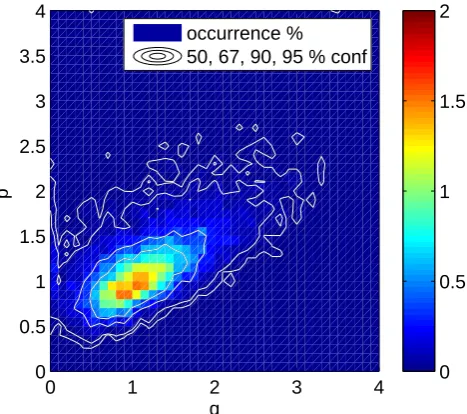
pandq. We use a re-selection method (see e.g. Wilks, 1995), making a large number of random selections of dates to use. For each selection, we average the profiles ofMice,Ne0andη over the dates included, and find the values ofpandqwhich give the best fit to the model. The 2-D histogram of best-fit
pandq pairs forηgradientmodel is shown in Fig. 3 (the histogram forηmodelis essentially the same). Thep,qpair which gives the best fit for the largest number of random trials, can be considered the overall most-likely pair. Various confidence intervals are shown by contours in Fig. 3. The 67% confi-dence contour, for example, encloses the region where 67% of the best-fit pairs lie. We find that the most likely values of
pandqfor both orηgradientmodel andηmodelare close to unity, but values between 0.3 and 2 forq and between 0.5 and 1.5 for
pare within the 67% confidence limits. The results shown in Fig. 3 are for profiles averaged over 25 days, but the re-sults are not significantly different if we select half or twice as many profiles to form the averages. Since we select dates randomly from the whole season in each trial, these values apply to the season as a whole.
0 1 2 3 4 0
0.5 1 1.5 2 2.5 3 3.5 4
q
p
0 0.5 1 1.5 2 occurrence %
[image:6.595.51.285.62.269.2]50, 67, 90, 95 % conf
Fig. 3. Two-dimensional histogram of the occurrence rate
of different values of p and q as best-fit values in ηmed=
AMicep (δNe0/δz)q. Best-fits were obtained using 10 000 random
selections, each of 25 days, averaged to obtainηmedandMice.
Con-fidence intervals are shown by the contours (50% conCon-fidence con-tour innermost). See text for further details.
by our model in the following paragraphs, we consider sim-ply ηgradientmodel and set p=q=1 (which empirically corre-sponds to A=9.0×10⁻²³m6ng−1). (If we were to use
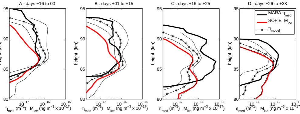
[image:6.595.321.531.65.409.2]ηmodel the appropriate value for p=q=1 would be A= 6.2×10⁻²⁶m5ng−1). Figures 4 and 5 provides illustrations of the agreement between the observations and the empirical model. Panel (a) of Fig. 4 simply illustrates the relationship between volume reflectivity and ice-mass density when indi-vidual days are considered (red crosses) and when averages over several days are used (black symbols). There is clearly a large scatter and the correlation is rather low. Panel (b) of Fig. 4 shows how the correlation is improved by dividing the volume reflectivities by the electron density term (in this case the electron density gradient).
Figure 5 shows measured PMSE and ice mass profiles, av-eraged over four different parts of the season (the same inter-vals as in Fig. 4), compared with the PMSE reflectivity pre-dicted by the model. Here we have plotted the model profiles forp=q=1 and the maximum and minimum values, cor-responding to all sets ofA,p,q within the 67% confidence limits (equivalent to standard deviation). The agreement be-tweenηgradientmodel andηmed profiles is in general rather good, with the exception of the period in panel C. The influence of the background electron density profile is clear in the first two time intervals (A,B), corresponding to the early part of the season, where the modelled and measured PMSE profiles have quite different behaviour at the upper heights compared
10−2 100 102 10−18
10−16 10−14
M
ice ( ng m −3
)
η me
d
( m
−1
)
A
10−2 100 102 10−24
10−22 10−20
M
ice ( ng m −3
)
η me
d
/ grad(N
e0
) ( m
3 ) B
Fig. 4. Panel (A) scatter plot of volume reflectivity
mea-sured by MARA against ice-mass density meamea-sured by SOFIE. Panel (B) scatter plot of volume reflectivity measured by MARA di-vided by model electron density gradient, against ice-mass density measured by SOFIE. Red crosses correspond to average values for individiual days of observations. Black symbols correspond to
av-erages over several days,◦from 16 days before solstice to solstice,
∗from 1–15 days after solstice,+from 16–25 days after solstice,
♦from 17–38 days after solstice. Only observations during
quies-cent conditions (Ap<15) are included. Note that zeroes
(observa-tions when PMSE or ice density are below the respective detection thresholds) cannot be plotted on the logarithmic scales used in this figure, but they are included in average values.
10−17 10−16 10−15 80
85 90 95
height (km)
ηmed (m−1) M
ice (ng m
−3
x 10−17)
A : days −16 to 00
10−17 10−16 10−15
80 85 90 95
height (km)
ηmed (m−1) M
ice (ng m
−3
x 10−17)
B : days +01 to +15
10−17 10−16 10−15
80 85 90 95
height (km)
ηmed (m−1) M
ice (ng m
−3
x 10−17)
C : days +16 to +25
10−17 10−16 10−15
80 85 90 95
height (km)
ηmed (m−1) M
ice (ng m
−3
x 10−17)
D : days +26 to +38
MARA η
med SOFIE M
[image:7.595.51.546.61.250.2]ice ηmodel
Fig. 5. Average profiles of ice mass density measured by SOFIE, PMSE volume reflectivity measured by MARA and volume reflectivity predicted by an empirical model, for four different parts of the season. Model profiles are represented as the most likely value (thin black line with *) and by the upper and lower limits for the 67% confidence levels (thin black lines without markers). See text for further details.
5 Diurnal variation ice mass density derived from PMSE
We can use the empirical relationship found in the previous section to construct a proxy for ice mass density based on PMSE volume reflectivity.
proxyMice=( η A(δNe0/δz)q
)1/p (1)
The proxyMicevalues for the SOFIE conjunctions, predicted usingp=q=1, are shown in the lowest panel of Fig. 2. The gaps in the time coverage correspond to times which have been excluded as Ap≥15. The proxy ice mass density at the beginning and end of the season is close to the measured val-ues, and the fall-off at high altitude of the proxy ice layer is similar to the measurements. However the proxy gives too high densities 20 days after solstice, when the PMSE was much stronger than usual. This is likely due to some effect of the increased geomagnetic disturbance level which was reflected in the Ap index in the days before and after this period. Overall, however, the proxy seems to give a reason-able representation of the ice mass density. The correlation coefficient between proxyMiceand measuredMice, using all available dates and sampling height profiles at 1.5 km reso-lution, isrcorr=0.3 (>99.9% confidence). This is signif-icantly better than the correlation coefficient betweenηmed andMice, which isrcorr=0.13 but has lower statistical con-fidence (92%). For time-averaged profiles, corresponding to the four panels in Fig. 5, the correlation coefficients are higher, 0.6, 0.8 and 0.9, respectively, for all four profiles, omitting the third profile, and for the first two profiles alone. In all cases the statistical confidence is>99.9%.
Clearly, the dependence of our proxy on electron density is strongly coupled to the different height distributions of PMSE and ice mass density illustrated in panels (a) and (b) of Fig. 5. This is also the only part of the season when PMSE and ice in the 00:00–02:00 LT sector are seen at heights where the electron density exceeds 1000 cm−3. It is con-ceivable that this height dependence is not due to electron density gradient (or electron density) but to some other fac-tor which increases with height. Neutral turbulence is ex-pected to play a major role in creating the small scale irregu-larities which cause PMSE. However, in the Northern Hemi-sphere where comprehensive observations exist, turbulence occurrence rates seem to maximise at the mesopause height (about 87 km) and decrease sharply towards higher altitude (Rapp and L¨ubken, 2004). Other height-dependent factors such as neutral density or ice particle size should rather lead to increased electron diffusivity at higher altitude, and less PMSE. So it seems that increased electron density (gradient) may indeed be the cause of the increased PMSE (relative to
Mice) at higher altitudes.
0 5 10 15 20
10−17
10−16
η me
d
( m
−1
)
A
0 5 10 15 20
105
106
grad(N
e0
) (m
−4
)
MARA PMSE ηmed
model grad(N
e0)
0 5 10 15 20
100
101
LOCAL TIME (h)
proxy M
ic
e
(ng m
−3
) B
proxy M
ice
upper limit lower limit
0 5 10 15 20
101
102
LOCAL TIME (h)
proxy IWC (
μ
g m
−2
) C
proxy M
ice
upper limit lower limit SOFIE IWC
Fig. 6. Panel (A) Daily variation of measured PMSE volume re-flectivity (median values) and average background electron density between 84 km and 90 km heights (top panel). Panel (B) proxy for ice mass density calculated from the parameters in the upper panel panel. Panel (C) daily ice-water column found by integrating the proxy ice-mass density from 75 km to 100 km altitude. The corre-sponding mean ice-water column from SOFIE is shown by the cross
at 01:00 LT (for the measurements in Fig. 1 when Ap<15). Proxy
values are represented as the most likely values (thin red line with *) and by the upper and lower limits for the 67% confidence levels (thin red lines without markers). See text for further details.
dependence of PMSE on electron density (q'2.0). The re-sult is a daily variation that peaks in early morning, with a minimum around noon or in the afternoon. The details of the daily variation vary considerably within the 67% confidence limits of the model, with the difference between maximum
0 5 10 15 20 80
85 90 95
HEIGHT (km)
A : MARA PMSE log
10η ( m −1
)
−18 −17 −16 −15
0 5 10 15 20 80
85 90 95
LOCAL TIME ( h )
HEIGHT (km)
B : log
10 proxy M ice ( ng m −3
)
[image:8.595.53.279.56.487.2]−2 −1 0 1
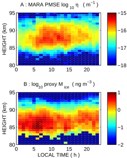
Fig. 7. Panel (A) Daily variation of measured PMSE volume re-flectivity at MARA (median values) from 6 December 2007 to 31 January 2008. Panel (B) proxy for ice mass density calculated from the PMSE reflectivity and background electron density.
and minimum varying between a factor 4 and a factor 10. In Fig. 7 we show the time variations, as a function of height for the most likely values of our model withp=q=1.
Considering IWC in more detail, we can see that our “most likely” proxy slightly underestimates (by about 20%) the amount at 01:00 LT, as compared to the SOFIE measure-ments. A likely cause of this discrepancy can be discerned from the profiles in Fig. 5 where it can be seen that the proxy tends to underestimate the amount of ice at the lowest al-titudes. On average for the whole comparison period, the SOFIE measurements show 28% of the IWC from heights below 84 km, whereas our proxy has only 12% from those heights (at the same LT). The very low electron densities be-low 84 km will tend to make PMSE weak so that they are of-ten below the detection threshold for MARA, and it is likely that this introduces some bias.
[image:8.595.318.535.63.333.2]Diurnal variation of PMC, for rather lower latitudes, 50– 58◦N, have also been reported by Stevens et al. (2009). These show highest PMC occurrence rates 00:00–06:00 LT and lower values 07:00–16:00 LT. The amplitudes of the daily variation are similar in the reported NLC and PMC occurrence rates (a factor 3–10) and in our height averaged proxyMice(about a factor 4). The PMC observations, how-ever, suggest a large secondary maximum at 17:00–18:00 LT which is not seen clearly in either the NLC measurements or in our proxyMice. Stevens et al. (2009) suggest that this may be primarily a transport effect due to meridional trans-port of ice from more polar latitudes by semidiurnal tidal winds. It should be noted, that the NLC observations were sensitive only to the ice particles at the lowest heights (av-erage 82–84 km) covered by PMSE, where ice-particle sizes are largest. The PMC statistics were based on measurements with a detection threshold of 5 ng m−3 and are also biased towards the strongest events. Further, our proxyMice is for a different location – substantially higher latitude and South-ern Hemisphere rather than northSouth-ern. The dominant diurnal tide over Antarctica should modulate PMSE with the same phase as in the Arctic, but the semidiurnal tide is made up of several components which are more variable (Murphy et al., 2006). The amplitude of the diurnal variation in proxyMice will be sensitive to details of the interplay between tidal tem-perature and transport variations which are likely to be both latitude and altitude dependent.
A recent study by Stevens et al. (2010) has used assim-ilation of satellite temperature and water vapour observa-tions into a global numerical model to determine the daily variation of conditions at the summer mesopause. This has been used to drive a microphysical model of PMC forma-tion for the Northern Hemisphere summer of 2007, using IWC measured by SOFIE at 23:00 LT as a constraint to ad-just the parameters of the microphysical modelling. The re-sulting prediction for the daily variation of PMC, in terms of IWC, is similar to our results using the PMSE proxy for the Southern Hemisphere. The model predicts that IWC should be highest between 05:00 and 10:00 LT and lowest between 16:00 and 23:00 LT, with a factor 5–10 between maximum and minimum. The absolute values of IWC predicted (cor-responding to 69◦N latitude) are substantially higher (max-imum 200 µg m−2) than in our “most likely” proxy (maxi-mum 40 µg m−2). However, the IWC measured by SOFIE is also much lower (25 µg m−2) for the Southern Hemisphere period considered here than for the Northern-Hemisphere modelling study (55 µg m−2). This may be an indication of weaker PMC in the Southern Hemisphere. On the other hand, the range of values within the limits of our proxy is large, and peak values as high as 200 µg m−2cannot be ruled out.
As mentioned in connection to Fig. 1, changes in refractive index gradient associated with waves can affect the PMSE reflectivities. In creating our proxyMice we have averaged over 60 days of observations (with about 20% of observa-tions omitted because of moderate or high geomagnetic
dis-turbance levels). This will effectively average out effects of waves with random phase from day to day. There are, how-ever, diurnal and semidiurnal tides which will have similar phase from day to day. Variations associated with tides will not be averaged out and may cause features in the local-time variation of proxyMicewhich are not due in reality to varia-tions in ice mass density. More detailed understanding of the effect of tidal waves on PMSE reflectivity will be needed to be able to assess the contribution of this factor.
Note that median values of volume reflectivity have been used both in deriving our model for proxyMiceby comparing with SOFIE measurements close to 01:00 LT, and in apply-ing that model to find the daily variation. Median volume reflectivities are substantially lower than mean values, as il-lustrated by Fig. 1. In this case, for averages over the whole season, during any particular hour of LT, median volume re-flectivities are lower than means by about a factor 20. Pre-vious estimates of the daily variation of PMSE reflectivity at Wasa/Aboa published in Nilsson et al. (2008) are mean values, and are therofore much higher in numerical value. The diurnal variation in the present data, which represents 2 months of observations during the main PMSE season, is also slightly different from that found in Nilsson et al. (2008), which represented only 16 days of observations, at the end of the previous season. In the present data, minimum reflec-tivities are found around local midnight, rather than around 20:00 LT as found for the end-of season measurements by Nilsson et al. (2008).
6 Conclusions
We have compared PMSE reflectivity profiles from the MARA 54.5 MHz radar in Antarctica, with ice mass density profiles measured by the SOFIE instrument on the AIM satel-lite, for a two month period in Austral summer 2007/2008. All available joint measurements are for the interval 00:00– 02:00 LT. We find that PMSE and ice occupy the same height ranges, with ice detected throughout the height inter-val where PMSE are observed, from 80 km to 95 km altitude. This is the first time a satellite instrument has been shown to measure ice in the upper half of the PMSE layer and strongly supports the idea that PMSE, at all heights, are caused by the presence of ice particles.
For quiet geomagnetic conditions (Ap<15), and profiles averaged over several days, there is a statistically significant correlation between ice mass density and PMSE volume re-flectivity (rcorr=0.4−0.6). For conditions of constant ion-isation rate, the most likely relation is direct proportionality which is consistent with the suggestion of Rapp et al. (2003) that the quantityZNicer2, can be used as a proxy for PMSE, provided thatZ∝r.
density is that which would be caused by solar short-wave ra-diation in the absence of ice particles). Empirically, we find that ice mass density can be estimated from PMSE reflectiv-ities, leading to a proxy for ice mass density proxyMice= (η/AδNe0/δz) or(η/ANe0). The statistical correlation be-tween proxyMice and measured Mice for profiles averaged over several days, is significantly better (rcorr=0.6−0.9) than when electron density (gradient) is ignored (rcorr= 0.4−0.6).
We have used proxyMice=(η/AδNe0/δz) to estimate the diurnal variation of ice mass density from the diurnal variation of PMSE reflectivity. The result shows that ice mass density is likely to be highest in mid-morning (05:00– 07:00 LT) and significantly less at mid-day and in the after-noon. This is in contrast to PMSE which shows consistently high reflectivities from mid-morning to early-afternoon. The IWC at the 05:00–07:00 LT maximum in the daily cycle is higher than the minimum values in the afternoon-evening sector by a factor 4–10. The daily variation of ice mass densi-ties in our proxy is consistent with the few available observa-tions of diurnal variaobserva-tions in NLC and PMC occurrence rates, and with modelling results for IWC for the Northern Hemi-sphere (Stevens et al., 2010). In particular, the modelling re-sults show similar maxima and minima in the mid-morning and evening sectors, respectively, and a factor 5–10 between minimum and maximum. The total IWC, however, is higher by about a factor 2 in the Northern Hemisphere, compared to the present study, both in the SOFIE observations and in the modelled IWC.
Radar observations of PMSE are available from many sites and generally cover all hours of the day. They offer a potentially powerful tool to monitor variations in ice mass density, including diurnal, seasonal and intra-seasonal varia-tions. Further studies will be needed to confirm our results for other sites and for a wider variety of conditions of back-ground electron density. For studies of diurnal variation, the possible effects of tidal modulation on PMSE reflectivities, independent of effects on ice mass density, will also need to be assessed.
Acknowledgements. Measurements with MARA were part of the SWEDARP and FINNARP expeditions to Queen Maud Land, Antarctica in 2007/2008. Funding for the MARA radar was pro-vided by the Wallenberg Foundation, Sweden. The research has otherwise been supported by the Swedish Research Council, with logistical support from Swedish Polar Research Secretariat and Finnish Academy of Science.
Topical Editor C. Jacobi thanks M. Jarvis and another anony-mous referee for their help in evaluating this paper.
References
Bremer, J., Hoffmann, P., Latteck, R., and Singer, W.: Seasonal and long-term variations of PMSE from VHF radar observations at Andenes, Norway, J. Geophys. Res., 108, 8438, doi:10.1029/ 2002JD002369, 2003.
Codrescu, M., Fuller-Rowell, T., Roble, R., and Evans, D.: Medium energy particle precipitation influences on the mesosphere and lower thermosphere., J. Geophys. Res., 102, 19977–19987, 1997.
Fiedler, J., Baumgarten, G., and von Cossart, G.: Mean diur-nal variations of noctilucent clouds during 7 years of lidar observations at ALOMAR, Ann. Geophys., 23, 1175–1181, doi:10.5194/angeo-23-1175-2005, 2005.
Gage, K.: Radar observations of the free atmosphere : structure and dynamics, in: Radar in Meteorology, edited by: Atlas, D., chap. 28a, pp. 534–565, American Meteorological Society, Boston., 1990.
Gordley, L. L., Hervig, M. E., Fish, C., Russell, J. M., Bailey, S., Cook, J., Hansen, S., Shumway, A., Paxton, G., Deaver, L., Mar-shall, T., Burton, J., Magill, B., Brown, C., Thompson, E., and Kemp, J.: The solar occultation for ice experiment, J. Atmos. Solar. Terr. Phys., 71, 300–315, doi:10.1016/j.jastp.2008.07.012, 2009.
Havnes, O.: Polar Mesospheric Summer Echoes (PMSE) overshoot effect due to cycling of artificial heating, J. Geophys. Res., 109, 1–7, 2004.
Hervig, M. E., Gordley, L. L., Stevens, M. H., Russell, J. M., Bai-ley, S. M., and Baumgarten, G.: Interpretation of SOFIE PMC measurements: Cloud identification and derivation of mass den-sity, particle shape, and particle size, J. Atmos. Solar. Terr. Phys., 71, 316–330, doi:10.1016/j.jastp.2008.07.009, 2009.
Hocking, W. K.: Measurement of turbulent energy dissipation rates in the middle atmosphere by radar techniques: A review, Radio Sci., 20, 1403–1422, doi:10.1029/RS020i006p01403, 1985. Hoffmann, P., Rapp, M., Fiedler, J., and Latteck, R.: Influence
of tides and gravity waves on layering processes in the po-lar summer mesopause region, Ann. Geophys., 26, 4013–4022, doi:10.5194/angeo-26-4013-2008, 2008.
Hooper, D. A., Arvelius, J., and Stebel, K.: Retrieval of atmospheric static stability from MST radar return signal power, Ann. Geo-phys., 22, 3781–3788, doi:10.5194/angeo-22-3781-2004, 2004. Jensen, E. J. and Thomas, G. E.: Charging of mesospheric
parti-cles – Implications for electron density and particle coagulation, J. Geophys. Res., 96, 18603–18615, doi:10.1029/91JD01966, 1991.
Kirkwood, S., Wolf, I., Nilsson, H., Dalin, P., Mikhaylova, D., and Belova, E.: Polar mesosphere summer echoes at Wasa,
Antarc-tica (73◦S): First observations and comparison with 68◦N,
Geo-phys. Res. Lett., 34, L15803, doi:10.1029/2007GL030516, 2007. Kirkwood, S., Nilsson, H., Morris, R. J., Klekociuk, A. R., Holdsworth, D. A., and Mitchell, N. J.: A new height for the summer mesopause: Antarctica, December 2007, Geophys. Res. Lett., 35, L23810, doi:10.1029/2008GL035915, 2008.
Lie-Svendsen, Ø., Blix, T. A., Hoppe, U.-P., and Thrane, E. V.: Modeling the plasma response to small-scale aerosol particle per-turbations in the mesopause region., J. Geophys. Res., 108, PMR 9 1–21, 2003.
Morris, R. J., Murphy, D. J., Vincent, R. A., Holdsworth, D. A., Klekociuk, A. R., and Reid, I. M.: Characteristics of the wind, temperature and PMSE field above Davis, Antarctica, J. Atmos. Solar. Terr. Phys., 68, 418–435, doi:10.1016/j.jastp.2005.04.011, 2006.
in-duced by an inertia gravity wave, Radio Sci., 24, 393–406, doi: 10.1029/RS024i003p00393, 1989.
Murphy, D. J., Forbes, J. M., Walterscheid, R. L., Hagan, M. E., Avery, S. K., Aso, T., Fraser, G. J., Fritts, D. C., Jarvis, M. J., McDonald, A. J., Riggin, D. M., Tsutsumi, M., and Vincent, R. A.: A climatology of tides in the Antarctic mesosphere and lower thermosphere, J. Geophys. Res., 111, 23104, doi: 10.1029/2005JD006803, 2006.
Nilsson, H., Kirkwood, S., Morris, R. J., Latteck, R., Klekociuk, A. R., Murphy, D. J., Zecha, M., and Belova, E.: Simultaneous observations of Polar Mesosphere Summer Echoes at two dif-ferent latitudes in Antarctica, Ann. Geophys., 26, 3783–3792, doi:10.5194/angeo-26-3783-2008, 2008.
Osepian, A., Tereschenko, V., Dalin, P., and Kirkwood, S.: The role of atomic oxygen concentration in the ionization balance of the lower ionosphere during solar proton events, Ann. Geophys., 26, 131–143, doi:10.5194/angeo-26-131-2008, 2008.
Rapp, M. and L¨ubken, F.-J.: Polar mesosphere summer echoes (PMSE): Review of observations and current understanding, At-mos. Chem. Phys., 4, 2601–2633, doi:10.5194/acp-4-2601-2004, 2004.
Rapp, M., L¨ubken, F., Hoffmann, P., Latteck, R., Baumgarten, G., and Blix, T. A.: PMSE dependence on aerosol charge number density and aerosol size, J. Geophys. Res., 108, 8441, doi:10. 1029/2002JD002650, 2003.
Rapp, M., Strelnikova, I., Latteck, R., Hoffmann, P., Hoppe, U.-P., H¨aggstr¨om, I., and Rietveld, M. T.: Polar mesosphere summer echoes (PMSE) studied at Bragg wavelengths of 2.8 m, 67 cm, and 16 cm, J. Atmos. Solar Terr. Phys., 70, 947–961, 2008. Russell, J. M., Bailey, S. M., Gordley, L. L., Rusch, D. W., Hor´anyi,
M., Hervig, M. E., Thomas, G. E., Randall, C. E., Siskind, D. E., Stevens, M. H., Summers, M. E., Taylor, M. J., Englert, C. R., Espy, P. J., McClintock, W. E., and Merkel, A. W.: The Aeron-omy of Ice in the Mesosphere (AIM) mission: Overview and early science results, J. Atmos. Solar. Terr. Phys., 71, 289–299, doi:10.1016/j.jastp.2008.08.011, 2009.
Shettle, E. P., DeLand, M. T., Thomas, G. E., and Olivero, J. J.: Long term variations in the frequency of polar mesospheric clouds in the Northern Hemisphere from SBUV, Geophys. Res. Lett., 36, 2803–2806, doi:10.1029/2008GL036048, 2009. Smirnova, M., Belova, E., Kirkwood, S., and Mitchell, N.:
Po-lar mesosphere summer echoes with ESRAD, Kiruna, Sweden : Variations and trends over 1997-2008., J. Atmos. Solar. Terr. Phys., 72, 435–447, 2010.
Smirnova, N., Ogloblina, O., and Vlaskov, V.: Modelling of the lower ionosphere, Pageophys., 127, 353–379, 1988.
Stebel, K., Barabash, V., Kirkwood, S., Siebert, J., and Fricke, K.: Polar mesosphere summer echoes and noctilucent clouds: Simul-taneous and common-volume observations by radar, lidar and CCD camera, Geophys. Res. Lett., 27, 661–664, 2000.
Stevens, M. H., Englert, C. R., Hervig, M., Petelina, S. V., Singer, W., and Nielsen, K.: The diurnal variation of polar mesospheric
cloud frequency near 55◦N observed by SHIMMER, J. Atmos.
Solar. Terr. Phys., 71, 401–407, doi:10.1016/j.jastp.2008.10.009, 2009.
Stevens, M. H., Siskind, D. E., Eckermann, S. D., Coy, L., Mc-Cormack, J. P., Englert, C. R., Hoppel, K. W., Nielsen, K., Kochenash, A. J., Hervig, M. E., Randall, C. E., Lumpe, J., Bai-ley, S. M., Rapp, M., and Hoffmann, P.: Tidally induced varia-tions of PMC altitudes and ice water content using a data assim-ilation system, J. Geophys. Res., doi:10.1029/2009JD013225, in press, 2010.