UNIVERSITY OF TRENTO
Faculty of Mathematical, Physical and Natural Sciences
Physics Department
Ph.D. Thesis in Physics
Computer simulation of Biological Systems
Supervisors: Ph.D. candidate:
Dr. Maurizio Dapor Anna Battisti
Dr. Giovanni Garberoglio
Doctoral School in Physics, XXIV cycle
AUTHOR’S EMAIL ADDRESS: [email protected]
i
Introduction
This thesis investigates two biological systems usingatomistic modellingand molecular dynamics simulation. The work is focused on: (a) the study of the interaction between a segment of a DNA molecule and a functionalized surface; (b) the dynamical modelling of protein tau, an intrinsically disor-dered protein. We briefly describe here the two problems; for their detailed introduction we refer respectively to chapter 4 and chapter 5.
The interest in the study of the adsorption of DNA on functionalized surfaces is related to the considerable effort that in recent years has been devoted in developing technologies for faster and cheaper genome sequenc-ing. In order to sequence a DNA molecule, it has to be extracted from the cell where it is stored (e.g. the blood cells). As a consequence any genomic analysis requires a purification process in order to remove from the DNA molecule proteins, lipids and any other contaminants. The extraction and purification of DNA from biological samples is hence the first step towards an efficient and cheap genome sequencing. Using the chemical and physical properties of DNA it is possible to generate an attractive interaction be-tween this macromolecule and a properly treated surface. Once positioned on the surface, the DNA can be more easily purified. In this work we set up a detailed molecular model of DNA interacting with a surface functionalized with amino silanes. The intent is to investigate the free energy of adsorption of small DNA oligomers as a function of the pH and ionic strength of the solution.
Contents
Introduction. i
I Theory 5
1 Overview of Molecular Modelling 7
1.1 Ab-initio Calculations . . . 9
1.2 Semi-empirical Calculations . . . 10
1.3 Molecular Mechanics . . . 10
1.4 Molecular Simulation . . . 11
2 Atomistic Models and Force Field 13 2.1 Empirical energy functions . . . 13
2.2 Parameterization of empirical force fields . . . 14
2.3 Bonded interaction . . . 15
2.3.1 Bond stretching . . . 15
2.3.2 Harmonic angle potential . . . 16
2.3.3 Torsion potential . . . 17
2.4 Non-bonded interactions . . . 19
2.4.1 Van der Waals interactions . . . 19
2.4.2 Electrostatic interactions . . . 20
2.5 Explicit solvent model: the water parametrization . . . 21
2.5.1 TIP model . . . 22
2.5.2 SPC model . . . 23
2.6 Implicit solvent model . . . 24
2.6.1 Potential of mean force . . . 24
2.6.2 Non-polar free-energy contribution . . . 27
2.6.3 Electrostatic free-energy contribution . . . 28
2.7 Application of the electrostatic continuum to biological systems 28
2.7.1 pH and solute charge . . . 31
2.8 A simple example: the Born model . . . 32
2.9 Generalized Born Model . . . 33
2.10 Biomolecular Force Fields . . . 33
3 Simulation methods 39 3.1 Initial coordinates . . . 39
3.2 Initial velocities . . . 43
3.3 Time step . . . 43
3.4 Thermodynamic Boundary Conditions . . . 44
3.5 Long-range and short-range interactions . . . 45
3.5.1 Continuum electrostatics . . . 46
3.5.2 Discrete and continuum electrostatics . . . 47
3.5.3 Discrete electrostatics . . . 48
3.6 Free energy calculation . . . 50
3.6.1 Metadynamics . . . 52
3.6.2 Umbrella Sampling . . . 55
3.7 Essential Dynamics . . . 59
II Computational Experiments 61 4 Adsorption of DNA oligomers on amine-functionalized sur-face 63 4.1 DNA sequencing and diagnostic tool . . . 63
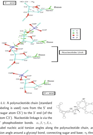
4.2 DNA structure . . . 66
4.2.1 Classical Density Functional Calculations . . . 71
4.3 Molecular dynamics and umbrella sampling calculations . . . 80
4.3.1 Implicit solvent model . . . 81
4.3.2 Explicit solvent model . . . 90
4.3.3 The experiment by the BioSInt group . . . 97
4.4 Discussion and conclusions . . . 100
5 Tau, an intrinsically disordered protein 105 5.1 Intrinsically disordered proteins . . . 105
5.2 The tau protein . . . 106
Contents 3
5.4 The simulation procedure . . . 117
5.5 Domain patterns . . . 118
5.6 SAXS experiment . . . 124
5.7 Selection of equilibrium conformers . . . 125
5.8 Secondary structures . . . 126
5.9 Discussion . . . 128
5.10 Conclusions . . . 133
General conclusion. 136
Acknowledgements 139
Part I
Theory
Chapter 1
Overview of Molecular
Modelling
In this work we use Molecular Modelling to study biological systems on the atomic scale, representing and manipulating the structure of molecules to study properties that are dependent on these three-dimensional struc-tures. Molecular Modelling encompasses quantum mechanics and classical mechanics, and uses minimization procedures, dynamical simulations, con-formational analysis and other computer based methods to understand and predict the behaviour of molecular systems. A first step is the selection of a model to describe the intra- and inter-molecular interactions in the system; these models enable the computation of the energy of any arrangement of the atoms and molecules in the system, and allow to determine how the en-ergy of the system varies with the positions of the atoms. Secondly, one can make a calculation such as an energy minimisation, a Molecular Dynamics (MD) or Monte Carlo (MC) simulation, or a conformational search. Finally, after a check that the calculation has been performed properly (usually a comparison with experimental data) the results can be analysed to calculate specific properties of the system.
The 1950s were very important for the development of this discipline. In this year Watson and Crick discovered the structure of DNA [1]. The deter-mination of its relationship to the biological function of this molecule had a tremendous impact, and was the cornerstone of the paradigm of modern biochemistry and molecular biology. The so-called lock-and-key paradigm established the primary importance of molecular structure for the function of
biological molecules, and the need to investigate this relationship to advance our understanding of the processes of life [2].
The subsequent development of Molecular Modelling was very fast, and gained effectiveness and popularity when computers were introduced in this field, with an improvement in hardware and software tools that is still pro-gressing. In 1963 Ramachandran made one of first experiments that showed the potential of a computational approach in understanding the atomic de-tails of biomolecules: he made a prediction of the allowed conformations of amino acids, the basic building blocks of proteins, using a simple hard-sphere model [3]. With the ever increasing computing power and with faster and ef-ficient numerical algorithms, computational chemistry can be now used very efficiently to solve complex chemical and biological problems. In a compu-tational approach the principal required inputs are: molecular energies and structures, atomic charges, and surface properties. So there is a close con-nection between theory and experiment: computational models evolve as more experimental data become available; biological theories are developed and new experiments are performed, as a result of computational results.
1.1. Ab-initio Calculations 9
1.1
Ab-initio Calculations
The termab-initio refers to computations which are derived from the basic principles of quantum mechanics, such as the Schr¨odinger equation, to de-scribe the motion of electrons and nuclei, with no inclusion of parameters derived from experimental data. Since a complete solution of Schr¨odinger equation cannot be obtained, ab-initio methods are usually mathematical approximations of the full theory, at various levels of accuracy.
The most common type of ab-initio method is the Hartree-Fock (HF) method: by using the variational principle, it can calculate the ground state wave function and ground state energy of a quantum many-body system. The starting point are the spin-orbitals, a set of one-electron wave functions. On these acts the Fock operator, an effective one-electron Hamiltonian op-erator, that takes into account kinetic energy, internuclear repulsion energy, nuclear-electronic Coulomb attraction, and Coulomb repulsion between elec-trons. Inclusion of the latter term, that is considered in a mean-field theory context, is the critical point of the method: neglecting electron correlation can lead to large deviations from experimental results.
Most computations begin with a HF calculation, followed by further cor-rections for the explicit electron-electron repulsion. Among these procedures are the Møller-Plesset perturbation theory (MPn, where n is the order of correction) [4], the Generalized Valence Bond (GVB) [5], the Configuration Interaction (CI) [6], and the Coupled Cluster theory (CC) [7]; these methods are called correlated calculations.
A different method is Quantum Monte Carlo (QMC) [8]. There are sev-eral flavors of QMC, namely variational, diffusion, and Green’s function. These methods work with an explicitly correlated wave-function and eval-uate integrals numerically using a Monte Carlo integration. These calcula-tions can be very time consuming, but they are very accurate.
An alternativeab-initiomethod is the Density Functional Theory (DFT) [9], in which the total energy is expressed in terms of the total electron density rather than through the wave-function.
only to very small systems.
1.2
Semi-empirical Calculations
Semi-empirical calculations have the same general structure as HF, but cer-tain pieces of information, such as two electron integrals, are approximated or completely omitted, to reduce the complexity of the system. In order to correct for the errors introduced by omitting part of the calculation, and to give the best possible agreement with experimental data, the functionals are parameterized. The parameters are determined by fitting the data of a suitable database, entailing either experimental properties or properties derived byab-initio calculations. This method is much faster thanab-initio calculations. On the other hand, if the studied molecule is similar to one found in the database used by the method, the results may be very good; but if the molecule is significantly different from anything in the known set, the results may be very poor. As a matter of fact, semi-empirical calcu-lations have been very successful in the description of organic molecules, where there are only a few different atoms even in large molecules.
1.3
Molecular Mechanics
If a molecule is too complex to use a semi-empirical calculation, it is still possible to model its behaviour totally avoiding an explicit use of a quantum mechanics formalism. The Molecular Mechanics method uses an algebraic expression for the total energy, that consists of simple classical terms. A harmonic oscillator potential may be used to describe the energy associated with bond stretching, valence angle bending, and dihedral rotation; and a classical potential (e.g. Lennard-Jones) may be used to describe intramolec-ular or intermolecintramolec-ular forces, such as Van der Waals interactions. Hydrogen bonds can be defined based on a simple geometric criterium, specified by the maximum hydrogen-donor-acceptor angle and donor-acceptor distance. All parameters in these functions are obtained from experimental data or ab-initio calculations.
1.4. Molecular Simulation 11
of DNA, making it the primary tool of computational biochemistry. The main limit of this method is that there are many chemical process that are not defined within the method (e.g. we cannot consider classical reactions or electronic excitation processes).
1.4
Molecular Simulation
Chapter 2
Atomistic Models and Force
Field
The results that one can obtain in a computational experiment on chemical or physical systems are strictly dependent on the mathematical model used to represent the energy terms that define the interatomic interactions. The quantum mechanics (QM)ab-initio approach is inapplicable to biochemical systems involving macromolecules that contain several thousand atoms, plus their environment due to its very large computational cost. To investigate the systems that are the object of the present study a different approach is necessary, and we have used Molecular Dynamics, implementing force fields defined by the Molecular Mechanics approach.
2.1
Empirical energy functions
Empirical energy functions can fulfill the accuracy and feasibility require-ments of computational studies of biochemical and biophysical systems. The equations of empirical energy functions include relatively simple terms to de-scribe the physical interactions; the atomistic model is used, so that atoms are the smallest particles in the system, rather than electrons and nuclei as in QM. These two simplifying assumptions allow studying structural and dynamical properties of biological molecules, and a very good accuracy can be achieved by optimizing the parameters of the model.
Model Degrees of freedom Some computable prop-erties
Considered Removed
QM nucleus,
electrons
nucleons chemical reactions
Atomistic Force Field
atoms, dipoles electrons interactions,
structural properties Implicit
solvent
solute atoms solvent atoms folding of macro-molecules
2.2
Parameterization of empirical force fields
The empirical energy represents the potential energy V(r) as a function of all the relevant degrees of freedom of a given system. A typical function used in a classical MD code is:
V(r) = X bonds
1
2kbi(bi−b0i)
2+ X
angles 1
2kθi(θi−θ0i)
2
+ X
improper dihedral 1 2k
(idh)
γi (γi−γ0i)
2+ X
dihedrals
k(γdhi )[1 + cos (nγi−δi)]
+ X
atom pairs hCij12
r12 ij −C 6 ij r6 ij + 1 4π qiqj rij i (2.1)
(the symbols introduced here are explained in the next sections).
2.3. Bonded interaction 15
Figure 2.1: Schematic representation of the relevant degrees of freedom.
2.3
Bonded interaction
In reference to Fig. 2.1, which illustrates the most common potential terms between atoms connected by chemical bonds, denoting by ri ={riα} (α = x, y, z) the Cartesian coordinates of thei−th atom, we introduce the fol-lowing parameters:
• the bond distance:
bi =ri+1−ri (i= 1,2, . . . N) ; (2.2)
• the bond angleθi between atoms i, i+ 1 ei+ 2 (i= 1,2, . . . N), that
is between two bonds sharing a common atom:
cosθi =−
bibi+1
bibi+1
; (2.3)
• the torsional angleγi between the plane encompassing atomsi,i+ 1,
i+2 and the plane encompassing atomsi+1,i+2 andi+3. Introducing the normal vectorsξi,ξi+1 to these two planes:
ξi =bi×bi+1 ξi+1 =bi+1×bi+2, (2.4)
γi is defined by:
cosγi=−
ξi
|ξi|
·
ξi+1
|ξi+1|
(2.5)
2.3.1 Bond stretching
Figure 2.2: Behaviours of the two bond stretching interaction C−C [black line] and C=C [red line].
extendible nonlinear elastic (FENE) potential. However, the most common potential used is the harmonic bond potential:
Vs= X
i 1
2kbi(bi−b0i)
2 (2.6)
biandb0i are respectively the distance and the equilibrium distance between two atoms. The parametersb0i are associated with the 3D structure, while the set kbi is characteristic of atoms i and i+ 1, and of the type of bond between them. In Fig. 2.2 the parameterization for C−C and C=C bonds is shown. This example highlights how the same function, with different parameters, can represent the interaction of a pair of atoms with a different type of bonds.
When the potential is known, one can calculate the force acting on the i−th atom:
fi =− ∂Vs ∂ri
=−∂Vs
∂rij rij
ri
=kbi(bi−b0i)
bi
bi (2.7)
2.3.2 Harmonic angle potential
2.3. Bonded interaction 17
Vb = 1
2kθi(θi−θ0i)
2 (2.8)
The forces exchanged between atoms are:
fi =− ∂Vb
∂ri
fk=− ∂Vb ∂rk
fj =−fi−fk (2.9)
The bond-stretching and angle-bending terms are often regarded as ”hard” degrees of freedom because a large energy is required to have a significant deviation from their equilibrium value. Most of the variation in structure of a molecule is thus due to the complex interplay between the torsional and non-bonded contributions, and the knowledge of barriers to rotation around chemical bonds is fundamental to understand the structural properties of the molecule.
2.3.3 Torsion potential
Usually two types of torsion potentials are considered: dihedral angle and improper torsion potentials. The proper dihedral angle depends on the position of four consecutive bonded atoms, whereas the improper dihedral angle depends on the position of four bonded but nonconsecutive atoms.
Proper dihedral
The dihedral angle potential defines the rotation around a bond. This term is oscillatory in nature and requires the use of a sinusoidal function. The parameters included in this term are the force constant kγ, the number of miniman, and the phaseδ.
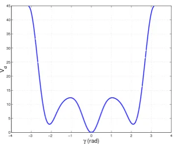
Vdh=kγ(dhi )[1 + cos (nγi−δi)] (2.10)
Figure 2.3: A typical behaviour of a dihedral potential. The parametrization is refered to a butane molecule where the dihedral potential is a sum of five terms
likeVdh.
Improper dihedral
This term is included in order to keep a group in a planar or tetrahedral structure; to represent it a harmonic potential may be used, with only one minimum.
Vidh=kγ(ii−dh)(γi−γ0i)2 (2.11)
γi and γ0i are respectively the dihedral and the equilibrium dihedral angle. The parameters γ0i are associated with the 3D structure, while the setk(γii−dh) is characteristic of atoms involved.
Fig. 2.4 shows the structure of cyclobutane. It is known from experi-mental data that the correct geometry is obtained when atoms 1, 2, 3, and 5 are on one plane as on the right; but without the the improper dihedral term in the force field the system would shift to configuration on the left.
2.4. Non-bonded interactions 19
Figure 2.4: Conformation of cyclobutane corresponding to diffent values of the improper dihedral angle.
2.4
Non-bonded interactions
The non-bonded part of the potential describes interactions between atom pairs that are not covalently bonded to another; solute-solvent, solvent-solvent, solute-ions and solvent-ions interactions are included; fur-thermore the non-bonded term describes the interactions between distant parts of the solute. This term is very important for computational studies of biological systems because the property of macromolecules are strongly influenced by the environment and so the proper treatment of non-bonded interactions is essential for successful biomolecular computations. The mathematical expression of the function referring to these terms can be relatively simple.
2.4.1 Van der Waals interactions
The mathematical function widely used to represent these forces is the Lennard-Jones potential that fulfills the request that v(r) → ∞ at small distances (Pauli exclusion principle), andv(r)→0 as 1/r6for large distances (Van der Waals dispersion).
VLJ = 4ij
σij rij
12
− σij
rij 6
(2.12)
Fig. 2.5 shows the tipical behaviour of the Van der Waals potential, computed for the SPC model of water (described below). The parameters
Figure 2.5: Lennard-Jones potential for SPC model of water.
needed to define this interaction are the well depthij of the potential and the minimum interaction radius σij, defined for every pair of atoms in the system. GROMACS uses an equivalent expressions for the Lennard-Jones function, namely:
VLJ = C
(12) ij r12 ij ! − C (6) ij r6 ij ! (2.13)
The forces acting on the particle are defined by:
fi=− ∂VLJ
∂ri
= 12C
(12)
ij r12
ij
−6C
(6)
ij r6
ij !
fj =−fi (2.14)
2.4.2 Electrostatic interactions
fold-2.5. Explicit solvent model: the water parametrization 21
ing, enzyme activity, binding energies, and of the interactions between a macromolecule and a surface.
The electrostatic interactions are defined by the Coulomb law:
V = 1 4π0
qiqj
rrij (2.15)
where0 is the electric constant andr the relative dielectric constant. The only parameters necessary to define this function are the charges, but in spite of its simplicity the numerical treatement of this term is quite demanding, and it is necessary to use specialized algorithms. We well discuss below of treatment of this term.
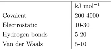
As mentioned before, the equation (2.1) is adequate to treat the physical interactions that occur in biological systems, its accuracy depending on the set of the parameters used.
kJ mol−1
Covalent 200-4000
Electrostatic 10-30
Hydrogen-bonds 5-20
Van der Waals 5-10
Table 2.1: Order of magnitude of the principal interactions involved in the molecular structures.
2.5
Explicit
solvent
model:
the
water
parametrization
An understanding of a wide variety of phenomena concerning biomolecules requires considering solvation effects. In this section we present and discuss the parameterization of water molecules. There are several water models for (bio)molecular simulation. They can be classified in the following way:
• rigid models with a fixed geometry;
• polarizable models that explicitly account for polarization;
• implicit models.
The most used models for biomolecular simulation treat water as a rigid structure: various versions of TIP (Transferable Interaction Potential) and SPC (Simple Point Charge) are available. In Fig. 2.6 we show the general shape of 3-, 4-, 5-, and 6-site water models. The geometric parameters (OH distance and HOH angle) vary depending on the model.
Figure 2.6: Different models of water molecule that correspond to different parametrizations.
2.5.1 TIP model
The TIP series has been developed by William Jorgensen and coworkers [14].
2.5. Explicit solvent model: the water parametrization 23
2.5.2 SPC model
The SPC series has been developed by Herman Berendsen, Wilfred van Gunsteren and coworkers [15]. As for the TIP3P model, all SPC models have 3 interaction sites centered on the atomic nuclei, positive partial charges on the hydrogens and a negative partial charge on the oxygen; the Lennard-Jones parameters are non-zero only for the oxygen.
SPC/E: Extended SPC
This model adds an average polarization correction to the potential energy function:
Epol = 1 2
X
i
(µ−µ0)2
αi
where µ is the dipole of the effectively polarized water molecule (2.53 D), µ0 is the dipole moment of an isolated water molecule (1.85 D from
ex-periments) and αi is an isotropic polarizability constant whose value is 1.68·10−40F m. Since the charges in the model are constant this correction just results in adding 1.25 Kcal/mol (or 5.22 kJ/mol) to the total energy. The SPC/E model is better than the SPC model in reproducing density and diffusion properties [16].
SPC SPC/E TIP3 TIP 4
r(OM) [˚A] - - - 0.15
r(OH) [˚A] 1.0 1.0 0.9572 0.9572
HOH [deg] 109.47 109.47 104.52 104.52
C(12)10−3 [kcal ˚A12mol−1] 629.4 629.4 582.0 600
C(6) [kcal ˚A6mol−1] 625.5 625.5 595.0 610
q(O) -.82 -.8476 -.834
-q(H) +.41 +.4238 +.417 +.52
q(M) - - - -1.04
All MD simulation packages (e.g. GROMACS, CHARMM, AMBER, LAMMPS, GROMOS...) offer the possibility to choose the water model independently of the biomolecular force field. Explicit inclusion of water molecules provides a good representation of the kinetic and thermodynamic properties of the solute molecules. Most biomolecular simulations are made in an all-atoms approximation, using periodic boundary conditions. This yields a large number of water molecules and a considerable increas in the number of degrees of freedom of the system. For this reason and because of the smallness of the time step necessary to integrate the equations of motions (of the order of a femtosecond), the best algorithms can simulate events in the range of 10−9 s to 10−8 s for typical proteins, and 10−6 s for very small
proteins. Many biological processes occur on a larger time scale, therefore much work is aimed at developing alternative models and computationally less expensive approaches.
2.6
Implicit solvent model
In an all-atoms representation of solvated biomoleculs, a large fraction of the overall computational time is used to calculate the detailed trajectories of the solvent molecules. An alternative approach consists in incorporating implicitly the effect of the solvent. The use of a continuum model of the solvent greatly decreases the number of degrees of freedom in the system, and consequently the computing time. Fig. 2.7(a) shows schematically a molecule surrounded by explicit water molecules; Fig. 2.7(b) represents the same biological system but in a medium field that implicitly incorporates the influence of the solvent. This approximation can provide useful quantitative estimates of solvation free energies.
2.6.1 Potential of mean force
In this section we see the statistical approach to the mathematical formula-tion of the implicit solvent model, and we introduce the classical electrostatic equation (CE).
Let us consider a molecule α immersed in a bulk solution β.
2.6. Implicit solvent model 25
(a) (b)
Figure 2.7: Schematical rapresentation of a biomolecule surrounded by explicit water molecules [panel (a)], and in a medium field that implicitly incorporates
the influence of the solvent [panel (b)].
and so one uses a statistical approach to define the probability of a given configuration:
P(X,Y) = exp
−βU(X,Y) R
dXdY exp−βU(X,Y) (2.16)
withβ =1/kBT, kB Boltzmann’s constant and T the equilibrium tempera-ture of the system.
The total potential energy of the systemU(X,Y) can be separated into the following terms:
U(X,Y) =Uα(X) +Uβ(Y) +Uαβ(X,Y) (2.17)
where:
• Uα(X) is the intramolecular potential of the solute;
• Uβ(Y) is the potential representing the solvent-solvent interaction;
• Uαβ(X,Y) is the solute-solvent interaction.
Using P(X,Y) one can calculate every observable of the system as an expected value:
hΘi= Z
If one integrates the function P(X,Y) over the Y coordinate, one can define the reduced probability distribution, depending only on the solute configurations:
P(X) = Z
dYP(X,Y); (2.19)
by introducing (2.16) and (2.17) into (2.19) we have:
P(X) = R
dY exp n
−β h
Uα(X) +Uβ(Y) +Uαβ(X,Y) io
R
dXdY exp n
−β h
Uα(X) +Uβ(Y) +Uαβ(X,Y)
io (2.20)
If one defines a function W(X) such that:
exp{−βW(X)}= Z
dY exp−βU(X,Y) (2.21)
one can write (2.20) in the canonical form for a system in equilibrium at temperatureT:
P(X) = exp
−βW(X) R
dXexp−βW(X). (2.22)
The function W(X) is an effective configuration-dependent free energy, and is called the potential of mean force (PMF); it is a function only of solute configurations, and its gradient is related to the average force:
∂W(X) ∂xi
=h∂U
∂xi
iX =−hFiiX (2.23)
whereh· · ·iX is the average over all solvent coordinates, with the solute in a
fixed configuration specified byX. All solvent effects are included inW(X) and consequently in the reduced probability distributionP(X).
It is instructive to calculate from the equation (2.23) the variation of W(X) between two different solute configurations:
W(X2) =W(X1) +
Z X2
X1
X
i dxi·
∂W(X) ∂xi
=W(X1)−
Z X2
X1
X
i
2.6. Implicit solvent model 27
This relationship clearly shows that the PMF in not simply an average potential energy but represents the reversible work performed by the solute molecule against the average solvent force, and is therefore defined up to an additive constant. Usually, it is rescaled by the solvent-solvent interaction, which still satisfies the normalization condition (2.22) :
exp{−βW(X)}= R
dY exp−βU(X,Y) R
dY exp−βUβ(Y)
(2.25)
In W(X) we have the intramolecular solute potential contribution Uα(X), the solute-solute and solute-solvent interactions. The contribution of the last two terms is due to: (a) a short-range repulsive interaction arising from Pauli’s exclusion principle; (b) the Van der Waals attractive force ing from quantum dispersion; (c) long-range electrostatic interactions aris-ing from a non-uniform charge distribution; (a) and (b) are usually called non-polar interactions. One can consider the following splitting:
Uαβ(X,Y) =Uαβ(np)(X,Y) +Uαβ(elec)(X,Y) (2.26)
that produces a similar separation in the free energy, and is commonly used in biomolecular force fields (e.g. AMBER [17], CHARMM [18] OPLS [19]). This separation leads usally to the following formulation:
W(X) =Uα(X) + ∆W(np)(X) + ∆W(elec)(X) (2.27)
Many methods developed for the simulation of biomolecules use the Sol-vent Accessible Surface Area (SASA) [20] to compute the non-polar free energy contribution ∆W(np)(X). The Poisson-Boltzmann (PB) equation is usually used to compute the electrostatic contribution ∆W(elec)(X). The combination of SASA and PB defines the implicit solvent approach.
2.6.2 Non-polar free-energy contribution
surface. Therefore, in a first approximation, the non-polar free energy can be considered proportional to the number of solvent molecules in the first solvation shell. One assumes that the non-polar free energy contribution is directly related to the SASA
∆W(np)(X) =γAtot(X); (2.28)
γ has the dimension of a surface tension and its value is assigned by match-ing experimental data. Atot(X) is the configuration dependent SASA. The limitations of this model are well studied in the literature [22].
2.6.3 Electrostatic free-energy contribution
In order to describe the electrostatic free energy contribution, it is useful to introduce a parameter λso that if λ= 0 the interactions solute-solvent are absent, and ifλ= 1 the full set of interactions is taken into account. The free energy function has a particularly simple form assumingλas a scaling factor of the solute charge (i.e. Uαβ(elec)(X,Y;λ) = λUαβ(elec)(X,Y) ). One has:
∆W(elec)(X) = Z 1
0
dλhUαβ(elec)iλ. (2.29)
hUαβ(elec)iλ is proportional to λbecause the interaction energy of the
sol-vent is proportional to the charge of solute:
∆W(elec)(X) = Z 1
0
dλX i
qiφrf(xi;λ)≈ 1 2
X
i
qiφrf(xi, λ= 1) (2.30)
φrf(xi, λ= 1) is the field acting on the ith solute atomic charge at the po-sitionxi: it is calledreaction field and represents the electrostatic potential exerted on the solute by the polarized solvent [23].
2.7
Application of the electrostatic continuum to
biological systems
2.7. Application of the electrostatic continuum to biological systems 29
calculate the hydration free energy of spherical ions [24]. Later Kirkwood [25] and Onsager [26] extended Born’s model to study an arbitrary charge distribution inside a spherical cavity.
In this approximation, to study a macromolecule in a solvent one has to solve the Poisson equation to find the reaction field:
∇ ·[(x)∇φ(x)] =−4πρα(x), (2.31)
where φ(x), ρα(x) and(x) are respectively the electrostatic potential, the charge density of the solute, and the position dependent dielectric constant. (x) reflects the reorientation of permanent and induced dipoles under the local electric field. Permanent dipoles occur when the distribution of charge over neighboring atoms is not symmetric: typical examples are peptide bonds and water molecules. In liquid water, the relative freedom of the molecules allows a high dipolar rotation and consequently one finds a high dielectric constant (78.5 at 298 K). In contrast, permanent dipoles in a macromolecule can be considered fixed, and the dielectric constant is much smaller. Experimental and theoretical studies suggest that the average di-electric response of such a solute macromolecule can be approximated with a dipole in the range 2-4; furthermore it has been shown that the use of a single dielectric constant appears to be a reasonable approximation to ac-count for the electronic polarization response of the entire macromolecule. On the other hand, induced dipoles arising from electronic polarization, i.e., from the distortion of electronic clouds immersed in an electric field, give a small contribution of electronic polarization (∼4).
Figure 2.8: Schematic representation of the charge distribution in a protein immersed in a continuum medium; the two groups, the background charges and
the titratable charges, are represented.
implemented in the definition of the force field of a specific system.
When in solution there is a ionic concentration (counterions), one can use the equation (2.31) modified according to the Debye-H¨uckel theory of electrolytes [28]:
∇ ·[(x)∇φ(x)]−κ2(x)(x)φ(x) + 4πρα(x) = 0 (2.32)
where the charge density ρα(x) refers only to the protein charges and the ionic effect is totally contained in the second term of the equation. κ(x), called reciprocal Debye length, is a two-valued function; it assumes the value
κ=
8πe2NAI kBT
1/2
(2.33)
if a point in space is ion-accessible, and zero otherwise. NAis the Avogadro number, e is the proton charge, kB is the Boltzmann constant and the solvent dielectric constant. The ionic strength I of the solution is defined as:
I = 1 2
X
i
cizi2 (2.34)
2.7. Application of the electrostatic continuum to biological systems 31
2.7.1 pH and solute charge
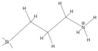
With the simple model in Fig. 2.8 we see that the charges of the protein can be divided into two groups, the background charges and the titrat-able charges. The former are independent of the protonation state of the molecule; the latter represent the charge of the ionic (titratable) residues (Asp, Glu, Lys, Arg, His, Tyr, free Cys, N- and C-terminal), and are gen-erally pH dependent as a consequence of the protonation/deprotonation re-actions.
The pH of the solution is an important parameter, strictly correlated to the electrostatic field. At first glance it would seem a trivial matter to define the charge state of a given group by considering the Henderson-Hasselbach equation of the acid-base equilibrium [29]:
pKa=pH−log f
1−f; (2.35)
f is the degree of protonation, i.e. the fraction of molecules that is proto-nated; pKa is the pH value at which half of the molecules is protonated: its values for the free titratable residues are well known. However, the situation is more complicated because of the other charged sites: the local environment in the protein may shift by several pH units the pKa of a given site from its value typical of the free state. If one defines:
• pKf ree:pKa of a titratable residue in its free state;
• pKint: pKa of a titratable residue in the protein taking the other groups as neutral;
• pKef f: pKaof a titratable residue in the protein taking into account all the charges in the protein;
one finds the following relations [30]:
pKint=pKf ree+ 1 2.3KbT
where ∆Genv is the free energy change when moving the residue from water into the neutral protein;
pKef f =pKint+ 1 2.3KbT
∆Gint (2.37)
∆Gint is the free energy due to the electrostatic contribution of the other charged residues.
The determination of the charge of the titratable residues as a function of the solution pH is a complicated calculation, and some software has been developed for this purpose, e.g. DelPhy (see [31]).
2.8
A simple example: the Born model
For its historical importance and for its simplicity in the following we show the simple Born model, that estimates the free energy of a ion in water. The ion is modelled with a sphere of radiusacentered in the origin characterized by a dielectric constant= 1, whereas the water is modelled by a continuum with a large dielectric constant.
At any pointr, withr > a, for the electric field and for the electrostatic potential we have respectively:
E(r) = q r2
r
r φ(r) = q
r (2.38)
Inside the sphere, for r6= 0, the electric field is given by
E(r) = q r2
r
r . (2.39)
The electrostatic potential atris given by its value on the surface of the ionic sphere plus the work to move, against the field, the charge inside:
φ(r) = q a +
q r −
q
a . (2.40)
If we remove the work required to move the ion from infinity to r in vacuum electrostatic field, we have the work performed by the dielectric medium in moving the ion:
φ(r) =−
1− 1
q
a (2.41)
replacing in equation (2.30) ∆W(elec)(X)≈ 12P
iqiφrf(xi, λ= 1) we arrive to the Born solvation free energy:
∆W(elec) =−1
2
1−1
q2
2.9. Generalized Born Model 33
2.9
Generalized Born Model
In order to take into account the conformational flexibility in the energy minimization of various initial conformations, and in the dynamics, we have to introduce the analytical first derivative of the solvation free energy with respect to the atomic coordinates of the solute. But this calculation is computationally too expensive for large systems. For this reason, it is usual to introduce an approximation to the exact continuum electrostatics, using a semianalytical function expressed as superposition of pairwise additive terms. One of the most popular approximations is the Generalized Born (GB) model [32].
The GB function for the solvation free energy is:
∆Gpol=−1
2
1−e
−κfGB X ij qiqj fGB (2.43)
qi and qj are atomic partial charges and the double sum runs over all pairs of atoms, is the solvent dielectric constant, and κ is the Debye-H¨uckel screening parameter taking the salt concentration into account. fGB is a function that interpolates between an effective Born radius αi, when the distancerij between atoms is short, andrijitself at large distances:
fGB = [rij2 +αiαjexp −r2ij/4αiαj] (2.44)
As we have seen, the effective Born radius αi describes how deeply a charge of a biological system is placed in the low-dielectric medium. It de-pends not only on the intrinsic radius ρi of atomi, but also on the relative positions and intrinsic radii of all other atoms. Several algorithms are avail-able in the biomolecular software to calculate Born radii, e.g. STILL [33], HTC [34], OBC [35].
2.10
Biomolecular Force Fields
we present a list of the most popular force fields used in biomolecular sim-ulations. Each force field has strengths and weaknesses; there isn’t a best one, but one can choose the better one for a particular case. Many studies compare the properties of different force fields [36–38].
AMBER (Assisted Model Building with Energy Refinement)
http://amber.scripps.edu
has been developed since the early 80’s under the leadership of Peter Koll-man at University of California at San Francisco. In Table 2.3 we report the major versions.
CHARMM (Chemistry at Harvard Molecular Mechanics)
http://charmm.org
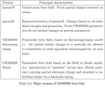
has been developed since the early 80’s under the leadership of Martin Karplus at Harvard University. In Table 2.4 we report the major versions.
GROMOS (Groningen Molecular Simulation)
http://www.igc.ethz.ch/gromos
has been developed since the early 80’s under the leadership of Wilfred van Gunsteren, ETH Zurich. In Table 2.5 we can see the major versions.
OPLS (Optimized Potentials for Liquid Simulation)
http://zarbi.chem.yale.edu
2.10. Biomolecular Force Fields 35
Version Principal characteristic
ff86 United-atom and all atom variants; fixed partial charges cen-tered on atoms.
ff94 Reparametrization, all-atoms force field and fixed partial charges centered on atoms. Charges based on multipole-conformation calculations and a Restrained Electrostatic Potential fit.
ff96 All-atoms force field. Fixed partial charges. Modification of backbone φ, ψ torsional parameters based on ab-initio cal-culations for alanine tetrapeptide.
ff99 All-atoms force field. Fixed partial charges. Minor changes on protein parameters.
ff02 Polarizable variant of ff99. Polarizable dipoles at the atoms, which can be calculated iteratively at each step or prop-agated with the atomic positions as additional dynamical variables. Two variant, with centered point charges and with additional point charges.
ff03 All-atoms force field. Fixed partial charges centered on atoms. Derived from ff99, with charges obtained from ab-initio calculations with a continuum dielectric to mimic sol-vent polarization and new backboneφ, ψ torsional parame-ters.
Version Principal characteristic
param19 United atom force field. Fixed partial charges centered on atoms.
param22 Reparametrization of param19. Charges based onab-initio dimer energies and geometries. Newer CHARMM parameter sets do not include changes in protein parameters.
CHARMM fluctuating-charge
Polarizable force field, based on fluctuating-charge model i.e. the partial atomic charges in a molecule are allowed to redistribute to yield equivalent electronegativity on each atom.
CHARMM Drude
Polarizable force field based on the Shell or Drude model, (i.e. introduction of ”massless” virtual sites /Drude parti-cles) carrying partial electronic charge and attached to in-dividual atoms via a harmonic spring.
Table 2.4: Major versions of CHARMM force field.
Version Principal characteristic
37C4 United-atoms force field. Fixed partial charges centered on atoms.
43A1 Reparametrization of 37C4 using the liquid properties and hydration free energies.
53A6 United-atoms force field (implicit aliphatic H). Fixed par-tial charges centered on atoms. Reppresentation of polar groups based on liquid properties and of side chains based on solvation free energies.
2.10. Biomolecular Force Fields 37
Version Principal characteristic
OPLS United-atoms force field. Fixed partial charges centered on atoms.
OPLS-AA1 Reparametrization of OPLS using liquid properties and hy-dration free energies.
OPLS-AA1 Major reparametrization with special emphasis on torsional parameters.
Chapter 3
Simulation methods
Interest in the dynamics of biomulecular systems derives from its relevance in issues such as folding and unfolding of proteins, the role of dynamics in biological functions, the interaction between proteins or nucleic acids and other systems. Molecular Dynamics (MD) is a useful tool to study many such problems. Using a selected force field, Newton’s equations have to be solved to obtain coordinates and momenta of all atoms of the system along the time trajectory:
mi¨ri=fi i= 1,2. . . N (3.1)
¨
ri = d2ri
dt2 fi=− ∂V(r)
∂ri
(3.2)
ri = (xi, yi, zi), ¨ri andfiare respectively the Cartesian coordinates and the corresponding acceleration of the i−th atom, and the force acting on it. Newton’s law of motion is a second order differential equation that requires two initial values for each degree of freedom to be numerically integrated. To start a simulation one need also of a molecular description (or topology) of the system to be simulated containing information on the system, e.g. which atoms are covalently bonded and other physical information. In Fig. 3.1 there is a simple scheme of a MD computer simulation.
3.1
Initial coordinates
The 3D structures are usually obtained from spectroscopic experiments (e.g, X-ray crystallography, Nuclear magnetic resonance NMR, Electron microscopy EM) [39]. Alternatively, one can use the homology protein
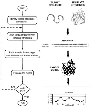
Figure 3.1: The global MD procedure.
structure modelling [41]. Homology modelling, also known as comparative modelling of protein, refers to constructing an atomic-resolution model of thetarget protein from its amino acid sequence and an experimental three-dimensional structure of a related homologous proteins (thetemplates). Ho-mology modelling relies on the identification of one or more known protein structures likely to resemble the structure of the target sequence, and on the production of an alignment that maps residues in the target sequence to residues in the template sequence. It has been shown that protein struc-tures are more conserved than protein sequences amongst homologues, but sequences falling below a 20% sequence identity can have very different struc-ture. We can describe the homology technique with four simple steps, re-peated if needed (Fig. 3.2). For the unknown system (target sequence) we have to:
1. identify related structures with a 3D known structure (template structures);
2. align the target to the template sequence;
3. using information from the template structures to build a model for the target sequence;
3.1. Initial coordinates 41
3.2. Initial velocities 43
3.2
Initial velocities
The velocities are usually taken at random from a standard Maxwellian velocity distribution. For a system in equilibrium at temperature T, one has for a given component of the velocity:
P(v)dv =
m 2πkBT
1/2 exp
− mv
2
2kBT
dv. (3.3)
In order to avoid a thermal schock of the system, one usually starts with a low temperature and increases it gradually by scaling the velocities, allowing the system to relax. This slow heating continues until the simulation reaches the desired temperature.
According to the equipartition theorem, the temperature T(t) is defined by:
T(t) = 1 kBNdof
Ndof X
i=1
mi|vi|2 (3.4)
whereNdof is the number of unconstrained degree of freedom (Ndof = 3N−
n,N is the number of atoms andnis the number of constraints).
3.3
Time step
The most common integration algorithms used in the MD simulation package (e.g. AMBER, CHARMM, GROMACS...) are Verlet and Leap-frog [42].
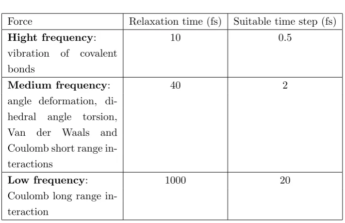
A very important parameter is the integration time step ∆t: a smaller ∆t produces greater accuracy but on the other hand is computationally more expensive; a good choice of the time step yields a good balance between economy and accuracy. The choice of ∆tis correlated to the problem under examination: different types of analysis require different values of the time step. In Tab. 3.1 we give the reference value for some properties.
When the oscillatory frequency of a bond is greater than kBT/~ (~ = h/2π Planck’s constant)1 it is necessary to treat the motion with quantum mechanics and this is true for the vibration of covalent bonds at room tem-perature (see Tab. 3.1). If one is not interested in observables related to the stretching of the chemical bonds, it is customary to fix them to their equi-librium values, using geometrical constraints to keep their length constant. This procedure has two related advantages: it removes the frequencies that
1
Force Relaxation time (fs) Suitable time step (fs)
Hight frequency: 10 0.5
vibration of covalent bonds
Medium frequency: 40 2
angle deformation, di-hedral angle torsion, Van der Waals and Coulomb short range in-teractions
Low frequency: 1000 20
Coulomb long range in-teraction
Table 3.1: Reference values of time steps in different range of frequency.
can not be processed classically, and allows the use of a larger time step with a typical speed up of a factor of∼4.
A number of algorithms have been developed to implement geometrical con-straints, e.g. SHAKE [43], or LINCS [44].
3.4
Thermodynamic Boundary Conditions
A direct solution of Newton’s equations yields trajectories typical of the microcanonical ensemble NVE (where number of atoms, volume and energy of the system are costants), but other algorithms have been developed to generate trajectories in NVT or NPT ensemble (where number of atoms, volume and temperature, or number of atoms, pressure and temperature of the system are kept constant). The latter algorithms are used in particular in biology, where the systems are naturally coupled with a thermal bath.
3.5. Long-range and short-range interactions 45
3.5
Long-range and short-range interactions
As discussed in the previous chapter, a typical potential energy function has the form:
E=Eb+Eθ+Eγ | {z }
bonded
+EV dW +Eel | {z }
nonbonded
(3.5)
where E is the total molecular energy, Eb and Eθ are harmonic terms de-scribing bond and angle vibrations, and Eγ describes the torsion energy (we include in theEγ the proper and the improper dihedral terms); EV dW andEel are nonbonded terms that describe interactions between atom pairs that are not part of a common bond, valence or torsion angle. EV dW takes into account dispersion and repulsion terms, whereas Eel is the Coulomb interaction.
The computer time required to calculate the potential energy of a par-ticular conformation in a large system is dominated by the calculations of the nonbonded interactions. This is due to the number of nonbonded pairs, which is much larger than the number of terms involved in the bond, angle and torsion interactions. In a system of N atoms (104 is a typical num-ber of atoms in a biomolecule) there are about N bond terms and roughly the same number of angle and torsion terms; by contrast, there are N(N2−1) nonbonded pairs: a straightforward calculation is too expensive.
The functional form (see sec. 2.4.1) of EV dW shows that this term de-scribesshort-range interactions. Short-range means that the total potential energy of a given particle i is dominated by interactions with neighboring particles that are closer than some cutoff distancerc, and that the error that results when we ignore interactions with particles at a larger distance can be made arbitrarily small by choosing rc sufficiently large. If the interactions decay rapidly enough, one can evaluate the error by the following expression [42]:
Utot =X i<j
uc(rij) + N ρ
2 Z ∞
rc
dr u(r) 4πr2 (3.6)
whereucis the truncated potential energy function,ρis the average number density, and we have assumed that the radial distribution functiong(r) = 1 forr > rc.
inaccurate. Auffinger and Beveridge discussed the drawback of using simple cutoff in electrostatics [49].
The electrostatic interaction is a very important issue when studying biomolecular systems: (i) from the physical point of view, because there is an increasing evidence that the electrostatic interaction plays a relevant role in folding, conformational stability, enzyme activity, and binding energies as well as in protein-protein interactions; (ii) from the computational point of view, because the evaluation of its contribution to the total energy of the system is so expensive that it is necessary to develop specific approximate algorithms.
In most force fields the atoms of the system are parametrized using partial charges on the atomic sites. When the charges q1, q2. . . qN are at positions r1,r2. . .rN, the electrostatic energy due to the whole system of charges is given by the Coulomb’s equation:
U = 1 2
N X
i=1
qiφ(ri) (3.7)
where:
φ(ri) = X
j6=i qj rij
rij =|ri−rj| (3.8)
If instead of discrete charges, the charge is described by a smooth charge densityρ(x), the the main equation used to model electrostatic interactions is the Poisson’s equation, given by:
∇ ·[(x)∇φ(x)] =−4πρ(x) (3.9)
In a computer experiment the electostatic interactions are treated solving (3.7) or (3.9) depending on the required accuracy and on the boundary condition.
3.5.1 Continuum electrostatics
3.5. Long-range and short-range interactions 47
3.5.2 Discrete and continuum electrostatics
Approximations based on continuum electrostatics, in which the solvent is represented as a featureless dielectric material, are remarkably successful in representing the electrostatic contribution to the solvation free energy. Nev-ertheless sometimes, depending of the problem, a description in which the structural details of the solvent molecules are ignored may not be appropri-ate; e.g. the structure of water is important in the folding process and the creation of secondary structures.
In order to obtain by computer simulation of a finite cluster a statistics similar to that of an infinite system, Belou and Roux have developed an intermediate approach: here one takes into account the solute and a small number of explicit solvent molecules in the vicinity of the solute (a layer of solvent), and represents the influence of the bulk with an effective solvent potential. This approximation follows from a formal separation of the mul-tidimensional configurational integral in the solvent molecules nearest to the solute and the remaining ones.
Even in this approach, in which the number of explicit molecules is very reduced, the evaluation of the electrostatic interaction by means of the Coulomb potential is computationally too expensive, and an approximation is necessary. A first step to solve this problem was the use of the multiple expansion series. To evaluate the Coulomb energy at r, let us consider N charges q1, q2. . . qN at the positions r(k) = {r(αk)} (α = x, y, z) with k= 1,2. . . N, close to the point b={bα}, so that their distances|r(k)−b|
are small compared to |b−r|(see Fig. 3.3).
In the second-order approximation (quadrupole approximation) we have:
N X
i=1
q(i)
|r(i)−r| '
Q
|b−r|−
3
X
α=1
dα(bα−rα)
|b−r|3
+3 2 3 X α=1 3 X β=1
Θαβ(bα−rα)(bβ −rβ)
|b−r|5
−1 2 3 X α=1 Θαα
|b−r|3 (3.10)
whereQ=PN
i=1q(i) is the total charge of the system,dits dipole moment,
withdα = PN
i=1q(i)(r (i)
α −bα), and Θits quadrupole moment, with Θαβ = PN
i=1q(i)(r (i)
α −bα)(r(βi)−bβ) (α, β indicate the Cartesian coordinates). The Fast Multipole Algorithm (FMA) [50], that reduces the cost of the electrostatic calculation to order N for a system of N particles, is based on this approximation. The simulation of a cell containing the solute and the solvent is divided into subcells. At the beginning of the electrostatic calculation, total charge, dipole and quadrupole moments of each subcell are calculated; the potential energy atris calcutated exactly for the charges in the same and in the adjacent subcells, and using the approximation (3.10) for the nonadjacent subcells. The key of FMA algorithm is to consider the more distant charges as grouped into large subcells.
3.5.3 Discrete electrostatics
In the all-atoms approximation all solvent molecules are treated explicitly; the periodic boundary conditions (PBC) are introduced to minimize surface effects and to reproduce the bulk phases with a minimal number of atoms. The simulation cell (for convenience here we consider a cubic cell of side L), containing the solute and the solvent, is considered at the center of an infinite system obtained by replicating the original cell in all directions, in order to mimic the presence of an infinite bulk surrounding the N-particle system (Fig. 3.4). For every particleiat positionri = (xi, yi, zi), there are infinite images at positionsri+nL= (xi+n1L, yi+n2L, zi+n3L), where nis an integer vector. The total potential energy is:
Utot= 1 2
X
i,j,n 0u(|r
3.5. Long-range and short-range interactions 49
Figure 3.4: Schematic representation of periodic boundary conditions.
the prime over the sum indicates that the terms with i = j have to be excluded whenn= 0.
In order to calculate the short-range interactions (e.g. Van der Waals interactions), all intermolecular interactions are usually truncated beyond a certain cutoff distancerc. As seen before, a suitable choice ofrccan yield the desired degree of accuracy.
Ewald sums
The treatment of electrostatic interactions is more complicated; in this case the introduction of a cutoff produces inaccurate results. The Ewald algo-rithm [42, 51] has been developed to treat the electrostatic interactions in an appropriate way. Applied successfully for many years to the simulation of liquids, it is the reference algorithm for macromolecular simulations.
introducing a cutoff; (b) a long-range part defined in the Fourier space, that can be computed using the Poisson equation.
Figure 3.5: (a) Densityρ(1)is the sum of the point charge and of the Gaussian densities. This generates the short-range term. (b) Density ρ(2) equals the Gaussian density with opposite sign, and produces the long-range reciprocal
sum potential.
3.6
Free energy calculation
Free energy, usually expressed as the Helmholtz function F or the Gibbs function G, is perhaps the most important thermodynamic quantity and a central concept in modern studies on biochemical systems: in fact many physical properties relevant from the chemical or biochemical point of view depend directly or indirectly on the free energy of the system. For example, binding constants, association and dissociation constants, and conforma-tional preferences are all related to the difference in free energy between states.
3.6. Free energy calculation 51
free energy, but one can extend all considerations to the Gibbs function. The Helmoltz free energy is defined in thermodynamics as:
F=U−TS (3.12)
where U is the total energy, T the temperature and S the entropy of a sys-tem. From the microscopic point of view, it is a statistical property, which measures the probability of finding a system in a given state. Furthermore, it is a global property that depends on the extent of the phase (or configu-rational) space accessible to the molecular system.
The statistical physics definition of this quantity is the logarithm of the partition functionZ:
F =− 1
βlnZ (3.13)
=− 1
βln Z
e−βH(q,p)dpdq (3.14)
where β = 1/(kBT) (kB denotes the Boltzmann constant), and q and p represent respectively positions and momenta.
To obtain a good estimate of the absolute free energy, in theory one should sample the whole phase space, which is computationally not possible. But in many applications the important quantities are actually the free energy differences between various macroscopic states of the system, rather than the absolute free energy. Free energy differences allow to quantify the relative likelihood of different macroscopic states; each of these states is the collection of all possible microscopic configurations corresponding to the macroscopic parameters, distributed according to the canonical measureµ; the latter is defined as:
µ(dq dp) =Z−1exp [−βH(q, p)]dq dp. (3.15)
of atomistic simulation that can be applied to force a complex system to overcome sampling barriers, classified according to their scope and range of applicabilty; in our work we have usedumbrella sampling andmetadynamics as discussed in the following.
3.6.1 Metadynamics
The metadynamics algorithm works in the following way. One considers a dynamical system, in equilibrium at a temperature T, described by a set of coordinates x and by a potential V(x). The algorithm is based on a dimensional reduction: one is usually interested in exploring the properties of the system as a function of a finite number of collective variables CVs such as some angles, some distances, a coordination number, the potential energy or any explicit function of x, assuming that they provide a good coarse-grained description of the system. The algorithm calculates the probability distribution of the system as a function of one or few of these predefined collective variables. For example, in a chemical reaction one would choose the distance between two atoms that have to form a bond. The dynamics in the space of the chosen CVs is enhanced by a history-dependent potential constructed as a sum of Gaussians centered along the trajectory in the CVs space.
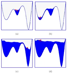
The metadynamics method [52] provides in many cases an efficient frame-work used both for accelerating rare events and for computing the free en-ergy. The method is schematically represented in Fig. 3.6, which shows how it makes the system escape local free energy minima through the lowest free energy saddle point. The same figure illustrates how the method can be used for estimating the free energy.
In the following the capital S is used for denoting CVs as a function of the microscopic coordinatesS(x), while lower casesis used for denoting the value of the CVs.
The equilibrium behaviour of these variables is completely defined by the probability distribution:
P(s) = R exp [−F(s)/T]
3.6. Free energy calculation 53
(a) (b)
(c) (d)
Figure 3.6: The dynamics begins from a minimum of free energy(a). This minimum is quickly filled with Gaussians, and the system evolves through the lowest saddle point in towards a near minimum (b). Afterwards, as the dynamics
continues, the free energy profile is progressively filled with Gaussians (c, d). At the end, the sum of the Gaussians provides the negative image of the free energy.
where F(s) denotes the free energy and is given by:
F(s) =−T ln Z
dxexp
−1
TV(x)
δ[s−S(x)] !
(3.17)
If one generated a very long trajectory x(t), P(s) could be obtained by taking the histogram of the CVs, i.e., at time tone would have:
P(s)∼ 1
t Z t
0
dt0δ s−Sx(t0) (3.18)
regions with very low probability. On the other hand, in metadynamics even if the system is initially at the bottom of a well, the algorithm produces a good sampling by means of the history-dependent potential, that provides an expanding exploration of a progressively larger portion of the configuration space. In the simplest molecular dynamics implementation of this algorithm one introduces a repulsive Gaussian potential everyτG MD steps. Therefore the potential that acts on the system at time tis given by:
VG(S(x), t) =w
X
t0=τG,2τG,... t0<t
exp−[S(x)−s(t
0)]2
2δ2
s
(3.19)
wheres(t) =S(x(t)) are the values of the CVs at timet. The parameters that enter the definition of theVG and influence the accuracy and efficiency of the free energy reconstruction are:
1. the Gaussian height w;
2. the Gaussian widthδs;
3. the frequencyτG by which the Gaussians are added.
If the Gaussians are large, the free energy surface will be explored at a fast pace, but the reconstructed profile will be affected by large errors. Instead, if the Gaussians are small or are placed with low frequency, the reconstruction will be accurate, but it will take a longer time.
The basic assumption of metadynamics is that VG(s, t) as defined in equation (3.19) provides a good estimate of the underlying free energy after a sufficiently long time:
lim
t→∞VG s, t
∼ −F(s) (3.20)
This relation does not derive from any standard identity for the free energy, but was postulated heuristically [53].
Equation (3.20) can be qualitatively understood in the limit of slow de-position, i.e. w→0. In this limit,VG(s, t) varies slowly and the probability of observing sis approximately proportional to
P(s)∝exp − 1
T
F(s) +VG(s, t)
3.6. Free energy calculation 55
If the function F(s) +VG(s, t) has some local minimum, S will be prefer-entially localized in the neighborhood of this minimum, and an increasing number of Gaussians will be added there until this minimum is completely filled. On the other hand, in the region where F(s) =−VG(s, t), the prob-ability distribution will be approximately flat; in this case the corrugations in the free energy are an undesired effect of the number and of the size of the newly added Gaussians.
The efficiency of metadynamics is strongly dependent on the choice of the CVs. In order to obtain a good reconstruction of the free energy, the CVs should describe all the slow events that are relevant to the process of interest; it is also important that all degrees of freedom other than CVs are allowed to relax in the new potential between two depositions of the Gaussians. The CVs should assume clearly distinguishable values in the initial, final, and intermediate states. Finally, it is important to stress that if the number of CVs is too large, it will take a very long time to fill the free energy surface.
A more detailed discussion of the method can be found in Refs. [52, 53].
3.6.2 Umbrella Sampling
The free energy function can be considered as a potential of mean force (PMF) (see section 2.6.1). The concept of potentials of mean force is fre-quently used to characterize the energetics of transitions in solids, fluids, and biomolecular systems. A routinely used technique to compute the PMF along a given reaction coordinateξis the umbrella sampling [54]. This tech-nique aims at overcoming the bias of a limited sampling of energetically unfavorable configurations; it generates a series of initial conditions, each corresponding to a possible state of the system, and confining the simula-tion around this state with an addisimula-tional potential, usually harmonic. In this way one can exlplore very low probability areas of the phase space. The Fig. 3.7 illustrates the method. The steps for this procedure are as follows:
Figure 3.7: Panel (a) illustrates the pulling simulation: a part of the system (blue circle) is pulled away from the rest (red circle). This generates a series of configurations along the reaction coordinate, which in this case is the distance
between the centers of mass of the two parts of the system. These configurations are extracted from the constrained trajectory after the simulation is complete, at points indicated by the dashed arrows. Panel (b) schematizes the independent
simulations within each sampling window, the center of mass of the subsystem being confined in that window by the umbrella biasing potential. Panel (c)
shows the ideal result expected for the histogram of configurations when one uses a harmonic potential; if neighboring windows overlap a continuous energy function can be derived from these simulations.
2. one then extracts from the trajectory produced as in step 1 various frames corresponding to a desired spacing between configurations, as indicated in Fig. 3.7(a) where the dashed arrows point at different positions of the center of mass;
3. a run of the umbrella sampling simulation is started from each config-uration, in which the system is restrained within a window centered on the chosen configurations (Fig. 3.7(b));
3.6. Free energy calculation 57
In this procedure a set of N separate umbrella simulations are carried out, with the usual umbrella potential
wi(ξ) = ki 2
ξ−ξci
2
(3.21)
which restrains the system at positions ξic (i = 1, ..., N) with a force constant ki. From each of the N umbrella simulations an umbrella his-togram is recorded, as in Fig. 3.7(c); it represents the probability dis-tribution Pib(ξ) along the reaction coordinate biased by the umbrella po-tential wi(ξ). We thus obtain a sequence of biased distribution functions P1b(ξ), P2b(ξ),· · ·PNb(ξ), such that P1b(ξ) overlaps with P2b(ξ), P2b(ξ) with P3b(ξ), etc. The unbiased distribution function Pi(ξ) on the ith−window can be written in terms of thePib(ξ):
Pi(ξ) = exp
β wi(ξ)−fi
Pib(ξ) (3.22)
wherefi is the free energy obtained by adding the biasing potential, and is defined by:
exp (−βfi) = Z
dξexp −βwi(ξ)
P(ξ) =hexp −βwi(ξ)
i. (3.23)
The total unbiased probability distribution can be obtained as a linear com-bination of the unbiased probabilities:
P(ξ) = N X
i=1
ci(ξ)Pi(ξ) = N X
i=1
ci(ξ) eβ
wi(ξ)−fi
Pib(ξ) !
. (3.24)
The P(ξ) is related to the PMF via:
W(ξ) =−1
β ln h
P(ξ)/P(ξ0)
i
(3.25)
whereξ0 is an arbitrary reference point, withW(ξ0) set equal to zero.
The weights in theP(ξ) equation are:
ci(ξ) =
nie
−β
wi(ξ)−fi
PN j=1nje
−β
wj(ξ)−fj
(3.26)
and satisfy the normalization conditionPN
The equations (3.24) cannot be solved directly because they contain two unknown quantities: the free energy constants fj and the unbiased distri-bution P(ξ). Therefore, an iterative procedure is necessary; the WHAM equation is: �
![Figure 2.7: Schematical rapresentation of a biomolecule surrounded by explicitwater molecules [panel (a)], and in a medium field that implicitly incorporatesthe influence of the solvent [panel (b)].](https://thumb-us.123doks.com/thumbv2/123dok_us/599888.2059437/31.595.92.456.110.329/schematical-rapresentation-biomolecule-surrounded-explicitwater-implicitly-incorporatesthe-inuence.webp)