978-1-4244-2665-2/08/$25.00 ©2008 IEEE
BYPASSING BIGBACKGROUND: AN EFFICIENT HYBRID BACKGROUND MODELING
ALGORITHM FOR EMBEDDED VIDEO SURVEILLANCE
Brian Valentine, Jee Choi, Senyo Apewokin, Linda Wills, Scott Wills
School of Electrical and Computer Engineering, Georgia Institute of Technology
Atlanta, GA U.S.A.
ABSTRACT
As computer vision algorithms move to embedded platforms within distributed smart camera systems, greater attention must be placed on the efficient use of storage and computational resources. Significant savings can be made in background modeling by identifying large areas that are homogenous in color and sparse in activity. This paper presents a pixel-based background model that identifies such areas, called BigBackground, from a single image frame for fast processing and efficient memory usage. We use a small 15 color palette to identify and represent BigBackground colors. Results on a variety of outdoor and standard test sequences show that our algorithm performs in real-time on an embedded processing platform (the eBox-2300) with reliable background/foreground segmentation accuracy.
Index Terms— Embedded Processors, Color
Clustering, Background Modeling, Multimodal
1. INTRODUCTION
The complexities of observed scenes such as airport/train terminals, traffic intersections, and public events make it impractical to rely solely on human operators for scene monitoring. The availability of low-cost embedded computing platforms and continuing advances in computer vision algorithms have made it practical for designers to consider automated solutions. Many surveillance-based computer vision applications rely on background modeling algorithms to segment foreground from background. This information is used in higher-level tasks such as people tracking, unattended object detection, or anomalous activity recognition. Moreover, in some video surveillance systems, background modeling and foreground detection are the most computationally expensive modules in the system [3]. Since resources on portable-embedded platforms are limited in terms of processor speed, power consumption, and memory capacity, efficient implementations are critical.
Several pixel-based background models continuously maintain color statistics for each pixel [4,17,18,19]. This means that for all frames, every pixel is treated similarly, requiring similar processing overhead and number of
memory accesses. However, long-term stable background data can be represented more compactly and processed faster than new ephemeral foreground data since it remains relatively unchanged.
We present an efficient hybrid background modeling algorithm intended for resource-constrained applications. The algorithm applies to each image pixel, one of two different background modeling techniques, BigBackground (BB) or Multimodal Mean (MMean), depending on whether the pixel is classified as stable versus varying, respectively. Pixels in large, rigid background objects, such as walls of buildings, tree trunks, or sidewalks, will be treated as stable pixels and modeled using a modeling technique called BigBackground. Varying pixels are pixels on multimodal dynamic background elements, such as fluttering leaves, or pixels through which moving foreground objects often pass. These are modeled using an adaptive multimodal technique, called Multimodal Mean [2]. MMean records and maintains, for each pixel, a set of average color values for a small number of background modes the pixel encounters. This set of modes can grow or shrink to allow adaptation of changing pixel values and handling of dynamic background elements, such as rippling waves.
Identifying stable pixels is done using a simple, yet novel technique, based on color clustering within a single initial image, with no prior information of the scene. A storage-efficient color palette is created to represent the BigBackground colors in the large, stable background regions, which account for 47% – 73% of pixels in our test sequences. When using the two techniques, the classification of pixels as stable versus varying is not permanent. Pixels may migrate from one class to another if they frequently fail to match the background model applied to them.
These two backgrounding methods in our hybrid algorithm provide an effective balance between the computational complexities needed for accuracy in adapting new scene elements, with the efficiency achieved by quickly processing large rigid background objects. Our algorithm works well in real-world indoor and outdoor sequences, with substantial speedup, when compared to using only MMean, in sparsely populated scenes.
[6]. The dimensions of the eBox are 115×115×35 mm with a weight of 505g. It contains a Vortex86 SoC-200MHz fanless CPU, with 128MB of onboard SDRAM. It supports up to 2GB of flash memory and is designed for low power consumption (15 Watts). The eBox’s size, weight, and power consumption make it an attractive platform for deployment in a variety of indoor/outdoor conditions. It can be easily and inconspicuously mounted on walls, monitors, poles, etc., and be attached to a USB camera for data collection and processing. Its wireless port can be used to connect to other devices or send processed data to a remote, off-site server. However, the limited memory, storage capabilities, and processor speed of the eBox makes efficient algorithm implementations critical. Our algorithm has been able to achieve real-time performance in real-world test sequences by taking such factors into account in the algorithm design.
This paper is organized as follows. Section 2 contains a discussion of commonly used background modeling algorithms and color clustering algorithms. In section 3 we describe the motivation for BigBackground modeling and its initialization. Section 4 discusses background/foreground segmentation. Section 5 contains descriptions of experiments and discussion of results. Section 6 concludes the discussion.
2. RELATED WORK
Several methods for background/foreground segmentation exist, varying in computational complexity and detection accuracy. Simple techniques include frame differencing and temporal median filters. More complex techniques utilize Gaussian distribution functions or motion analysis. Recent surveys of these can be found in [4,17]. Also, background models can be annotated with temporal information [1,15] to detect new stationary objects or candidate background pixels.
The storage requirements of multimodal background models are large because they retain multiple color values per pixel location, as well as additional values such as weights, variance, means, or observation counts for record keeping. This can require over three times the storage needed to store a single uncompressed image frame, and numerous memory accesses to process data. For example, the storage requirements of the Mixture of Gaussians (MOG) technique [18] are approximately k × 20 bytes per pixel where five 32-bit floating point numbers represent stored weight, variance, and running RGB means. k
represents the number of Gaussians per pixel. If four modes are used, this would make the MOG storage requirements for a 160×120 frame 1.5 MB. This storage requirement, as well as memory accesses, increases proportionally to the number of background modes per pixel location. Since the background is a slowly changing feature within a scene, processing time and memory accesses can be reduced by creating a representation space for commonly seen pixels and keeping their maintenance costs minimal. This can be done by clustering colors belonging to large background regions into a separate representation space, for quick identification and processing.
Data clustering is an unsupervised classification of patterns into groups. It is often used in computer vision to perform color clustering and image segmentation [11]. These include histograms, k-means clustering, octrees, mean shift segmentation, and normalized cuts.
Creating a histogram from the color space is one of the simplest ways of clustering pixel data. The color space can be divided into equally spaced bins with counts incremented depending on the bin to which a pixel belongs. This is fast, as only a single scan through the image is required, and it can be memory efficient, depending on the number of bins used. This technique is also referred to as the popularity method [9].
K-means clustering is another clustering algorithm that can be used to cluster colors [13]. In this algorithm, k number of centroids are defined a priori. Each pixel in the image is matched with its nearest centroid, creating k clusters. Then, barycenters of each cluster are computed, creating a new set of centroids. Each pixel is then re-associated to the new set of centroids until the centroids no longer move. At this stage, a locally-optimal set of color values are said to be found [14].
Octree [8] is a clustering technique that categorizes a color space into groups of branches and leaves. The octree has eight levels that represent the eight bit positions of an RGB color value. Indexing into the octree is performed by grouping bit positions of the pixel’s RGB color components into three-bit words. The top level contains eight child branches each of which could contain a leaf or eight additional child branches. To cluster image colors using octrees, the image is scanned in raster order with each pixel being inserted into its appropriate leaf in the octree. A leaf represents all the pixel values that fall within the bit index ranges ascribed by the octree. The lowest level of the octree, indexed by the LSBs of the RGB pixel value, contains the most detailed grouping of colors. Using the octree for color clustering is advantageous because it can be created quickly and requires a small amount of memory to create and store.
points within each window are computed and the windows are then shifted such that their centers match the computed centroids. This centroid computation and window shifting is repeated until the windows no longer move. Overlapping windows are usually merged.
Normalized cuts in graph theoretic segmentation is more complex, as it involves creating a weighted undirected graph from the pixel data points. The edges that are formed between every pair of pixel points are a function of similarity between the pair. In clustering, the set of points are partitioned into disjoint sets such that a normalized sum of the weights of all the edges connecting a pair of partitions is minimized.
Initially, we experimented with a number of different clustering algorithms, including k-means, octree, and histogram population. A critical difference in our goals compared with traditional clustering methods is that we are interested in identifying and modeling stable regions of pixels, which typically do not completely cover the image. Traditional segmentation methods aim to cluster data so that the entire image is segmented and each segment is mapped to a visually optimal cluster color. Our use of color data clustering is focused on determining the most commonly occurring colors in the image. Interestingly, our experiments with the various clustering methods found that they tend to identify a similar set of commonly occurring colors in a given image. Since the most common colors could be found reliably, independent of the method used, we chose histogram population on which to base the BigBackground clustering method because of its simplicity, fast processing time, and low computational overhead.
3. BIGBACKGROUND
Large objects in a scene are likely permanent, rigid background. Examples of this include roads, sidewalks, buildings, and walls. Depending on the camera’s field of view, these background objects can cover a large percentage of the image frame. Due to the size of these objects, and their relatively homogenous color distributions, it is possible to identify them by finding the most commonly occurring colors in the image. BigBackground colors are stored in a palette and used, in combination with spatial information, to identify stable pixels from a single image frame.
Pixels matching the most common colors in the image are treated as likely belonging to BigBackground objects. Based on an initial image frame, a spatial index map is created to record the location of identified stable pixels and their associated BigBackground color (as an index into the palette). The initialization of the BigBackground model occurs in two steps. The first step scans the initial image to identify the 15 most commonly occurring colors. We found that 15 is sufficient to capture the biggest objects and achieve high coverage of stable regions across the image. The second step takes the initial image and tags pixels
as stable in the index map if they match one of the colors in the palette. Pixels not identified as stable in the initial frame are treated as varying and are processed using the adaptive MMean background modeling algorithm [2].
3.1. BigBackground Palette Generation
Colors associated with BigBackground pixels are stored in a small color palette found using histogram population. The histogram bin is sorted by popularity and the k-most populated color bins and their center values are chosen as the BigBackground colors. The simplicity of initializing and creating a histogram for an image makes this technique very efficient and well-suited for BigBackground processing.
3.2. BigBackground Initialization
The BigBackground color palette is initialized based solely on a single image frame. Using the palette colors, a BigBackground image map is created, identifying all the pixels in the initialization image that match within a threshold, one of the BigBackground colors. The background image map is of size 2Bytes × (rows × cols). For a 160×120 image, 37.5 KB is needed to store the background image map.
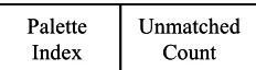
Each element in the image map corresponds to an image pixel and is structured as shown in Figure 2. The Palette Index field contains an index into the BigBackground color palette. Varying pixels, those that are non-BigBackground, are assigned the number zero for the Palette Index field. The Unmatched Count field indicates how many times a BigBackground Color was not matched for a given pixel location in a frame. The purposes of these fields are explained in greater detail in Section 4.
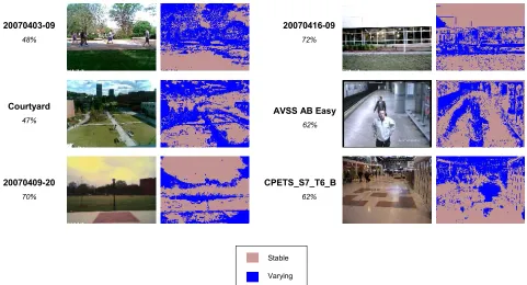
Figure 3 shows several different scenes and their corresponding BigBackground segmentations. The percentage of BigBackground coverage for the initialization frame is also shown. These scenes have a variety of features that present unique challenges to the BigBackground model. 20070403-09 contains fluttering tree leaves which will reduce overall BigBackground coverage. The sequence named Courtyard is captured from a high vantage point, with moving clouds and daytime lighting changes. The CPETS_S7_T6_B sequence has a significant amount of pedestrian traffic. For these scenes, the BigBackground covers from 47% to 73% of the image on average over their entire durations. Efficiently processing and storing the data in the high coverage “stable” BigBackground areas will
Unmatched Count Palette
Index
Unmatched Count Palette
Index
yield significant improvements in execution time and memory accesses.
4. BACKGROUND/FOREGROUND SEGMENTATION
Based solely on the BigBackground image map, pixel locations are identified as being either stable or varying. Stable pixels are processed by the BigBackground modeling algorithm, while varying pixels are processed using the adaptive MMean algorithm. Palette indices in the background image that map from 1-15 indicate that the pixel is stable and its location has a BigBackground color (specified by the palette index) that should be processed using the BigBackground technique. A palette index of 0 indicates that the pixel is varying and does not have a BigBackground color, so the MMean algorithm is used to process the pixel.
4.1. Adaptive Multimodal Mean Modeling
The MMean algorithm, described in detail in [2], does the following. For each pixel location in the image, its current value is compared against a set of background “cells,” representing observed background modes, for that location. Each cell contains a running sum of observed RGB component values, a birth date indicating when the pixel
first was observed, and an observation count. This is illustrated in Figure 4. The fields Rsum, Gsum, Bsum, are the
sum of the individual R, G, B component values that have matched the cell. Rcount1 and Rcount2 are counters used by the MMean cell replacement policy to determine which pixels will be replaced if a new pixel in the current frame is found. The Birth Date field records the frame in which the cell was created and the Count field increments by one each time a new pixel matches the cell.
A pixel is determined to match one of the MMean cells if its color component x is within a predefined threshold of Ej
of one of the cells according to Equation 1:
|I(j,x) - µ(j,x)| ≤ Ej (1)
where I(j,x) is the current image pixel value for color
component j at location x. µ(j,x) is the mean value of color
component j at location x, computed by dividing the running sum of the component by Count. If a match is found, the cell’s observation count value is incremented by one and the current pixel’s RGB component values are added to the cell’s individual RGB component sums. If a match is not found, a new MMean cell is created with the least observed cell being deleted if it falls below a stated cell observation threshold Cth. A pixel is declared foreground if its
observation count is less than the foreground threshold Fth.
Figure 3: BigBackground Initialization
20070403-09 48%
Courtyard 47%
20070409-20 70%
AVSS AB Easy 62%
CPETS_S7_T6_B 62% 20070416-09
72%
Stable
Varying
Sequence Name
Cell counts are periodically decimated, according to a predetermined decimation rate DECRATE, to get rid of unseen cells.
4.2. BigBackground Modeling
BigBackground modeling is performed on stable pixels. The BigBackground color for a stable pixel location is obtained from the color palette and compared against the current pixel using Equation 1. If the current pixel matches the BigBackground color, then it is known that no change has occurred and no further processing is done. This allows the algorithm to quickly skip over stable pixels and focus resources on the areas of the image that feature frequent changes. If the current pixel does not match the BigBackground color, then we know that it has potentially been occluded and the pixel is declared as foreground, with the corresponding Unmatched Count field in the image map incremented by one.
4.3. Changing a Pixel’s Stability Classification
Situations will arise where pixels classified as varying should be migrated to the stable class, and vice versa. For example, a pixel on a moving object may be originally classified as stable because it happened to have a color similar to a large, stable background structure, such as a brick wall. Once the moving object passes by, unless the brick wall is behind the object, the pixel will change to one or more different color values and should be treated as a varying pixel modeled by the adaptive technique. Conversely, an object that moves into a scene and becomes stationary might cause a varying pixel to become stable.
A pixel that is classified as varying should be reclassified as a stable pixel if it satisfies the following conditions:
1. Count ≥ MMWindow
2. MMWindow ≤ Age ≤ (MMWindow + MRange)
3. The cell RGB mean “closely” matches one of the BigBackground palette colors BBcolors according to
Equation 2
|BBcolor(j) - µ(j,x)| ≤ (Ej /3) (2)
where MMWindow is the amount of time a pixel must be seen
before it is considered to be long-term background. The conditions state that a pixel must be old enough (Condition 1), seen frequently enough within a certain age range (Condition 2), and be very close in color value to an existing BigBackground color (Condition 3). Condition 3 contains a
tighter threshold window than the match criteria used in Equation 1. This assures us that pixels which are numerically within the bounds of the threshold, but perceptually different in color, are not declared as stable in the image map.
A pixel that is classified as stable may be reclassified as varying if Equation 3 is true:
UnmatchedCount ≥ BThr×BBWindow (3)
where BBWindow is a small time-block in which stable pixels
are examined for occlusions. BThr is the percentage of the
window that must have unmatched entries for the pixel to be migrated to the varying class. Every BBWindow frames the
UnmatchedCount is reset to zero. If a stable pixel satisfies
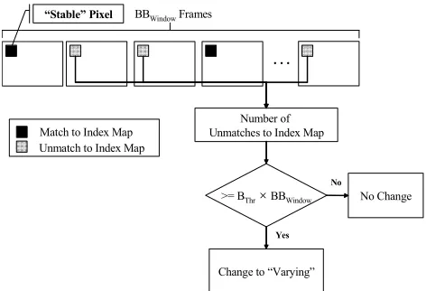
Equation 3, then it signifies that the pixel location has become occluded. The pixel is migrated to the varying class for further examination. This is illustrated in Figure 5.
4.4. BigBackground Illumination Change Adaptation
Illumination changes occur commonly in outdoor scenes due to external factors such as shadows, passing clouds, or simple changes in the time of day. The BigBackground color palette helps adapt to these changes to ensure that the large background regions are processed quickly. This is accomplished by tracking the percentage of BigBackground pixels detected in each frame and looking for large, sustained deviations in BigBackground coverage. A running counter, called COVcount, maintains a recent history of the
number of times the BigBackground coverage has fallen a significant amount below its initial coverage. The BigBackground coverage percentage for the current frame is compared to the coverage of the initialization frame. COVcount is incremented by one if there is a negative
differentiation, BBdev, from the BigBackground coverage
percentage that was computed in the initialization frame. In the opposite case, where there is no significant drop in the Figure 4: MMean Cell Structure
Rcount2 Rcount1
Count Birth Date Bsum Gsum
Rsum Birth Count Rcount1 Rcount2 Date
Bsum Gsum Rsum
Figure 5: Switching Pixel Classification
…
BBWindowFramesNumber of Unmatches to Index Map
>= BThr×BBWindow
“Stable” Pixel
Change to “Varying”
No Change
Yes No Match to Index Map
BigBackground coverage, COVcount is decremented by one,
until COVcount hits zero. If there are several consecutive
frames in which the BigBackground coverage falls, the COVcount will steadily increase. If the BigBackground
coverage percentage remains steady over time, then COVcount
will remain close to or at zero. When COVcount is high
enough, then a lighting change has occurred and the entire BigBackground map is recomputed to adjust for the new environmental conditions.
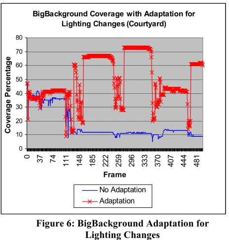
Figure 6 shows a plot of the percentage of BigBackground pixels detected over the entire duration of sequence Courtyard, based solely on the BigBackground colors detected in the first frame. There is a substantial lighting change that occurs within the first twenty frames that causes a sharp drop in BigBackground coverage. From frames 100-150 and 350-450, the intensity from the sun changes dramatically, causing sharp variations between low and bright lighting, and the visibility of shadows cast. The dips in the crossed line of the plot indicate where illumination changes are occurring. Once the color palette has been adjusted to compensate for illumination, the BigBackground coverage reflects the current lighting conditions.
5. EXPERIMENTS AND RESULTS
We have tested our hybrid algorithm on a variety of image sequences. All sequences were resized in resolution to 160x120. The CPETS_S7_T6_B and AVSS AB Easy are standard test sequences used in abandoned baggage detection [16,10]. The CPETS_S7_T6_B and AVSS AB Easy were downsampled in frame-rate to 1fps, for processing on the eBox. Sequences 20070403-09,
20070409-20, and 20070416-09 were captured by graduate students enrolled in an embedded video surveillance course at the Georgia Institute of Technology [20]. Table 1 includes the details for each scene: number of frames processed and ground truth frame number, with all sequences having a starting frame number of zero. The following parameters were used in our experiments, with 4 cells per set used in MMean:
Ej= 30, 15 BigBackground Colors, MMWindow = 25
BBWindow= 10, BThr = 0.7, MRange = 10, BBdev = 5%
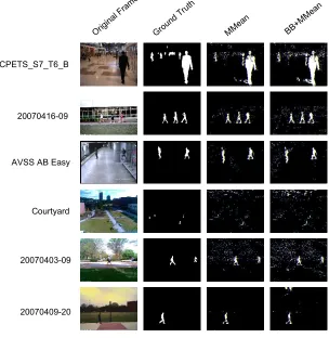
Figure 7 shows the output frames of our algorithm and the ground truth frames in the selected test sequences. Figure 8 shows the false positive/negative errors for each scene.
Table 2 lists the average percentage of pixels that matched BigBackground, as well as the performance of the hybrid BB+MMean algorithm with that of the standalone MMean. Depending on scene activity and environmental conditions (e.g. lighting, weather), the percentage of BigBackground coverage over the scene duration ranged from 47% to 73%.
A detailed analysis in [2] of the performance of MMean in comparison to popular backgrounding techniques, such as MOG, revealed a 6x improvement in MMean’s execution time over MOG on the eBox-2300 platform.
Table 2: Performance Comparison (eBox-2300)
Processing Frame Rates (fps) Sequence (160x120) Average BB Coverage
MMean BB+MMean
20070403-09 47% 34 43
Courtyard 50% 29 42
CPETS_S7_T6_B 60% 35 53
AVSS AB Easy 63% 33 52
20070409-20 71% 36 66
20070416-09 73% 36 69
BigBackground Coverage with Adaptation for Lighting Changes (Courtyard)
0 10 20 30 40 50 60 70 80
0 37 74
1 1 1 1 4 8 1 8 5 2 2 2 2 5 9 2 9 6 3 3 3 3 7 0 4 0 7 4 4 4 4 8 1 Frame C o v e ra g e P e rc e n ta g e No Adaptation Adaptation
Figure 6: BigBackground Adaptation for Lighting Changes 85 600 20070416-09 95 153 20070409-20 55 118
AVSS AB Easy
52 137 CPETS_S7_T6_B 427 499 Courtyard 63 749 20070403-09 Ground Truth Frame Frames Processed Sequence Name (160x120) 85 600 20070416-09 95 153 20070409-20 55 118
AVSS AB Easy
52 137 CPETS_S7_T6_B 427 499 Courtyard 63 749 20070403-09 Ground Truth Frame Frames Processed Sequence Name (160x120)
The hybrid BB+MMean algorithm achieves an average processing speedup of 58% over using just the MMean.
As shown in Figure 7, our algorithm performs particularly well in scenes where the color distributions are homogenous and lighting conditions are stable. Our fastest performing sequences, 20070409-20 and 20070416-09, have these features. Outdoor scenes containing varying lighting conditions and dynamic backgrounds, such as the 20070403-09 and Courtyard sequences, are more challenging. The 20070403-09 sequence contained large trees with fluttering leaves, which caused many of the pixels to be multimodal and therefore processed with the slower, adaptive, MMean technique. In the Courtyard scene, moving clouds and daytime lighting changes required several recomputations of the BigBackground map. In all the scenes tested, 15 colors were adequate in capturing large, stable, BigBackground objects such as tree trunks, roads, walls, and the sky.
6. CONCLUSION
This paper presents a hybrid technique to reduce the processing time devoted to segmenting foreground/ground objects by quickly identifying large stable back-ground regions, and efficiently processing them. A color palette of 15 colors is used to identify colors belonging to the BigBackground objects, while an image map is created to store their spatial locations. Our hybrid algorithm showed an average 58% speedup in processing time over the MMean, while maintaining reasonable accuracy in segmentation. It performs in real-time on an embedded platform with limited processing resources. Since background modeling comprises the most computationally intensive component in many computer vision applications, our technique can be used as an important component in more complex scene analysis.
7. REFERENCES
[1] S. Apewokin, B. Valentine, S. Wills, L. Wills, and A.
Gentile, “Midground object detection in real world video scenes,” IEEE Conf. on Advanced Video and Signal Based Surveillance (AVSS07), September 2007.
[2] S. Apewokin, B. Valentine, S. Wills, L. Wills, and A.
Gentile, “Multimodal Mean Adaptive Backgrounding for
Embedded Real-Time Video Surveillance,” Embedded Computer
Vision Workshop (ECVW07), June 2007.
[3] T.P. Chen, H. Haussecker, A. Bovyrin, R. Belenov, K.
Rodyushkin, A. Kuranov, V. Eruhimov, “Computer Vision Workload Analysis: Case Study of Video Surveillance Systems,” Intel Technology Journal 2005, 9(2): 109-118, 2005.
[4] Cheung, S. and Kamath, C., “Robust techniques for
background subtraction in urban traffic video,” Video Comm. and
Image Processing, Vol. 5308, pp. 881-892, SPIE Electronic
Imaging, San Jose, Jan. 2004.
[5] D. Comaniciu and P. Meer, “Mean shift: A robust approach
toward feature space analysis,” IEEE Transactions on Pattern
Analysis and Machine Intelligence, (5): 603-619, May 2002.
[6] DMP Electronics Inc., “VESA PC eBox-2300 Users Manual,”
September 2006.
[7] K. Fukunaga, Introduction to Statistical Pattern Recognition,
Academic Press, New York, 1972.
[8] M. Gervautz and W. Purgtathofer, “A simple method for color
quantization: octree quantization,” Graphics Gems, Academic
Press Professional, Inc. pp. 287-293, 1990.
[9] P. Heckbert, “Color image quantization for frame buffer
display,” ACM Comput. Graph., vol. 16, no. 3, pp. 297-307, July
1982.
[10]i-Lids dataset for AVSS 2007, Available online at:
www.elec.qmul.ac.uk/staffinfo/andrea/avss2007_d.html.
[11]A. Jain, M. Murty, and P. Flynn, “Data clustering: a review,”
ACM Computing Surveys, 3(31):264-323, 1999.
[12]S. Jianbo, J. Malik, “Normalized cuts and image
segmentation,” IEEE Transactions on Pattern Analysis and
Machine Intelligence, 22(8): 888-905, August 2000.
[13]T. Kanungo, D.M. Mount, N.S. Netanyahu, C.D. Piatko, R.
Silverman, and A.Y. Wu, “An efficient k-Means Clustering
Algorithm: Analysis and Implementation,” IEEE Transactions on
Pattern Analysis and Machine Intelligence, 24(7): 881-892, July 2002.
[14]J.B. MacQueen, "Some Methods for Classification and
Analysis of Multivariate Observations,” Proceedings of 5-th
Berkeley Symposium on Mathematical Statistics and Probability, Berkeley, University of California Press, 1:281-297, 1967.
[15]R. Mathew, Z. Yu, and J. Zhang, “Detecting New Stable
Objects in Surveillance Video,” IEEE Workshop on Multimedia
Signal Processing, pp.1-4, Oct. 2005.
[16]PETS 2006 dataset, Sequence Name S7-T6-B: Video 1,
online: http://www.cvg.rdg.ac.uk/PETS2006/data.html.
[17]M. Piccardi, “Background subtraction techniques: a review,”
IEEE International Conference on Systems, Man and Cybernetics, Vol. 4, pp. 3099-3104, October 2004.
[18]C. Stauffer and W.E.L. Grimson, “Learning Patterns of
Activity Using Real-Time Tracking,” IEEE Transactions on
[19]K. Toyama, J. Krumm, B. Brummitt, and B. Meyers,
“Wallflower: Principles and Practices of Background
Maintenance,” in Proc. of ICCV (1), pp. 255-261, 1999.
[20]S. Wills, L. Wills, “ECE 8893: Embedded Video Surveillance
Systems Projects, Spring 2007,” online:
http://users.ece.gatech.edu:80/~scotty/8893/projects.html
Figure 7: Segmentation Images
BB+M Mea
n
MM ean Gro
und Trut
h
Orig inal
Fra me
CPETS_S7_T6_B
20070416-09
AVSS AB Easy
Courtyard
20070403-09
20070409-20
Figure 8: Error Measurements MMean (160x120)
0 500 1000 1500 2000
CPETS_S7_T6_B 20070416-09 AVSS AB Easy Courtyard 20070403-09 20070409-20
Number of Error Pixels
False Positives False Negatives
BB+MMean (160x120)
0 500 1000 1500 2000
CPETS_S7_T6_B 20070416-09 AVSS AB Easy Courtyard 20070403-09 20070409-20
Number of Error Pixels