Application of Game Theory to Optimize Wireless System Resource Allocation

Application of Game Theory to Optimize

Wireless System Resource Allocation

https://doi.org/10.3991/ijoe.v14i12.8069

Sara Riahi(*₎, Azzedine Riahi Chouaib Doukkali University, El Jadida, Morocco

[email protected]

Abstract—This paper examines the relevance of using game theory in mod-eling and solving some of the problems associated with resource allocation in computer systems.These problems involve many actors who constantly adapt their behavior to their environment. Game theory is used to model the behavior of these actors in order to understand the mechanism of an extended system by studying its performance.It is also used to define strategies and to get an idea of their effectiveness in order to study the consequences of certain events, etc.Game theory as a discipline is commonly listed as a branch of applied mathematics. It is used in various fields.Its objectives are multiple since it involves both capturing and observing behaviors to find out appropriate responses to changes in the en-vironment and also to track patterns of balance in strategic situations where the gain of a player depends on the actions of all others.

Keywords—Game Theory, Nash, MIMO (Multiple Input Multiple Output), Optimization, Allocation, Wireless System.

1

Introduction

generally more efficient than the simple Nash equilibrium. This is due to a shared un-derstanding of information. Competitive algorithms, that is to say, or decisions are se-quentially taken by the players, allowing them to have knowledge of the game of others. This class of games achieves the Stackelberg equilibrium. The penalty concept allows the introduction of secondary utilities to encourage certain behaviors such as reducing the level of interference. The conditions of existence and uniqueness of Nash equilib-rium in the power minimization problem under minimum capacity constraint when sev-eral parallel channels are available. It uses particularly, a distribution of powers in a water-filling for communication[4]. Game theory is generally used in static channels' context and is iterative. Distributed allocations are then made either sequentially or simultaneously. However, in reality, the communication channels evolve over time. This makes use in a very dynamic unfavorable environment.

The rest of the paper is organized as follows: in Part 2 we detail the multi-antenna systems;Part 3 introduces the optimization of wireless systems; Part 4 explains the dif-ferent theoretical approaches; Part 5 gives model and notations used throughout this paper; Part 6 describes the applications of resource allocation problems and methods of allowances; Part 7 is reserved to simulations and analysis of results and conclusions are given in part 8.

2

The multi-antenna systems

Fig. 1. Wireless transmission systems

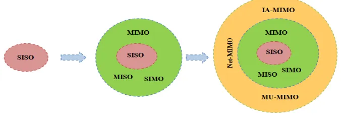
The particularity of MIMO systems is the association with time of the space param-eter in the systematic establishment of the communication. The popularity of researches for this technique is explained by the fact that it has no financial impact on the operation or the acquisition of frequency bands. This is an important section of the business plan. It's more about the hardware and software aspects of a more complex way. The progress of research in this area is critical to there quired speed and quality of the signal received. We can subdivide into two groups: SDM space division multiplexing. The first aims to improve the quality of the received signal and the second increasing the capacity of the link. The combination of both is also possible [8].

Given the inter-symbol interference phenomenon (ISI: Inter-symbol interference) when transmitting at a high rate and the phenomenon of multipath, OFDM technology is a reference solutions. It has been for some time given a special attention.Because, it is shown that it overcomes the limit or cancels the effects related to interference and it also fights the inconvenience caused to Multi-path [9]. It consists of sending serial data simultaneously on subcarrier at a higher speed in a combination of modulation and multiplexing techniques.The combination of MIMO with OFDM is considered a prom-ising solution for increasing the capacity of wireless communication systems and re-sistance to multipath phenomenon.

In this article, we discuss the case of wireless systems. Our concern was to show a comparison in terms of error rates based on different simulation results between some MIMO and SISO gain brought by multi-antenna systems [10]. The channel is consid-ered a non-selective Rayleigh frequency channel and then we expanded the use of space-time codes in the case of frequency-selective channels with OFDM.

2.1 Digital communication system

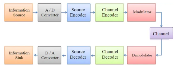
Fig. 3. Block diagram of a digital transmission

Digital transmission of a signal in Figure 3 usually goes through three basic stages. These stages are: the source coding, channel coding and modulation. Source coding is a technique that can compress the information to be transmitted by reducing as much as possible any form of redundancy. Meanwhile,Channel coding is intended to protect the information already compressed against the propagation of disturbances through the transmission medium.It is to replace the information to be transmitted by a message or a code which is less sensitive to noise[6].

The modulation is the third step.Its key role is generally adapting the signal at base-band to the transmission medium by bringing it to a higher frequency. It combines an analog signal to the digital input signal which may comprise one or more bits depending on the desired spectral efficiency. At the reception the inverse process of the emission is monitored. The first step is demodulation and channel decoding that ends by the source decoding [8]. It is easy to show the importance of the channel coding much more than the already compressed message if that is not fully restored and it would be de-graded and lose its content or meaning.

The issue of performance arises and this is reflected in the introduction of control of the longest bit making information. Thus, the channel coding combines size infor-mation , a size code usually larger. This led to the introduction of the concept of return on a channel coder.

The term performance is:

There are two large channel coding categories which are the block coding and con-volution coding. The fundamental difference between these coding categories is at the level of redundancy bits or symbols. They are calculated directly from the bits of infor-mation from the encoder input without considering the precedents in the case of block

K N

K R

codes. On the other hand, during the convolution coding, the coded bits depend both on the preceding bits and on the incoming bits. We will limit our area of interest at the channel coding. To stay within the limits of our theme, we will look precisely at the case of MIMO systems. We do not intend to do a thorough study of the issue, but our concern is limited to an introductory presentation followed by some simulations of space-time codes[8]. STC codes are an increasingly used technique in digital transmis-sion in multiple antenna systems. Indeed, the quality of a link is associated with a max-imum limit of bit error rate (BER). To reduce the BER, we can increase the signal to noise ratio by increasing the power of the transmitted signal. This requires an additional budget of implementation of the appropriate technology that must comply with the laws relating to electromagnetic compatibility and frequency management [11]. The voca-tion of the space-time codes is to increase MIMO system transmission performance by introducing a form of redundancy while keeping bandwidth with a compromise on per-formance. It is useful to make a few reminders on the capacity of MIMO systems.

Capacity. Capacity is defined as the maximum transmission rate which can route a system for a given probability of error.The fundamental theoretical expression limits the capacity for transmission over a MIMO channel. These capabilities increase linearly with the number of antennas in the context of an ideal propagation. This shows the potential of a MIMO channel in terms of spectral efficiency.By appropriate processing, it is possible to reduce a MIMO channel to a set of mono-antennas. On channels, we consider the case of a Rayleigh process for modeling the propagation channel between a transmitting antennas and receiving antennas.We take the case of non-selective MIMO channels in frequency and de-correlated.The capacity of a MIMO system or the channel is known to the receiver and is not known to the sender which increases linearly with the minimum between the number of and receiving transmit antennas [12].

The use of space-time codes in the block reduces overall capacity compared to the optimal value that should reach a MIMO system. The loss of capacity is also related to the level of the channel, the performance of the code and the number of antennas at the reception .The MIMO systems can be used to increase the diversity and the ability of systems, but there is a tradeoff between diversity and Capacity for a particular system. The adverse effects of the correlation between antennas on the earning capacity of multi-antenna systems were also studied.The correlation between antennas causes the change of the distributions of the various sub-channels so that the capacity increases linearly with the minimum number of antennas but with a slope of 10to 20% less strong than for un-correlated channels [11]. In the non-coherent case, the capacity increases linearly with with where designates the period of transmission of a code word.Assuming for the model of the MIMO channel as the power of each transmit antenna to be of , we can estimate the overall channel

ca-pacity, which we denote by C, using the formula of the ability:

(1) n N_t

N n

:

=

min( , )

N N

'(1 '/ )

n -n T n' min( , ,= N Nt r T₂)

T

t P

N

r 2 1

P log 1

²

t

N

t t

C W _s

=

æ ö

= _ç + _÷

è ø

Where symbolizes the bandwidth of each sub-channel, and represents the power received on the i-th sub-channel:

(2)

And is a singular value of the channel matrix denoted . By defining by:

(3) The expression of the capacity by simple algebraic calculations can be in the form:

(4)

Knowing that the non-zero givenvalues of and are the same, the respective values of the capacity of and channel matrix systems are equal. The channel coefficients are random variables. The capacity is expressed as an instan-taneous channel capacity. The mean capacity of the channel is obtained by taking the mean [13].

Considering that and , we find the Shannon formula of the channel capacity:

(5) At high SNR, capacity grows logarithmically with SNR. In a MIMO system, the signal strength received by an antenna is given by:

(6) Where is the power transmitted by an antenna.

Since the rank of is equal to , there is only one signal received in the equivalent MIMO channel model, with the following power:

(7) Thus, by applying the formula, we obtain for this channel configuration the expres-sion of the capacity in the coherent case:

W

l

H

Q

,

,

HH N

N

Q

H H N

N

ì

= í

³

î

!

2 m ²

log det(I )

t

P

C W Q

N

s

= +

H

HH

H H

H

H

1

t r

N

=

N

=

H h

= =

1

2 log (1 )

² P C W s = + 2 ri

P Nt t t

P _{N P}

N = = t P N H

1

(8) In such a system, the order of the diversity gain is R in comparison with the mono-antenna case.

3

Optimizing Wireless Systems

The specificity of wireless systems lies not only in support of communication, elec-tromagnetic waves, including resource management which is critical for performance, but also in user mobility that wireless communications makes it possible[14]. So there are several levels of optimization.

3.1 Wireless communication systems

The wireless term "includes all the networks including at least part of communica-tions ensured by radio links. Wireless communicacommunica-tions offer several advantages over wired communications. First, they allow user mobility, and secondly, their infrastruc-ture is much lighter and faster to deploy. But their capacity is generally lower than that of wired networks. Therefore, wireless links are the critical points in the network, that is to say these are the connections that limit the flow of communications[15]. They constitute what is called the network bottlenecks and their good management depends on network performance. The most famous one is the mobile phone network which is also called cellular network. It includes a variety of technologies such as GSM, UMTS, LTE. But increasingly, cellular networks are used for wired communications applica-tions including web applicaapplica-tions, downloading files and streaming video. The result is a steady increase in observed rates on these networks in recent years [16]. In cellular networks, the wireless part is mainly used to connect users at the heart of the network which is wired, via a base station which we call generically an access point.

Wireless communications are also used for networking, relying exclusively on wire-less links which have no prior infrastructure and allow the topology to change over time .This is called ad hoc networks of mobile which are used in many applications: they allow particularly quickly restore communications after a natural disaster [17].

Electromagnetic waves are the support for wireless communications. Unlike wired connections, electromagnetic waves propagate in all directions if there are no obstacles. Depending on the environment, the wave undergoes several changes mainly due to the phenomena of diffraction, reflection and attenuation. This results in high variability of the signal at a receiver even if it has a fixed location. The phenomenon associated with rapid variations in the signal is called fading, while the one that combines the slow variations is called shadowing and each resulting in a different physical phenome-non[18].

Several resources involved critically in wireless communications: 2

log (1 )

²

r t P

• The frequencies used: in addition to the variability of the signal received from an antenna, several antennas can interfere if they transmit on close frequencies. The capacity of wireless networks is limited by the set of usable frequencies.

• Mobile energy: Wireless communications require more energy than wired commu-nications. Mobile phones are usually small devices with limited battery capacity[10]. This energy must be used wisely.

• The resources of the access point: depending on the used multiplexing technology, resources (frequency, time, or codes) are shared between the various mobiles con-nected to the same access point.

Note that, unlike wired connections, sharing resources degrades the overall perfor-mance. For example, the flow of an access point is a function that is largely based on the number of users.

Mobility. The ability to maintain communication while moving is one of the main advantages of wireless communications. But it also represents a source of difficulty for network management.There are actually two types of mobility. On one hand, there are moving mobiles, and secondly, those who initiate or end a call. Mobility is inherently a random phenomenon that is added, but on a larger time scale, the random fluctuations of the wireless signal.In general, the fine modeling of wireless communication is very complex[8]. In addition to mobility, it is necessary to model the physical system, in particular the signal propagation in a given environment and also the interactions be-tween the different protocols used for communications bebe-tween layers. Added to this is the modeling of different types of applications supported by communications (teleph-ony, data download ...).In this paper, we evaluate the quality of our solutions through simulations on simple models that allow us to analyze the sensitivity of results to certain parameters.

3.2 Control of wireless systems

The connection of a mobile network is the access point that involves firstly the user who decides to make a connection, and also the operator of the access point, which then handles the communication[14]. The operator has different means of action to better satisfy users requests.

User criteria: quality of service. The mobile’s quality of service is a subjective concept which actually depends on the user and the application being used. Often the quality of service includes several criteria[19]. For communications with strong time constraints, such as telephony, the time is paramount.

The criteria of the operators. The goal of operators is to best meet the quality of service of their customers. This involves managing network resources in an effective way[20]. The commonly used performance measures are the average residence time of mobiles, the probability that a mobile cannot connect to the network (due to saturation), or,the probability that the connection of a mobile communication stops. So,this dy-namic criteriais based on time averages.

communications infrastructure [21]. This is done on a large time scale, the result is both a statistical study to anticipate demand and solving complex combinatorial problems to keep the best antennas (and also the frequencies used by the antennas) for the establish-ment of a pricing and differentiated services [19].This is done by choosing an access point for communication with a mobile. Often, a mobile can connect via multiple an-tennas and that choice is managed automatically by the network. This allows distrib-uting the load on all antennas which is a particular form of rodistrib-uting. The management of the choice of the access point is performed for each communication [22] by sharing an access point resources (frequencies, power ...). Resource management is done in the time scale of the transmission of a packet. Note that users can also intervene in the choice of the network to the access point including the choice of technology. The oper-ator must encourage users to act in a manner that is generally effective.

4

Study of approaches

In this article we study the problem of the operator preferences optimization by choosing a mobile communications access point[23]. It is assumed that other means of action (sizing, pricing, resource management) are fixed.

4.1 Dynamic optimization or greedy approach

Optimization of operator preferences can be seen as a dynamic optimization problem with multiple criteria. We worked on dynamic optimization methods with constraints that are based on semi-Markov decision processes. The problem with these methods is that their complexity is exponential in the size of the system and they require knowledge and overall control of the system (the system state in every moment, mobility statistics ...).That's why we have compared them with greedy algorithms which means that these algorithms are based on optimizing a snapshot criterion which does not depend on a centralized controller[24]. We showed that if the system is not overloaded while opti-mizing the overall system throughput at every moment (or at least at each event), it gives nearly optimal performance in terms of average time of mobile phones.For the sake of consistency of the document, these results are not presented here. Nevertheless, we justify the approach that we develop in the following based on the instant optimiza-tion of system performance[25].

4.2 Game theory approach

maximize their quality of service. The performances (instant) system depends solely on the result of the game[26]. The optimization problem of distributed performance is re-flected here by building a game and the implementation of a learning model to show the outcome of the game corresponds to the optimal system performance. The original-ity of our approach is,it jointly considers construction (so-called incentive mechanism) and the apprenticeship model, as well as our knowledge and all items in the field of computing which are based on the theory of games. The typical example is the price of anarchy, in which it is taken for granted that the outcome of the game is Nash equilib-rium. We also take into consideration in the learning models we offer, the possibility of their implementation in real systems. We include in our models random fluctuations that are inherent to wireless networks. In addition, due to the highly decentralized as-pect of networks, it is impossible to ensure perfect synchronization of decision making by users. We also take into account the whole set in the analysis of our models [27].

5

Model and notations

Consider a general system that can be in several states (a way to share communica-tion resources among multiple users, a different routing communicacommunica-tion flow ...). The system status is partly controlled by an operator and by independent entities, which we call the players. The operator and the players have individual preferences when it comes to system status [28]. In general, the preference of the operator is linked to that of the players, for example, if the player preferences are given by values for each state and if the preference of the operator is the sum of these values. The general problem for the operator is to encourage players to act so as to maximize his preference. This requires the construction of an incentive mechanism[29].

The two main difficulties the operator may be facing are that he does not know the preferences of the players, this is called personal preferences, and secondly, it does not control the choice of the final state (but may nevertheless impose penalties).More for-mally, we denote the set of players and the set of states of the system [30]. To avoid problems of mechanisms implementation that we present, we assume that these sets are finished.

5.1 Preferences on the set of states

The operator and the players have preferences on the set of states. These prefer-ences may take the form either of a total order on the states, or (which also implies a total order) a function which associates each states to a value. In the second case, pref-erences are called valuations. We denote by the valuation of the player , and the valuation of the operator [31]. The assessments are therefore functions in . It may be that the operator's evaluation depends on the evaluation of players: if .

In this case, the problem of choosing the state that maximizes V is commonly known problem of social choice. The assessments can represent a monetary value, but also a physical quantity or more abstractly utility. We assume it is consistent to add and com-pare the valuations of the players. In the case of physical quantities, this means that the values are expressed in the same unit. Basically there are two situations: one, in which the preferences of the players are public, that is to say known to the operator, or pref-erences are completely private[32].

5.2 Construction of a mechanism

We stand here in the case of preferences given by valuations. The choice of the state in the set result of a two-step procedure. First, the operator sets the rules of a game, then, knowing the rules of the game, players act accordingly. The given rules of the game define a mechanism that is incentive if the game result is a state that maximizes the evaluation of the operator. We are in the following paragraph on what is meant by outcome of the game [33]. We detail how the game is defined by the operator in a general context. Note, however, that the possibilities of the operator are, according to the situations, subject to restrictions. First, it defines a set of shares for each player. This set does not support a priori any restriction, for example it may be continuous. If denotes the action in chosen by the player , an action profile is the data of an action for each player and is noted .

This belongs to all action profiles observed then, the operator gives a choice function that each action profile, combines state. We denote by this

U x

x

u

v

u

x

!

u u U

V v

Î =

å

x

u S

u

s

u

u U

( )

s

=

s

def u u U

S

S

Î

= ´

:

choice function. Finally, for each player, the operator defines a penalty function , so that the gain of player under the action profile is

(9)

If the penalty is negative ,this means increasing the gain compared to the initial as-sessment of the state that has been selected by the choice function .The penalty function can be interpreted in different ways depending on the application: it can be a money transfer as a virtual quantity transmitted to the players so that they can act on the public interest[34] .We find that the gain function has a public part which is the penalty,and a part that can be private and therefore unknown to the operator , which is . Therefore, the operator does not completely control the player winnings.Finally, the game constructed by the operator is defined by:

The set of players

The sets of actions for each player The gain functions for each player

We must distinguish between the share and the corresponding profile state. From the perspective of the players, what matters is their gain in the game and therefore the profile of action, but from the perspective of the operator it comes to the state. It is assumed here that the penalties imposed on players are not passed on to the operator, only its valuation account is passed[35].

Result of the game: The result of the game is a stock profile of the game. This profile action can be selected in different ways. Either the game is played once and only by one player: the forecast results are difficult in general, except in cases where there are dominant strategies. Either the game is repeated, or in this case, players adjust their action knowing rehearsals of the game.So there is a learning process that must be mod-eled and analyzed. In this case, the result of the game is the profile of actions which is asymptotically selects whether the learning process converges. In all cases, the result of the game depends on assumptions made prior to player behavior.Whether the game is played once or repeatedly, many models of player behavior predict under certain assumptions that the result will be Nash equilibrium. That isa profile action in which no player can win to modify its action unilaterally:

Definition (Nash equilibrium):

The action profile is Nash equilibrium of the game if, for any player and any action _{, we have}

(10)

The classic rating means all players except , and by abuse of notation, we write when we want to distinguish the action of the player (he is not moving from to the first position vector) [33].

:

u

p S

®

!

u

s

( )

( ( ))

( )

u u u

c s

=

v f s

-

p s

u

v

!

f

U

u

S

:

u

c S

®

IR

s

f s

( )

V

s S

Î

( , ,( ) )

U S c

u

u u

s

Î

S

u u

( ,S )

( ' ,S )

u u u u

c S

³

c S

-u

-

u

( , )

s

=

s s

u

u

Note that, Nash equilibrium is not necessarily a stable deviation of two or more play-ers. However, it is assumed that players do not communicate and therefore cannot agree, or in other words form a coalition to jointly increase their gain. Finally note that, in general, there is no reason why the outcome of a game is Nash equilibrium.Firstly, because it does not necessarily exist, and secondly, even if one exists and it is unique, players can earn more by choosing another action.

5.3 Formulation of incentive problem

Finally, the problem of incentive is to construct a set as described above so that the result of the game (or all possible results), be such that the corresponding state maximizes the evaluation of operator. Note that, if there is no constraint on the con-struction of the game, their operator can choose any state by setting

for all .But the operator does not necessarily know the optimal state, especially if it depends on private valuations of the players, or if the complexity makes it impos-sible to calculate [36]. On the other hand, in practical cases that we study later, if the operator chooses but the valuations are private and the set of states and stock profiles coincide, that is to say and the function of choice is , it means that the selected state is the result of the game.

Individual interest against collective interest:

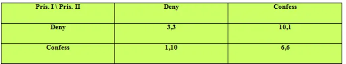
It is quite common that the individual interest does not lead to the choice of a state that maximizes the collective interest. We illustrate this in two classic examples in which . Let’s start with the example of the prisoner’s dilemma. The scenario is as follows;two suspects were arrested and questioned separately. They can either de-nounce one another, or not admit anything. In this game,the collective interest of the suspects is that none of them confess. However, tempting it is, individually,denouncing results in being released [37]. Here, the only Nash equilibrium is a possible outcome of the game (and even dominant strategy as we shall see) is the action profile or the two suspects complain which does not match the collective interest.If neither confesses, then each suspect assessed a minimum prison sentence. If both confess, then they pay the price of an average sentence, and if one complains, then the one who denounced is released while the other gets a heavy sentence (say 10 years).

Table 1. The Prisoners Dilemma

s

f s

( )

V

e

Î

z

f s

( )

=

e

s S

Î

f

S

z = f s( )=s

S

The problem in this example is to find an incentive mechanism to achieve the opti-mum; condition in terms of social cost, by penalizing players based on action.

6

Application to resource allocation problems:

We give two cases of application in resource allocation problems. We assume here that the operator’s valuation is the sum of the evaluations of the players, that is to say

Here, each player must choose one and only one resource among a set.This set is therefore all actions of each player [38]. A state of the system, or equivalently profile of shares, is the association of each pleayer in a single resource. Given a shares in profile m each resource has a load, we note that depends only on players who have chosen this resource[39]. Unlike congestion games , the load is not only the num-ber of players who have chosen this resource , the characteristics of the players being taken into account here,the load is a binary vector such that if has chosen and if not.Finally, assume that the valuation of each player is a function that depends only on the load of the resource he has chosen.If the player has selected the resource , so if , then the evaluation is or is an arbitrary function.Note also that, unlike congestion games, the valuation is a function that can be specific to each player[40].

This particular game models the situation where mobiles have the choice to connect to a cell in a given set of cells. The evaluation of each mobile is a function of the quality of service it gets, the latter being for example flow or delay.To say that the valuation depends only on the load of the cell,it means that one does not take into account inter-ference between different cells. This is justified if the cells are from different technol-ogies or operating on separate frequency bands. In general, the quality of service de-pends not only on the number of online mobile, butalso dede-pends on the characteristics (priority, traffic intensity, to name a few) that are unique to each mobile.

Let denote the profile of actions in the absence of player .The load on each resource in the absence of the player is then written and

.Finally, the choice of the function in

equation gives

(11)

Or is the difference of valuation for the player with-out and with the player .In general it is a negative value for each resource that is

( ) u( )

u U

V s v s

Î =

å

s

( )

l s

r ( )r u Uu

l = l Î lru =1

u

r

0

u

r

s

=

r

u r r

v s d l s=

d

( ,F s-u)

u

u

(0, )

r

l

-( , ) i_i(0, ( ))u

i u s r

v s d l s

-F = _{u( )u i( , )u}

i u

h s- v s

-¹

=

å

( )

( )

( )

( )

u u u u

p s v s V s h s

=

-

+

-,

( )

( )

u i u u

i u

p s

d

s

=

å

, ( ) ( ( , ) ( ))

def

i u s u vi su v si

d _- = F _- -

i

divided into as many parts as the number of players who have chosen. Also note, that is the impact of player on player .

For players who have not chosen the same resource as , the impact is zero, so that .In the end, the penalty function is

(12) We see that the choice of the penalty function, that is to say, this function h, only knows the evaluation of players who have chosen the same resource. The calculation of penalties can take place locally which is a gain in complexity.Take the example of mobile which must attach to cells. This result means that the calculation can be per-formed at each cell. If this were not the case, for example if one makes a choice, it should be that the cells can communicate with each other which is particularly complex if they are not of the same technology.

7

Simulation and analysis of the results

The main objective of the communication systems is to transmit the highest through-put possible with greater reliability. So, the transmission rate is associated with the channel capacity which is represented by a maximum number of data transmitted at any time.The reliability of the transmission, in turn, is associated with the error probability that is inversely related to the ratio signal/noise. To improve throughput and reliability, a simple solution is to increase the transmission power but in a multiuser environment, the power of parallel interference will increase. The second solution is to effectively change the data modulation type but it is necessary to increase the emission spectrum. The latest technique is to use multi-antenna systems that can transmit and receive which improves the reliability and the transmission rate while keeping the same spectrum and the same transmission power.These systems are widely used to MIMO (“Multiple Input Multiple-Output").

In this section, we will start by recalling some results of the game theory that will characterize the capacity of multi-antenna systems. Investigated MIMO channels are characterized by the spatial correlation between the isotopic antennas that are linearly positioned in the antenna arrays for transmission and reception.

For game theory, we can measure the terminal MIMO channel capacities that are expressed as the maximum transmission rate that can be achieved for a low probability of error.We then present the capacity of systems using spatial diversity in reception and transmission in the case where the transmission channel is perfectly known to the re-ceiver but unknown to the transmitter. We will examine the capabilities of both MIMO systems: those of spatial multiplexing MIMO system and those of the MIMO spatial temporal coding. Then, if the issuer knows perfectly the channel status information by the receiver return path, we can maximize the capacity of the MIMO channel or sim-plify the MIMO systems to reduce the complexity and consumption systems.

,

( )

i u

s

d

u

i

u

,

( ) 0

i u

s

d

=

,

( ) ( )

i u

u i u u

i u s s

p s d s

-¹ =

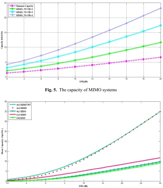
Fig. 5. The capacity of MIMO systems

Fig. 6. Curve capacity vs. SNR for MIMO, MIMO WF, MISO, SISO and SIMO.

The essential purpose of the reception of multi-antenna system is to improve the reliability of the signal through a channel having a high fading. In other words, the spatial diversity reception reduces the effects of fading. In reception, the replies re-ceived from the same, more or less weakened signal on each antenna are combined. Because of the same information replicas, improved reliability at the reception can be obtained. In this section, we examine the ability of various structures of multi-antenna reception systems.Using multiple receiving antennas to fight against the fading chan-nel, the receiver combines the received signals so as to increase the transmission qual-ity.

Gaussian noise (AWGN). We are particularly interested in a transmission system with a carrier frequency 2GHz where a transmitter is fixed but a receiver is moving at a speed of 10 m / s in a randomly given direction.Because, we used a model based on the GSM model, the channel model parameters are: the number of clusters in transmission and reception are equal to 1, broadcasters’ numbers in each cluster are equal to 20, angular dispersions are uniform elevation. We will subsequently use these parameters in the simulations.

Fig. 7. Curve of the outage probability and capability for MIMO, MIMO WF, MISO, SIMO and SISO.

Figure 6 shows the outage capacity with a probability of outage of 10% based on added antennas at reception for some values of the signal to noise ratio. We see that the more SNR is, the more capacity is achieved. The SIMO system has the best perfor-mance among the three techniques studied.However, the use of multiple antennas at the base station in practice is easy to implement and allows to have the same spatial diver-sity gain of reception, provided that the receiver is able to separate the transmitted sig-nals on the same channel. Otherwise, no diversity gain can be obtained.The capacity of the MISO systems increases slightly when some antennas are added in transmission as shown in Fig. 7.The ability approach that of the AWGN channel when the number of transmitting antennas tends to infinity.

Fig. 8. Outage probability comparisons vs SNR for flat fading channels.

The results presented in Fig. 8 illustrate the gains of the capacity of the MIMO sys-tem with WF compared to the MIMO syssys-tem without the WF when the number of re-ception antennas is fixed. We can consider two cases: firstly, and on the other hand, .If , the trend of these results is similar to previous results. At low SNR, the MIMO system with WF can give a significant gain compared to that without the WF. But if the SNR increases, the gain will be reduced.However, in case

, there is a very significant gain. Since the rank of the -channel matrix is , the transmitter will select the best -transmitting antennas and then distribute the power uniformly on each antenna for the WF in the hypothesis of a strong SNR. Otherwise, for the MIMO system without the WF, power is uniformly distributed over antennas. Thus there is a difference between the ergodic capacity of the MIMO channel with WF and the MIMO channel without WF, in case of high SNR.

Fig. 6 shows the capacity of 4x4 MIMO channel correlated with and without the WF based on the distance between the antennas. Due to the appearance of the spatial lation on transmission and in reception, the coefficients of the channel become corre-lated.In the case of low SNR, WF technology always improves the ability even if there is a spatial correlation. However, in the case of a high SNR, the MIMO system with WF can increase the channel capacity when the correlation is very high. This is not the case when the channel is uncorrelated.In recent work, the growth of capacity earnings through the addition of receiver antennas is negligible if the total number of receiving antennas NR is far greater than the number of transmitting antennas.This can be ex-plained by the fact that additional antennas do not provide independent communication channels but only increase the diversity order. Exploiting multiple antennas requires the implementation of multiple RF channels, which are relatively expensive.When it comes to reducing the cost, complexity and consumption of RF channels, many criteria for choosing receiving antennas and transmitting antennas have been proposed to min-imize the probability of error and maxmin-imize capacity limits.

t r

N

£

N

t r

N

!

N

N

£

N

t r

N

!

N

H

min( , )

M

=

N N

M

8

Conclusion

In this paper we study wireless systems in which mobile devices are autonomous in their choice of communication configurations. This independence in decision making may involve, the choice of the access technology to the system, the selection of the access point, the signal modulation, the frequency bands occupied, the power of the transmitted signal, etc.Typically, these configuration choices are made in order to max-imize performance metrics specific to each terminal. Assuming that the terminals take their rational decisions to maximize their performance, game theory applies naturally to model the interactions between the decisions of different terminals.Specifically, the main objective of this article is to study the transmission power balance control strate-gies to satisfy the energy efficiency considerations. The framework for stochastic games is particularly suited to this problem and allows us to characterize the particular achievable performance area for all power control strategies that lead to a state of equi-librium.

9

References

[1]Yang,D., Fang,X., and Xue,G. (2012). Game Theory in Cooperative Communica-tions,IEEE Wireless Communications, 19(2), pp. 44-49. https://doi.org/10.1109/MWC. 2012.6189412

[2]Haykin, S. (2005). Cognitive Radio: Brain-Empowered Wireless Communications, IEEE J. Select. Areas Commun, 23(2): 201–220. https://doi.org/10.1109/JSAC.2004.839380

[3]Oteri, O. (2007). Multiple Antennas and Game Theory", 1-4244-0445-2/07/2007 IEEE,pp.87-90.

[4]Ginde, S. V. (2004). "A game-theoretic analysis of link adaptation in cellular radio net-works" Thesis - Virginia Polytechnic Institute and State University, May 2004.

[5]Arslan,A. Demirkol,M. F. and Song,Y. (2005). Equilibrium efficiency improve-ment in mimo interference systems: A decentralized stream control approach, sub-mitted to, IEEE Transaction on Wireless Communications, 2005.

[6]Sara Riahi, Ali El Hore, Jamal El Kafi, "analysis and simulation of ofdm", IJSR, ISSN Online: 2319-7064, volume 3, Issue 3, Page No (405-409), March 2014.

[7]Sengar,K., Rani,N., Singhal,A., Sharma,D., Verma,S. and Singh,T. (2014). Study and Ca-pacity Evaluation of SISO, MISO and MIMO RF Wireless Communication Sys-tems, Inter-national Journal of Engineering Trends and Technology (IJETT), 9(9): 436-440.

https://doi.org/10.14445/22315381/IJETT-V9P283

[8]Riahi,A. and Riahi,S. (2015). Study of different types of noise and their effects on digital communications,International Journal of Advanced Research in Computer and Communi-cation Engineering, DOI 10.17148/IJARCCE.2015.4968, 4(9): 313-322.

[9]Giri,N. C.,Sahoo,A., Swain,J. R.,Kumar, P.,Nayak,A. andGoswami,P. D. (2014). Ca-pacity & Performance Comparison of SISO and MIMO System for Next Generation Network (NGN), International Journal of Advanced Research in Computer Engi-neering & Technol-ogy (IJARCET), 3(9): 3031-3035.

[11]Riahi,S. Hore,A-EKafi,J-E (2014). Study and Analysis of a Noisy Signal by ViterbiDecod-ing", IJSR, ISSN Online: 2319-7064, 3(10): 392-398.

[12]Halperin,D. Hu,W. Sheth,A. and Wetherall,D. (2010). 802.11 with Multiple An-tennas for Dummies, ACM SIGCOMM Computer Communication Review, 40(1):1-7.

https://doi.org/10.1145/1672308.1672313

[13]Judd,G. Wang,X. and Steenkiste,P. (2008). Efficient channel-aware rate adapta-tion in dy-namic environments", ACM MobiSys,pp. 118–131.

[14]Riahi,S. Hore,A-E, and Kafi,J-E. (2015). Performance study of the OFDM modu-lation for the use in Wireless communication Systems of the 4G, International Re-search Journal of Engineering and Technology (IRJET),2(6):1219-1227.

[15]Hui,H. T. (2009). Influence of antenna characteristics on MIMO systems with compact mon-opole arrays, IEEE Antennas and Wireless Propagation Letters, 8:133-136.

https://doi.org/10.1109/LAWP.2009.2012446

[16]Toyserkani,A. T.,Rydstrom,M., Strom,E. G.and Svensson,A. (A Scheduling Algo-rithm for Minimizing the Packet Error Probability in Clusterized TDMA Net-works", EURASIP Jour-nal on Wireless Communications and Networking, 2009. https://doi.org/10.1155/2009/ 804621

[17]WONG J.K.L., NEVE M.J., SOWERBY K.W. (2002) WIRELESS PERSONAL COMMUNICATIONS SYSTEM PLANNING USING COMBINATORIAL OPTIMISATION. IN: TRANTER W.H., WOERNER B.D., REED J.H., RAPPAPORT T.S., ROBERT M. (EDS) WIRELESS PERSONAL COMMUNICATIONS. THE INTERNATIONAL SERIES IN ENGINEERING AND COMPUTER SCIENCE, 592. SPRINGER, BOSTON, MA

[18]Vorobyov,S. A.,Cui,S., Eldar,Y. C.,Ma,W-K and Utschick,W. (2009). Optimiza-tion Tech-niques in Wireless Communications, EURASIP Journal on Wireless Communications and Networking, 2009. https://doi.org/10.1155/2009/567416

[19]Zhang,H., Fang,Y., Xie,Y., Wu,H. and Guo,Y.(2012). Power control for mul-tipoint coop-erative communication with high-to-low scenario,EURASIP Journal on Wireless Commu-nications and Networking,276. https://doi.org/10.1186/1687-1499-2012-276

[20]Pottie, G. and W. Kaiser, (2000). Wireless Integrated Network Sensors (WINS): Principles and Approach. Communications of the ACM, 43(5):51-58. https://doi.org/10.1145/3328 33.332838

[21]Fakhri,Y., Nsiri, B., Abpitajdine,D. and Vidal,J. (2008). Adaptive Throughput Optimization in Downlink Wireless OFDM System, Computer Science and Com-munications, 1(1): 10-15.

[22]Rappaport,T.S.,Annamalai,A.,Buehrer,R. M. and Tranter,W. H. (2002). Wireless Commu-nications: Past Events and a Future Perspective, IEEE Communications Magazine, 40(5); 148-161. https://doi.org/10.1109/MCOM.2002.1006984

[23]Meng, Y. and Cao,K. (2004) Game-Theory based Multi-Robot Searching Ap-proach, doi=10.1.1.586.5588,2004.

[24]Hespanha,J. P.,Prandini,M. and Sastry,S. (2000). Probabilistic pursuit-evasion games: a one-step Nash approach, 39th conf. on decision and control, https://doi.org/10.1109/CDC. 2000.914136

[25]Daniel, G., Arce, M. and Sandler,T. (2003). An Evolutionary Game Approach to Fundamen-talism and Conflict,159(1): 132-154.

[27]Faigle U. and Peis B. (2008) A Hierarchical Model for Cooperative Games. In: Monien B., Schroeder UP. (eds) Algorithmic Game Theory. SAGT 2008. Lecture Notes in Computer Science, vol 4997. Springer, Berlin, Heidelberg https://doi.org/10.1007/978-3-540-79309-0_21

[28]Marden,J. R.,Ruben,S. D. and Pao,L. Y. (2011). Surveying Game Theoretic Ap-proaches for Wind Farm Optimization, American Institute of Aeronautics and As-tronautics,pp. 1-10. [29]Lee,H. and Baldick, R. (2003). Solving three-player games by the matrix approach with an application to an electric power market. IEEE Transactions on Power Sys-tems, 18(4): 166– 172.

[30]Georges,C. Game Theory Some Notation and Definitions, pp. 1-5.

[31]Seregina, T. (2014). Applications of game theory to distributed routing and delay tolerant networking. Networking and Internet Architecture [cs.NI]. Institut Na-tional des Sciences Appliqu´ees de Toulouse (INSA Toulouse).

[32]Anshelevich E. and Ukkusuri S. (2009) Equilibria in Dynamic Selfish Routing. In: Mavroni-colas M., Papadopoulou V.G. (eds) Algorithmic Game Theory. SAGT 2009. Lecture Notes in Computer Science, vol 5814. Springer, Berlin, Heidelberg https://doi.org/10.1007/978-3-642-04645-2_16

[33]Altman,E. and Kameda, H. (2001). Equilibria for Multiclass Routing in Multi-Agent Net-works. In: 40th IEEE Conference on Decision and Control. Orlando, Florida, USA.

https://doi.org/10.1109/CDC.2001.980170

[34]Chen,Y. (2008). Interactive Networking: Exploiting Network Coding and Game Theory in multiuser wireless communications", Lehigh University, ISBN 1109166796, 9781109166798, ProQuest, Page No (1-68).

[35]Huang,W. (2012). Application of Game Theory in Wireless Communication Networks, The faculty of graduate studies, Electrical and Computer Engineering, The University of British Columbia (Vancouver), pp. 1-160.

[36]Riahi,S., Hore,A-E. and Kafi,J-E. (2016). Optimization of Resource Allocation in Wireless Systems Based on Game Theory", International Journal of Computer Sci-ences and Engi-neering, 4(1): 1-13.

[37]PILLAI.P. S. AND RAO, S. (2016). RESOURCE ALLOCATION IN CLOUD COMPUTING USING THE UNCERTAINTY PRINCIPLE OF GAME THEORY, IEEE SYSTEMS JOURNAL, 10(2): 637- 648 https://doi.org/10.1109/JSYST.2014.2314861

[38]Teng, F., Magoulès, F. (2010) A New Game Theoretical Resource Allocation Al-gorithm for Cloud Computing. In: Bellavista P., Chang RS., Chao HC., Lin SF., Sloot P.M.A. (eds) Advances in Grid and Pervasive Computing. GPC 2010. Lecture Notes in Computer Sci-ence, vol. 6104. Springer, Berlin, Heidelberg,2010. https://doi.org/10.1007/978-3-642-13067-0_35

[39]Xu,X.Yu, H. (2014). A Game Theory Approach to Fair and Efficient Resource Al-location in Cloud Computing, Mathematical Problems in Engineering. https://doi.org/10.1155/2014/ 915878

[40]Joe-Wong, C. Sen,S.,Tian,L. and Mung,C. (2012). Multi-resource allocation: fair-ness-effi-ciency tradeoffs in a unifying framework, in Proceedings of the Annual Joint Conference of the IEEE Computer and Communications Societies (IEEE INFOCOM '12), pp. 1206–1214.

10

Authors

of Sciences, Chouaib Doukkali, El Jadida, Morocco. She is currently PhD in the De-partment of Mathematics and Computer Science, Faculty of Sciences, Chouaib Douk-kali, El Jadida, Morocco. Her research activities focus on the modelling databases, Big-Data, Optimisation, Dataminig, computer protocols, wireless communication, large-scale multimedia systems, mobile applications.

Professor Azzedine Riahi received his PhD in Nuclear Physics in 1987 CENBG at the University of Bordeaux, France, he graduated in Nuclear Medicine, he is a professor the upper education at university chouaib Doukkali since 1988, he is currently Director of laboratory Instrumentation, measurement and control (IMC).