A global model of the ionospheric F2 peak height based on EOF analysis

www.ann-geophys.net/27/3203/2009/

© Author(s) 2009. This work is distributed under the Creative Commons Attribution 3.0 License.

Annales

Geophysicae

A global model of the ionospheric F2 peak height based on

EOF analysis

M.-L. Zhang, C. Liu, W. Wan, L. Liu, and B. Ning

Beijing National Observatory of Space Environment, Institute of Geology and Geophysics, Chinese Academy of Sciences, Beijing 100029, China

Received: 20 October 2008 – Revised: 26 June 2009 – Accepted: 9 July 2009 – Published: 14 August 2009

Abstract. The ionospheric F2 peak height hmF2 is an impor-tant parameter that is much needed in ionospheric research and practical applications. In this paper, an attempt is made to develop a global model of hmF2. The hmF2 data, used to construct the global model, are converted from the monthly median hourly values of the ionospheric propagation factor M(3000)F2 observed by ionosondes/digisondes distributed globally, based on the strong anti-correlation existed between hmF2 and M(3000)F2. The empirical orthogonal function (EOF) analysis method, combined with harmonic function and regression analysis, is used to construct the model. The technique used in the global modelling involves two layers of EOF analysis of the dataset. The first layer EOF anal-ysis is applied to the hmF2 dataset which decomposed the dataset into a series of orthogonal functions (EOF base func-tions) Ek and their associated EOF coefficients Pk. The

base functionsEk represent the intrinsic characteristic

vari-ations of the dataset with the modified dip latitude and lo-cal time, the coefficientsPk represents the variations of the

dataset with the universal time, season as well as solar cy-cle activity levels. The second layer EOF analysis is applied to the EOF coefficients Pk obtained in the first layer EOF

analysis. The coefficientsAk, obtained in the second layer

EOF analysis, are then modelled with the harmonic func-tions representing the seasonal (annual and semi-annual) and solar cycle variations, with their amplitudes changing with the F10.7 index, a proxy of the solar activity level. Thus,

the constructed global model incorporates the geographical location, diurnal, seasonal as well as solar cycle variations of hmF2 through the combination of EOF analysis and the harmonic function expressions of the associated EOF coef-ficients. Comparisons between the model results and obser-vational data were consistent, indicating that the modelling

Correspondence to: M.-L. Zhang ([email protected])

technique used is very promising when used to construct the global model of hmF2 and it has the potential of being used for the global modelling/mapping of other ionospheric parameters. Statistical analysis on model-data comparison showed that our constructed model of hmF2, based on the EOF expansion method, compares better with the observa-tional data than the model currently used in the Internaobserva-tional Reference Ionosphere (IRI) model.

Keywords. Ionosphere (Equatorial ionosphere; Mid-latitude ionosphere; Modelling and forecasting)

1 Introduction

Ionospheric modelling has been one of the leading ways to study the ionosphere. An ionospheric model can be either a theoretical model (also named physical model or first princi-ple model) which is derived from various laws of physics and based on the numerical solution of the equations describing the spatial and temporal distribution of medium parameters or an empirical (or semi-empirical) model which is derived from the observational results. Empirical ionospheric mod-els are not only important for ionospheric research, but also very useful and much needed in a wide range of practical applications, such as radio and telecommunication, satellite tracking, Earth observation from space, etc.

density has its maximum values in the F2 layer, this layer is the most important region of the ionosphere which is pri-marily responsible for the reflection of radio waves in high-frequency communication and broadcasting. For this reason, F2 peak is the key anchor point to determine the ionospheric electron density profiles. Therefore, the F2 layer peak height hmF2 is one of the most important parameters in ionospheric empirical modelling. Due to the lack of observational data of hmF2, in practice, people usually obtained hmF2 based on its strong anti-correlations with the ionospheric propagation fac-tor M(3000)F2 whose value is provided usually by the CCIR (International Radio Consultative Committee) or now called ITU (International Telecommunication Union) M(3000)F2 model (CCIR report, 1967). The CCIR M(3000)F2 model predicts M(3000)F2 based on the 12-month running aver-age sunspot number Rz12, then hmF2 is calculated based on this CCIR M(3000)F2 model values using Eqs. (1–6) listed in Sect. 2. However, recently some authors (Adeniyi et al., 2003; Obrou et al., 2003; Zhang et al., 2004; 2007) found that in the equatorial and low-latitude regions, the val-ues of hmF2 converted from the CCIR M(3000)F2 model value using Eqs. (1–6) have remarkable discrepancies with the observational hmF2. They revealed that the discrepancies stemmed from the inaccuracy of CCIR M(3000)F2 model. Because when the measured M(3000)F2 values are used, the hmF2 converted using Eqs. (1–6) agrees very well with the observational result derived from the manually edited traces of ionograms using ionogram inversion programs. There-fore, there is a necessity to update the existing M(3000)F2 model or construct directly a global model of hmF2. This is an urgent main task of the IRI working group community. To this goal, recently, some new modeling techniques have been proposed to model these parameters. For example, Oyeyemi et al. (2007) proposed a new modelling technique based on the application of neural network to model the M(3000)F2 parameter, whereas Liu et al. (2008) attempted to model the M(3000)F2 parameter based on the empirical orthogonal function (EOF) analysis of the observational dataset. Fur-thermore, recently Gulyaeva et al. (2008) derived a numeri-cal model of hmF2 from the topside database of about 90 000 electron density profile provided by ISIS1, ISIS2, IK19 and Cosmos-1809 satellites for the period of 1969–1987. In this paper, we pursue constructing a global model of hmF2 using a modelling technique which is based on the empirical or-thogonal function (EOF) decomposition of the global hmF2 dataset and the modelling of its associated EOF coefficients. In the following sections, we will first mention the dataset used for our model construction in Sect. 2, and then in Sect. 3 we will describe the modelling technique used. The mod-elling results with some discussions will be shown in Sect. 4 and the last section (Sect. 5) is the summary and conclusion.

2 Data and transformation equations

The fact that hmF2 is a parameter which is not easy to obtain from measurement makes it difficulty to have an observational hmF2 dataset with enough spatial coverage and history length of data accumulation that can be used for global modelling. However, it has been shown (Shi-mazaki, 1955; Wright and Mcduffie, 1960) that hmF2 is strongly anti-correlated to the ionospheric propagation fac-tor M(3000)F2 and, fortunately, M(3000)F2 can be routinely scaled from ionograms recorded by ionosondes/digisondes distributed globally and its data has already been accumu-lated for a very long time. This enables us to construct a database of hmF2 from the global M(3000)F2 database for our modelling study. The original empirical formula be-tween hmF2 and M(3000)F2, i.e., hmF2=1490/M(3000)F2-176, was derived by Shimazaki (1955). However, it was found, by later researchers, that a correction term1Mshould be added and the formula now has the format (Wright and Mcduffie, 1960; Bradley and Dudeney,1973; Eyfrig, 1973; Bilitza et al., 1979):

hmF2= 1490

M(3000)F2+1M−176 (1)

The correction term1Min Eq. (1) accounts for the delay-effect caused by the ionizations in the E layer that is related to the foF2/foE ratio. There are various expressions of1M derived by different authors (Bradley and Dudeney, 1973; Eyfrig, 1973; Bilitza et al., 1979). The expression of 1M we used in our calculation of hmF2 is the one derived by Bil-itza et al. (1979), which has being used in the IRI model since its first release in 1978 (Rawer et al., 1978):

1M=F1(R12)·F2(R12,8)

foF2/foE−F3(R12)

+F4(R12) (2)

where

F1(R12)=0.00232·R12+0.222 (3)

F2(R12,8)=1−R12/150·exp(−82/1600) (4)

F3(R12)=1.2−0.0116·exp(R12/41.84) (5)

F4(R12)=0.096·(R12−25)/150 (6)

Where R12 is the 12-month running mean of the sunspot

number, 8is the magnetic dip latitude which is related to the magnetic inclinationI as 2tg8=tgI.

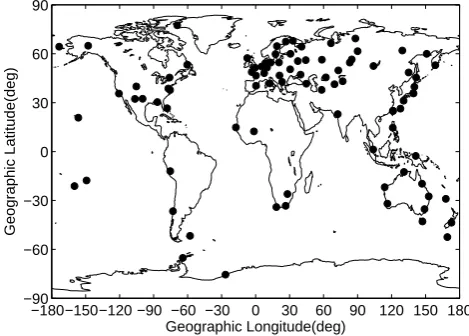
for the accuracy of Eq. (1), it is estimated by Dudeney (1983) that the uncertainty of hmF2 calculated from observed M(3000)F2 is within 4–5%, i.e., about 15–20 km. Thus, the relationship between M(3000)F2 and hmF2 can be taken as true. In the present study, data of M(3000)F2, foF2 and foE used to construct the hmF2 database were downloaded from the Space Physics Interactive Data Resource (SPIDR) web-site http://spidr.ngdc.noaa.gov/. Figure 1 shows the global distribution of the stations used for the present hmF2 global modelling study. In the present work, we used the monthly median data to do the modelling. Therefore, the magnetic activity effects are ignored in the model.

3 Modelling technique description

3.1 Fundamental of EOF analysis method

The modelling technique we used to model hmF2 is mainly based on the empirical orthogonal function (EOF) expan-sion or decomposition of the dataset. EOF analysis method was actually invented by Pearson (1901). This method has been widely and successfully used by meteorologists and oceanographers to analysis the spatial and temporal varia-tions of physical fields since Lorenz (1956) introduced it into meteorology. In the ionospheric field, it was Dvinskikh (1988) who first introduced the EOF analysis into the em-pirical modelling of the ionospheric parameters. His pioneer work was followed by other works (e.g., Singer and Tauben-heim, 1990; Bossy and Rawer, 1990; Singer and Dvinskikh, 1991; Dvinskikh and Naidenova, 1991). It has been shown by many researchers that the EOF analysis is a powerful method in the ionospheric data analysis and empirical mod-elling (e.g., Dvinskikh, 1988; Singer and Dvinskikh, 1991; Dvinskikh and Naidenova, 1991; Daniell et al., 1995; Marsh et al., 2004; Matsuo et al., 2002, 2005; Mao et al., 2005, 2008; Materassia and Mitchell, 2005; Zhao et al., 2005; Zapfe et al., 2006, Liu et al., 2008; Wan et al., 2009, and many more).

EOF analysis involves a mathematical procedure that transforms a dataset into a number of uncorrelated compo-nents called principal compocompo-nents, with any two compocompo-nents orthogonal to each other. Thus, this method sometimes is also named Principal Component Analysis (PCA) or Natural Orthogonal Component (NOC) algorithm. The underlying physical meaning of EOF analysis is that the variation of a physical field variable is mainly controlled by some indepen-dent processes that can be separated. This method decom-poses a dataset into a series of eigen function (or base func-tions) and its associated coefficients, with the base functions orthogonal to each other. As we know, people usually use the Fourier or Spherical Harmonic analysis method to decom-pose a dataset. However, the base function set used in Fourier or Spherical Harmonic analysis is predesigned artificially. In EOF decomposition, the orthogonal base functions are not

−180−150−120 −90 −60 −30 0 30 60 90 120 150 180 −90

−60 −30 0 30 60 90

Geographic Longitude(deg)

Geographic Latitude(deg)

Fig. 1. Global distribution of the stations used for the present mod-elling study.

artificially designed in advance, but are naturally determined by the experimental dataset to be decomposed. Therefore, they possess the inherent characteristics of the original data, and the eigen series will converge very quickly. This makes it possible to use only a few orders of EOF components to represent most of the variance of the original dataset. Hence, the EOF expansion has advantages in data analysis and rep-resentation. In the following, we will briefly describe the fundamentals of the EOF analysis method. For further de-tails, readers are referred to Dvinskikh (1988), Storch and Zwiers (1999) and Xu and Kamide (2004).

LetYij=Y (ti,xj)represent the value of a variable (e.g.,

hmF2) at the spatial point xj(e.g., longitude and latitude)

at timeti,i=1, 2, . . . ,mandj=1, 2, . . . ,n. ThenYm×n is

a matrix ofmrows andn columns. Suppose there are to-tallyrindependent physical processes affecting the variation of the variable, thenY can be decomposed into a series of base functionEk(xj),(j=1,2,...,n)and its associated

co-efficientsAk(ti),(i=1,2,...,m).

Y=

r

X

k=1

Yk(t,x)=

r

X

k=1

Ak(t )EkT(x) (7)

WhereEk= [ek₁,ek₂,...,e_nk]T andAk= [a₁k,ak₂,...,a_mk]T. The superscriptT over a matrix means the transpose of the ma-trix. The base functionsEk(k=1,2,...,r)are uncorrelated, that is, they are orthogonal over space:

EkTEl=

n

X

j=1

e_jkel_j=

1k=l

0k6=l (8)

ek_janda_ikare obtained by minimizing

δ=

m

X

i=1 n

X

j=1

"

Yij− r

X

k=1

a_ike_jk

#2

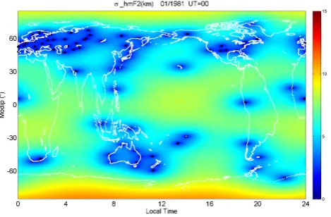
Fig. 2. A sample map of the standard deviation obtained when doing the kriging interpolation.

with respect toe_ik andek_j. In fact, Ek(k=1,2,...,r) is the orthogonal eigenvectors of the symmetric matrixS=YTY, which can be obtained by solving the equation

SEk=λkEk (10)

Whereλk is the eigen value. OnceEk is found, the

associ-ated coefficientAkcan be computed by

Ak=Y Ek (11)

It can be proved that

δ=

m

X

i=1 n

X

j=1

"

Yij− r

X

k=1

a_ikek_j

#2

=

m

X

i=1

λi− r

X

i=1

λi (12)

The percentage variance of the dataset captured by the firstr components is

r

P

i=1

λi

_m P

i=1

λi×100%.

3.2 Data preprocessing and decomposition

Before we can apply the EOF decomposition to the dataset of hmF2, we need to do some data preprocessing work. Since the time periods with available data are different for differ-ent stations, we must normalize the data of each station to the same time period. In this study, we choose the years of 1975–1985 covering both ascending and descending phases of the solar cycle activities as the time period used for global modelling. This time period was chosen because data during this period are available for most of the stations used. To fill the missing data for any station during this period, we pre-processed the data as follows. First, for each single station, with its observational values of M(3000)F2, foF2 and foE as input, M(3000)F2 is converted into hmF2 using Eqs. (1–6). When foE is not available, the value obtained from IRI model is used as input. With the converted hmF2 dataset, single sta-tion model of hmF2 is constructed for each individual stasta-tion using the modelling technique described in Liu et al. (2008).

Then, the missing data (if any), for any chosen station dur-ing the time period of 1975–1985, are filled with the sdur-ingle station model values.

After normalizing all the chosen stations’ data to the time period of 1975–1985 as described above, data at evenly dis-tributed grids (5◦×5◦in a latitudinal range of 85◦S–85◦N and longitudinal range of 0–360◦E) were then obtained by interpolation using Kriging method. To test the validity of the Kriging method in our data preprocessing, the accuracy of Kriging maps is estimated. Figure 2 is a sample but typ-ical map of the standard deviation obtained when doing the Kriging interpolation. In Fig. 2, the black points represent stations whose data is used in interpolation. As can be seen from the figure, the standard deviations of the Kriging maps, at the large areas where observations are sparse, are less than 10 km, which is a very general result in our data preprocess-ing. This means the accuracy of the Kriging maps obtained in our data preprocessing is quite acceptable. The prepared gridded data are the dataset to which the EOF decomposition is going to be applied.

The first step in our modelling is to do the EOF analysis on the gridded dataset prepared as described above. Two lay-ers EOF decomposition are applied. In the first layer, the prepared gridded dataset are decomposed into the EOF base functionsEk(µ, LT), which represent the variation of hmF2

with the modified dip latitude (short:Modip)µand the local time (LT), and the associated EOF coefficients Pk (UT,m),

which represent the variations of hmF2 with the universal time (UT) and seasonal as well as solar cycle variations (de-noted all by the variablem)as the following

hmF2(µ,LT,UT,m)=

N

X

k=1

Ek(µ,LT)·Pk(UT,m) (13)

Here the coordinate (µ, LT) instead of geographical lati-tude/longitude or magnetic latilati-tude/longitude is used since it was found (Rawer, 1963) that features of the ionospheric pa-rameters, in particular those of the F2 layer, are mostly well organized under the coordinate (µ, LT) which is also well confirmed by recent research works (e.g., Azpilicueta et al., 2006) and by our experience when we tried to decompose the dataset using other coordinates such as the geographi-cal latitude/longitude one. This is due to the fact that the ionosphere is controlled by both the orientation of the Earth’s rotation axis and the configuration of the geomagnetic field. Therefore, its variation depends on both the geographical and geomagnetic latitudes, which is embedded in the modipµ defined astgµ=Icos1/2ϕ, whereI is the magnetic incli-nation andϕ the geographical latitude. The ionosphere has also longitudinal variation. In our modelling, the longitudi-nal variation is embedded in the LT (ofEk)and UT (ofPk)

variations since LT=UT+Longitude/15.

In the second layer of EOF decomposition, the coefficients Pk(UT,m) obtained in the first layer EOF analysis are

LT E

1

Modip(

0 )

0 6 12 18 24

−80 −40 0 40 80

0.017 0.018 0.019 0.02 0.021 0.022 0.023

LT E

2

Modip(

0)

0 6 12 18 24

−80 −40 0 40 80

−0.04 −0.03 −0.02 −0.01 0 0.01 0.02 0.03

LT E

3

Modip(

0 )

0 6 12 18 24

−80 −40 0 40 80

−0.04 −0.02 0 0.02 0.04

LT E

4

Modip(

0)

0 6 12 18 24

−80 −40 0 40 80

−0.03 −0.02 −0.01 0 0.01 0.02 0.03 0.04

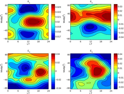
Fig. 3. Distribution of the first four orders of the base functions (E1–E4)obtained with the 1st layer EOF decomposition of hmF2.

representing the variation with the universal time (UT) and the associated coefficientsAj_k(m)representing the seasonal as well as solar cycle variations

Pk(UT,m)= N1

X

j=1

F_kj(UT)·Aj_k(m) (14)

3.3 Modelling the associated EOF coefficientsAj_k(m) The second step in our modelling is to model the EOF coef-ficientsAj_k(m)with the following harmonic functions repre-senting the seasonal (annual and semi-annual) and solar cycle variations. The reason justifying the usage of the following harmonic functions with their amplitudes changing with the solar flux index F10.7to model the coefficientsAjk(m)will be

given in Sect. 4 when we discuss the results obtained by the EOF decompositions.

Aj_k(m)=B_kj₁(m)+B_kj₂(m)+B_kj₃(m) (15) B_kj₁(m)=cj_k1+d_kj₁F10.7(m) (16)

B_kj₂(m)=(c_kj₂+d_kj₂F10.7(m))cos

2π m 12

+(s_kj₂+t_kj₂F10.7(m))sin

2π m

12 (17)

B_kj₃(m)=(c_kj₃+d_kj₃F10.7(m))cos

2π m 6

+(s_kj₃+t_kj₃F10.7(m))sin

2π m

6 (18)

wheremis the month representing the seasonal variation, and F10.7index is a proxy most commonly used to represent the

solar activity levels which was originally called the Coving-ton index (CovingCoving-ton, 1948). It is the solar radio flux density measured at a wavelength of 10.7 cm and expressed in units of 10−22Watts/m2/Hertz. For more details on the proxy so-lar radio flux, please refer to Tobiska (2001) and references therein. With these equations, the coefficientscj_k1,d_kj₁,c_kj₂, d_kj₂,s_kj₂, t_kj₂,c_kj₃, d_kj₃, sj_k3,t_kj₃ are determined by the least-square fitting approaches.

3.4 Model construction

Our model constructions are done in a reversal procedure based on the obtained EOF base functionsEkandF_kjas well

as the coefficientscj_k1,d_kj₁,c_kj₂,d_kj₂,s_kj₂,t_kj₂,cj_k3,d_kj₃,s_kj₃,t_kj₃ obtained. Specifically, to calculate the model value of hmF2 at a given geographical location, one first uses Eqs. (15–18), with the given monthmand the corresponding solar flux in-dexF10.7(m), to calculate the modelled second layer EOF

UT P

1

Year

0 6 12 18 24

1975 1978 1981 1984

1.4 1.5 1.6 1.7 1.8

x 104

UT P

2

Year

0 6 12 18 24

1975 1978 1981 1984

−1500 −1000 −500 0 500 1000

UT P

3

Year

0 6 12 18 24

1975 1978 1981 1984

−1000 −500 0 500 1000

UT P

4

Year

0 6 12 18 24

1975 1978 1981 1984

−1000 −500 0 500

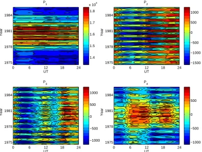
Fig. 4. Distribution of the coefficients (P1–P4)corresponding to the first four orders of base functions (E1–E4)shown in Fig. 3 obtained

with the first layer EOF decomposition of hmF2.

Aj_k and the base functionsF_kj obtained in the second layer EOF decomposition, the modelled first layer EOF coeffi-cientsPkare calculated with Eq. (14). At last, with the

calcu-lated modelledPkand the base functionsEk obtained in the

first layer EOF decomposition, the modelled value of hmF2 is calculated using Eq. (13).

4 Results and discussion

Figure 3 shows the contour plots of the first four orders of the base functionsEk, obtained with the first layer EOF

decom-position of hmF2 dataset, versus the modified dip latitude (µ) and the local time (LT). It can be seen that apparently, the base functionsEk we obtained showed some typical

fea-tures that have been observed in many data. For example, the distribution of the first order of base functionE1

mani-fests mainly a typical phenomenon related to the equatorial ionization anomaly. As is well known, the equatorial ioniza-tion anomaly is a phenomenon characterized by a structure with two crests of ionization (best represented by foF2) at about±17◦dip latitude on each side of the magnetic equator and a trough in between. It is formed as a consequence of the so called “fountain” effect. The influence of this equatorial fountain effects on the F2 peak height hmF2 is that it will

produce a latitudinal distribution of hmF2 with higher value near equatorial and low latitudes but with lower value out-side. This latitudinal distribution structure of hmF2 is exactly what we see in the distribution of the first order of the base functionE1. The second base function E2 mainly reflects

the north-south asymmetry which is closely related to the seasonal change of the solar zenith angle. Because we will see, in Fig. 4, the associated EOF coefficientP2

correspond-ing to this base function shows mainly an annual variation pattern. As for the third base functionE3, the most

remark-able feature to notice is the evening enhancement of hmF2 in the equatorial and low-latitude region. This feature is appar-ently a result of the regeneration/enhancement of the fountain effect during the post-sunset hours due to the evening pre-reversal enhancement (PRE) of the F2 region plasma’s elec-tromagneticE×Bdrift caused by the enhanced zonal elec-tric field near the magnetic equator (Fejer et al., 1995, and references therein). Another feature worth noticing is the en-hancement/abatement ofE3in the north/south auroral zones.

This feature can be explained by combining it with the pat-tern ofP3shown in Fig. 4.P3is positive/negative during the

north winter/summer seasons. Therefore, the contribution of the componentE3×P3is positive/negative during the north

0 4 8 12 16 20 24 −0.5

0 0.5

F1

j

0 4 8 12 16 20 24

−0.5 0 0.5

F2

j

0 4 8 12 16 20 24

−0.5 0 0.5

F3

j

0 4 8 12 16 20 24

−0.5 0 0.5

F4

j

UT

1976 1979 1982 1985

0 2 4 6 8

x 104

A1

j

1976 1979 1982 1985

−4000 −2000 0 2000 4000

A2

j

1976 1979 1982 1985

−2000 0 2000

A3

j

1976 1979 1982 1985

−2000 0 2000

A4

j

Year

j=1 j=2 j=3 j=1 j=2 j=3 Modeled

Fig. 5. Distribution of the base functions (F₁j–F₄j)(left panels) and

their corresponding coefficients (Aj₁–Aj₄) (right panels) obtained with the second layer EOF decomposition of hmF2.

Hemispheres during winter/summer seasons. Therefore, as is demonstrated here, the EOF decomposition analysis method, to some extent, is able to separate the variance of a dataset into components caused by sources due to different physi-cal processes or mechanisms. This demonstrated that EOF analysis is a powerful and advantage method to analyze and organize the ionospheric data.

Figure 4 shows the distribution of the first four orders of the associated coefficientsPkobtained in the first layer EOF

decomposition of hmF2 dataset. They correspond to the first four base functions shown in Fig. 3. It can be seen thatP1

shows a variation pattern with a very strong dependence on the solar cycle activity. It also shows some seasonal varia-tions. The coefficients (P2–P4)corresponding to the other

orders of base functions show most obviously the annual and semi-annual variations, besides, they also show dependence on the solar activity levels.

Figure 5 shows the results obtained in the second layer EOF analysis, that is, the EOF decomposition ofPk. The

left panels are the distributions of the base functionsF_kj ob-tained, the right panels are for the corresponding associated coefficientsAj_k. The different curves are for the first three components (j=1, 2, 3). ForAj_k, the results modelled with Eqs. (15–18) are also plotted (thin green curves overlaying on each corresponding decomposed ones). As we can see from the right panels, the second layer EOF coefficientsAj_k mainly contains the annual and semiannual variation com-ponents and their amplitudes also change with the solar cy-cle activity levels. This justifies the modelling of the coeffi-cientsAj_k with the harmonic functions representing the sea-sonal (annual and semi-annual) variations as well as their

so-100 150 200 250 300 350 400 450 500

100 200 300 400 500

Year= 1976 R= 0.9392

Model hmF2(km)

200 250 300 350 400 450 500 550 600

200 300 400 500 600

Year= 1981 R= 0.94538

Observed hmF2(km)

Model hmF2(km)

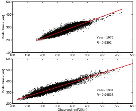
Fig. 6. Scatter plots of model value versus observational data of

hmF2.

lar cycle activity dependence represented by the F10.7index

as expressed by Eqs. (15–18). As can be seen from the fig-ure, the modelled coefficientsAj_kreplicated the original ones very well.

250

LY164

IRI EOF_hmF2 EOF_M3000F2 OBS

250

YA462

250

WK545

250 350

YG431

250

MA720

hmF2(km)

250 350

450 _SI301

250

350 HU91K

250

MU43K

250

HO54K

Jan. Feb. Mar. Apr. May Jun. Jul. Aug. Sep. Oct. Nov. Dec.

200

300 PSJ5J

300

LY164

IRI EOF_hmF2 EOF_M3000F2 OBS

250

350 YA462

250

350 WK545

250

350 YG431

250

350 MA720

hmF2(km)

300 400 500

SI301

300

400 HU91K

250 350

MU43K

250

350 HO54K

Jan. Feb. Mar. Apr. May Jun. Jul. Aug. Sep. Oct. Nov. Dec.

250

350 PSJ5J

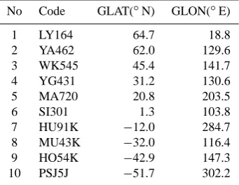
Fig. 7. Sample plots of model values and observational data of hmF2 for the years of (a) 1965 and (b) 1970. From top to bottom panels, stations are ordered from north high, middle and low latitudes to the south low, middle and high latitudes.

Table 1. Geographical coordinates of the stations labeled in Fig. 7a–b.

No Code GLAT(◦N) GLON(◦E)

1 LY164 64.7 18.8

2 YA462 62.0 129.6

3 WK545 45.4 141.7

4 YG431 31.2 130.6

5 MA720 20.8 203.5

6 SI301 1.3 103.8

7 HU91K −12.0 284.7

8 MU43K −32.0 116.4

9 HO54K −42.9 147.3

10 PSJ5J −51.7 302.2

IRI model results, whereas the blue points are the observa-tional data. As an addiobserva-tional comparison, results provided by the EOF-based M(3000)F2 model (Liu et al., 2008) are also shown (thin red curves). They are obtained by converting the modelled M(3000)F2 to hmF2 using Eqs. (1–6). As can be seen from these plots, the EOF model results (both of hmF2

and M(3000)F2) in general reproduced quite well the vari-ation behaviour of the observvari-ational data. Compared with the results given by the IRI model, the EOF model results compare obviously better than the IRI model results with the observational data. As for the EOF model results, it can be seen from Fig. 7a–b that, in general, the results based on the M(3000)F2 model are very similar to those provided by the hmF2 model. However, a careful inspection of the details of the plots indicates that the hmF2 model results are somewhat improved over the M(3000)F2 model results.

To estimate the accuracy of the model, we made a statis-tical analysis on differences between the model values and the observational data by calculating the root-mean-squared-error (RMSE) of the model:

RMSE=

v u u t

1 Np

Np

X

i=1

(hmF2model−hmF2obs)2 (19)

WhereNpis the total number of the data points.

and 14.3 km for the years 1965 and 1970, respectively. As a comparison, the RMSEs for the IRI model results are 18.9 km and 22.6 km for the year 1965 and 1970, respec-tively. Therefore, in general, our constructed global model of hmF2 based on the EOF decomposition has a higher ac-curacy than the model currently used in IRI. The acac-curacy of the EOF-based hmF2 model is also slightly higher than that of the global EOF-based M(3000)F2 model (in terms of the converted hmF2).

5 Summary and conclusion

In the present study, an attempt was made to construct the global model of the ionospheric F2 peak height parameter hmF2 based on the EOF decomposition of the dataset and the modelling of the associated EOF coefficients with harmonic functions representing annual and semi-annual seasonal vari-ations. Solar cycle dependence is also taken into account in the model by including the changes of the harmonic ampli-tudes with the solar irradiance flux index F10.7. Comparisons

between the model predictions and the observational data are in agreement. Statistical analysis on the differences between model values and observational data showed the constructed model of hmF2 based on the EOF expansion agrees better with the observational data than the model currently used in IRI. The accuracy of the hmF2 model developed in this study is slightly higher than that of the global EOF-based M(3000)F2 model (in terms of converted hmF2) previously developed by our team (Liu et al., 2008). From the point of view of practical application, the hmF2 model is more prefer-able than the M(3000)F2 global model, since in many appli-cations it is the parameter hmF2, rather than M(3000)F2, that is really required. It is also due to the fact that the conver-sion from M(3000)F2 to hmF2 involves the foF2/foE ratio. It would be much more convenient to obtain hmF2 directly from a reliable hmF2 global model than converting to hmF2 from an M(3000)F2 model.

Acknowledgements. This research was supported by the National

Natural Science Foundation of China (40890164, 40774092), the National Important Basic Research Project (2006CB806306) and the China Meteorological Administration Grant (GYHY20070613). The M(3000)F2, foF2, foE and F10.7index data used for the

mod-elling study were downloaded from the SPIDR web site http://spidr. ngdc.noaa.gov/. The author Man-Lian Zhang gratefully acknowl-edges the support of K. C. Wong Education Foundation, Hong Kong. We would also like to thank the two referees for their sug-gestions to improve the manuscript of this paper.

Topical Editor M. Pinnock thanks Shunrong Zhang and another anonymous referee for their help in evaluating this paper.

References

Adeniyi, J. O., Bilitza, D., Radicella, S. M., and Willoughby, A. A.: Equatorial F2-peak parameters in the IRI model, Adv. Space.

Res., 31(3), 507–512, doi:10.1016/S0273-1177(03)00039-5, 2003.

Azpilicueta, F., Brunini, C., and Radicella, S. M.: Global iono-spheric maps from GPS observations using modip latitude, Adv. Space Res., 38(11), 2324–2331, doi:10.1016/jasr.2005.07.069, 2006

Bilitza, D.: International Reference Ionosphere 1990, Rep. NSSDC/WDC-R&S 90-22, World Data for Rockets and Satell., Nat. Space Sci. Data Cent., Greenbelt, Md., 1990.

Bilitza, D.: International Reference Ionosphere 2000, Radio Sci., 36(2), 261–275, doi:10.1029/2000RS002432, 2001.

Bilitza, D., Sheikh, N. M., and Eyfrig, R.: A global model for the height of the F2-peak using M3000 values from the CCIR nu-merical map, Telecommun. J., 46, 549–553, 1979.

Bossy, L. and Rawer, K.: Discussion of a new method for map-ping ionospheric characteristics, Adv. Space Res., 10(11), 65–74, doi:10.1016/0273-1177(90)90307-L, 1990.

Bradley, P. A. and Dudeney, J. R.: A simple model of the vertical distribution of electron concentration in the ionosphere, J. At-mos. Terr. Phys., 35, 2131–2146, 1973.

CCIR: Comite Consultatif International des Radiocommunications, Reports 340, 340-2 and later supplements, Geneva, 1967. Covington, A. E.: Solar noise observations on 10.7 centimeters,

Proc. IRE, 36, 454–457, 1948.

Daniell, R. E., Brown Jr., L. D., Anderson, D. N., Fox, M. W., Doherty, P. H., Decker, D. T., Sojka, J. J., and Schunk, R. W.: Parameterized ionospheric model: A global ionospheric param-eterization based on first principles models, Radio Sci., 30(5), 1499–1510, doi:10.1029/95RS01826, 1995.

Dvinskikh, N. I.: Expansion of ionospheric characteristics fields in empirical orthogonal functions, Adv. Space Res., 8(4), 179–187, doi:10.1016/0273-1177(88)90238-4, 1988.

Dvinskikh, N. I. and Naidenova, N. Ya.: An adaptable regional empirical ionospheric model, Adv. Space Res., 11(10), 7–10, doi:10.1016/0273-1177(91)90312-8, 1991.

Dudeney, J. R.: The accuracy of simple methods for determining the height of the maximum electron contration of the F2-layer from scaled ionospheric characteristics, J. Atmos. Terr. Phys., 45(8– 9), 629–640, 1983.

Eyfrig, R.: Eine Bemerkung zur Bradley-Dudeney’schen Modell Ionosphaere, Kleinheubacher Berichte, 17, 199–202, 1973. Fejer, B. G., de Paula, E. R., Heelis, R. A., and Hanson, W. B.:

Global equatorial ionospheric vertical plasma drifts measured by the AE-E satellite, J. Geophys. Res., 100(4), 5769–5776, 1995. Gulyaeva, T. L., Bardley, P. A., Stanislawskw, I., and Juchnikowski,

G.: Towards a new reference model of hmF2 for IRI, Adv. Space. Res., 42, 666–672, 2008.

Leitinger, R., Zhang, M.-L., and Radicella S. M.: An improved bottomside for the ionospheric electron density model NeQuick, Ann. Geophys., 48(3), 525–534, 2005.

Liu, C., Zhang, M.-L., Wan, W., Liu, L., and Ning, B.: Modelling M(3000)F2 based on empirical orthogonal function analysis method, Radio Sci., 43, RS1003, doi:10.1029/2007RS003694, 2008.

Lorenz, E. N.: Empirical orthogonal functions and statistical weather prediction, Technical report, Statistical Forecast Project Report 1, Dept. of Meteor., MIT, 48pp, 1956.

Mao, T., Wan, W., Yue, X., Sun, L., Zhao, B., and Guo, J.: An em-pirical orthogonal function model of total electron content over China, Radio Sci., 43, RS2009, doi:10.1029/2007RS003629, 2008.

Marsh, D. R., Solomon, S. C., and Reynolds, A. E.: Empirical model of nitric oxide in the lower thermosphere, J. Geophys. Res., 109, A07301, doi:10.1029/2003JA010199, 2004.

Materassia, M. and Mitchell, C. N.: A simulation study into constructing of the sample space for ionospheric imaging, J. Atmos. Sol. Terr. Phys., 67, 1085–1091, doi:10.1016/j.jastp.2005.02.019, 2005.

Matsuo, T., Richmond, A. D., and Nychka, D. W.: Modes of high-latitude electric field variability derived from DE-2 mea-surements: Empirical Orthogonal Function (EOF) analysis, Geophys. Res. Lett., 29(7), 1107, doi:10.1029/2001GL014077, 2002.

Matsuo, T., Richmond, A. D., and Lu, G.: Optimal interpolation analysis of high-latitude ionospheric electrodynamics using em-pirical orthogonal functions: Estimation of dominant modes of variability and temporal scales of large-scale electric fields, J. Geophys. Res., 110, A06301, doi:10.1029/2004JA010531, 2005. Obrou, O. K., Bilitza, D., Adeniyi, J. O., and Radicella, S. M.: Equatorial F2-layer peak height and correlation with vertical ion drift and M(3000)F2, Adv. Space Res., 31(3), 513–520, doi:10.1016/S0273-1177(03)00024-3, 2003.

Oyeyemi, E. O., Mckinnell, L. A., and Poole, A. W. V.: Neu-ral network-based prediction techniques for global modelling of M(3000)F2 ionospheric parameter, Adv. Space Res., 39(5), 643– 650, doi:10.1016/j.asr.2006.09.038, 2007.

Pearson, K.: On lines and planes of closest fit to systems of points in space, Phil. Mag., 6, 559–572, 1901.

Radicella, S. M. and Leitinger, R.: The evolution of the DGR approach to model electron density profiles, Adv. Space. Res., 27(1), 35–40, doi:10.1016/S0273-1177(00)00138-1, 2001. Rawer, K.: Meteorological and Astronomical Influences on Radio

Wave Propagation, ed. B. Landmark, Pergamon Press., Oxford, pp. 221–250, 1963.

Rawer, K., Ramakrishnan, S., and Bilitza, D.: International Refer-ence Ionosphere, International Union of Radio SciRefer-ence, Special Report, Brussels, Belgium, 1978.

Shimazaki, T.: World-wode daily variations in the height of the maximum electron of the ionospheric F2-layer, J. Radio Res. Lab. 2(7), 85–97, 1955.

Singer, W. and Dvinskikh, N. I.: Comparison of empirical models of ionospheric characteristics developed by means of different map-ping methods, Adv. Space Res., 11(10), 3–6, doi:10.1016/0273-1177(91)90311-7, 1991.

Singer, W. and Taubenheim, J.: Application of the expansion into empirical orthogonal functions to ionospheric character-istics, Adv. Space Res., 10(11), 59–64, doi:10.1016/0273-1177(90)90306-K, 1990.

Storch, H. V. and Zwiers, F. W.: Statistical Analysis in Climate Research, Cambridge University Press, 1999.

Tobiska, W. K.: Validating the solar EUV proxy, E10.7, J. Geophys.

Res., 106(A12), 29969–29978, 2001.

Wan, W., Ding, F., Zhang, M.-L., Liu, L., and Ning, B.: Modelling the Global Ionospheric TEC with Statistical Eigen Mode Analy-sis, Adv. Space Res., in review, 2009.

Wright, J. W. and Mcduffie, R. E.: The relation of hmaxF2 to M(3000)F2 and hpF2, J. Radio Res. Lab (Tokyo), 7(32), 498– 520, 1960.

Xu, W.-Y. and Kamide, Y.: Decomposition of daily geomagnetic variations by using method of natural orthogonal component, J. Geophys. Res., 109, A05218, doi:10.1029/2003JA010216, 2004. Zapfe, B. D., Materassi, M., Mitchell, C. N., and Spalla, P.: Imaging of the equatorial ionospheric anomaly over South America – A simulation study of total electron content, J. Atmos. Sol. Terr. Phys., 68, 1819–1833, doi:10.1016/j.jastp.2006.05.025, 2006. Zhang, M. L., Shi, J. K., Wang, X., Wu, S. Z., and Zhang,

S. R.: Comparative study of ionospheric characteristic pa-rameters obtained by DPS-4 digisonde with IRI2000 for low latitude station in China, Adv. Space Res., 33(6), 869–873, doi:10.1016/j.asr.2003.07.013, 2004.

Zhang, M. L., Shi, J. K., Wang, X., Shang, S. P., and Wu, S. Z.: Ionospheric behavior of the F2 peak parameters foF2 and

hmF2 at Hainan and comparisons with IRI model predictions,

Adv. Space Res., 39(5), 661–667, doi:10.1016/j.asr.2006.03.047, 2007.