Compression for Fixed-Width Memories
Ori Rottenstreich, Amit Berman, Yuval Cassuto and Isaac Keslassy
Technion
{
or@tx, bermanam@tx, ycassuto@ee, isaac@ee
}
.technion.ac.il
Abstract—To enable direct access to a memory word based on its index, memories make use of fixed-width arrays, in which a fixed number of bits is allocated for the representation of each data entry. In this paper we consider the problem of encoding data entries of two fields, drawn independently according to known and generally different distributions. Our goal is to find two prefix codes for the two fields, that jointly maximize the probability that the total length of an encoded data entry is within a fixed given width. We study this probability and develop upper and lower bounds. We also show how to find an optimal code for the second field given a fixed code for the first field.
I. INTRODUCTION
Fixed-width memories are particularly appealing for net-working applications. They enable a direct access to a memory word regardless of its index. This property is mandatory, for in-stance, in hash-based implementations of forwarding tables [1]. We consider the encoding of data entries with d= 2fields, drawn independently according to two known distributions, within a bound of L bits corresponding to the fixed width of a memory word. We would like to find two prefix codes for the two fields, so as to maximize the probability that the total length of the two codewords in the encoding of a data entry is at most L bits. Unfortunately, we will show that popular techniques for data compression such as Huffman coding [2] are not necessarily optimal for this metric.
Consider for instance a data entry with two fields, such that the value of the first field is among four possible elements {a, b, c, d}, and the second is one of the two elements{x, y}. As summarized in Table I.(A)-(B), these possible values appear with different probabilities, and the values of the two fields are drawn independently. For instance, the first field has the value
aw.p. (with probability)0.4,andbw.p.0.3. We encode the two fields using two prefix codes σ1, σ2. As shown in Table I.(C),
the selection of these codes determines the obtained width for the 4·2 = 8possible data entries. Here, the minimal obtained width of an encoded data entry is 2 bits, and the maximal width is 4 bits. If the allowed fixed-width is L= 3, only four of the data entries can be encoded successfully (presented with √), while four others will have to be stored in a different memory hierarchy and will result in a slower access time. Accordingly, we say that the obtained success probability for this encoding scheme CD = (σ1, σ2) is the sum of probabilities for the
successfully-encoded entries, i.e.
Psuccess(L= 3, CD) = 0.24 + 0.16 + 0.09 + 0.06 = 0.55.
Recently, an encoding scheme that minimizes the maximal encoding width of a given set of data entries was suggested
(A) First field with codeσ1 Element Prob. codeword
a 0.4 0
b 0.3 110
c 0.15 10
d 0.15 111
(B) Second field with codeσ2 Element Prob. codeword
x 0.6 0
y 0.4 1
(C) Possible entries encoded by the encoding schemeCD= (σ1, σ2)
Entry Prob. Encoding Width (ℓ) ℓ≤(L= 3)
(a,x) 0.24 0 0 2 √
(a,y) 0.16 0 1 2 √
(b,x) 0.18 110 0 4
-(b,y) 0.12 110 1 4
-(c,x) 0.09 10 0 3 √
(c,y) 0.06 10 1 3 √
(d,x) 0.09 111 0 4
-(d,y) 0.06 111 1 4
-TABLE I
EXAMPLE OFENCODINGSCHEME. (A)AND(B)ILLUSTRATE THE ENTRY DISTRIBUTION OF TWO FIELDS,AND THEIR RESPECTIVE CODESσ1ANDσ2.
(C)SHOWS THE RESULTING ENCODING SCHEMECD= (σ1, σ2),USING
THE CONCATENATION OF THE CORRESPONDING TWO CODEWORDS FOR THE TWO FIELDS. (SPACES ARE PRESENTED FOR SIMPLICITY AND DO NOT EXIST IN PRACTICE.) IN THIS EXAMPLE,FOUR POSSIBLE DATA ENTRIES
ARE ENCODED SUCCESSFULLY WITHINL= 3BITS,AND
Psuccess(L= 3, CD) = 0.24 + 0.16 + 0.09 + 0.06 = 0.55.
in [3]. Unfortunately, the fixed width of a memory array is typically predetermined by its manufacturer and cannot be changed dynamically by the user. Furthermore, the worst-case approach of [3] may be too stringent. Therefore, the new probabilistic model we consider here of maximizing the success probability for a fixed L is a more realistic one. We note that the occasional failures to meet the fixed width can easily be accommodated in practice by sending the data entry to a slower (e.g. DRAM) memory instead of the main (e.g. SRAM) memory. A high success probability will guarantee good access time on average.
II. MODEL ANDPROBLEMFORMULATION
A. Terminology
We start by describing the terminology we use throughout this study. For short, we refer to a data entry simply as an entry.
Definition 1 (Entry Distribution). An entry distribution D = ((S1, P1),(S2, P2)) =
(
({s1,1, . . . , s1,n1}, (p1,1, . . . , p1,n1)),
({s2,1, . . . , s2,n2}, (p2,1, . . . , p2,n2))
)
is characterized by two (ordered) sets of elements with their corresponding vectors of positive appearance probabilities. An entry (a1, a2) has two
fields drawn randomly and independently according to the dis-tributionDs.t.Pr (a1=s1,i) =p1,iandPr (a2=s2,i) =p2,i
with p1,i, p2,i > 0. The numbers of possible elements in the
first and second field of an entry aren1=|S1|and n2=|S2|,
respectively.
Example 1. The entry distribution of the two fields illustrated in Table I, can be summarized asD= ((S1, P1),(S2, P2)) =
(
({a, b, c, d},(0.4,0.3,0.15,0.15)),({x, y},(0.6,0.4))
)
.
Definition 2(Prefix Code). For a set of elementsS, a codeσ
is an injective mappingσ:S→B, whereB is a set of binary codewords of size |B|=|S|. A code is called aprefix code if no binary codeword inB is a prefix (start) of any other binary codeword in B.
Definition 3(Encoding Scheme). Anencoding schemeCD of
an entry distribution D is a pair of two prefix codes CD = (σ1, σ2). That is, eachσj is a prefix code of the set of elements Sj in the first or the second field.
Our main motivation for using prefix codes is the simplicity they enable in the representation of encoded entries in the mem-ory. For each encoded entry, we simply keep the concatenation of the two codewords for each of its fields. It is easy to verify that the properties of the prefix codes (and indeed only of the first of them) guarantee that different entries yield different (concatenated) encodings.
For a binary string x, let ℓ(x) denote the length in bits of
x. With an encoding scheme CD = (σ1, σ2), we say that the
encoding width of an entry(a1, a2)is ℓ(σ1(a1)) +ℓ(σ2(a2)).
Next, we define the encoding width bound. With this bound, we can distinguish between different encoding schemes based on their obtained encoding widths for the possible entries.
Definition 4 (Encoding Width Bound). Given an encoding scheme CD = (σ1, σ2) and an encoding width bound of L
bits, we say that an entry(a1, a2)is encoded successfully if its
encoding width is not larger than the encoding width bound, i.e.
(
ℓ(σ1(a1)) +ℓ(σ2(a2))
)
≤L.
B. Optimal Encoding Scheme for an Entry Distribution
We would like now to define the main problem that we address in this study. Given an entry distribution D = ((S1, P1),(S2, P2))and an encoding width boundL, we would
like to find an encoding schemeCD= (σ1, σ2)that maximizes
the probability that an encoding of an arbitrary entry would be successful. For the scheme CD, we denote this probability by Psuccess(L, CD).
We remind that we limit each of the two codes σ1, σ2
to be prefix. Therefore, the lengths of the binary codewords in each of the codes must satisfy Kraft’s inequality, i.e.
∑
a∈Sj2
−ℓ(σj(a))≤1(forj∈[1,2]). In addition, these lengths are clearly positive integers.
We can now express the problem as the following optimiza-tion problem. Here,I(·)is the indicator function that takes the value of 1 if the condition that it receives as a parameter is satisfied, and 0 otherwise.
max Psuccess = n1
∑
i=1
n2
∑
j=1
p1,i·p2,j·I
(
ℓ(σ1(s1,i)) +ℓ(σ2(s2,j))≤L
)
s.t. ∑
a∈Sj
2−ℓ(σj(a)) ≤1,∀j∈[1,2] (1a)
ℓ(σj(a))>0∀j∈[1,2],∀a∈Sj (1b)
ℓ(σj(a))∈Z∀j ∈[1,2],∀a∈Sj. (1c)
Assuming an entry distribution D = ((S1, P1),(S2, P2)),
we denote byOP T(L)the optimal success probability, i.e. the maximal possible value of Psuccess that can be obtained by any encoding scheme CD as a function of a positive integer encoding width boundL. Formally,
OP T(L) = max CD=(σ1,σ2)
Psuccess(L, CD). (2)
We say that an encoding schemeCD isoptimalfor a given Liff it satisfiesPsuccess(L, CD) =OP T(L).
III. OBSERVATIONS
In this section, we suggest some basic observations regarding our problem. For the sake of simplicity, throughout the paper we assume that each field can hold the same number of n= n1 = n2 = 2W possible elements. We also assume that for
j∈[1,2], the elementsSj={sj,1, . . . , sj,nj}are ordered in a non-increasing order of their probabilities such thatpj,i1 ≥pj,i2
ifi1< i2.
For any entry distribution D = ((S1, P1),(S2, P2)), the
optimal success probability OP T(L) ∈ [0,1] is clearly a non-decreasing function of the parameterL. Let the encoding scheme CF = (σF1, σ2F) be composed of two fixed-length
codes, such that both encode each of the2W elements ofS1, S2
by a codeword ofW bits.
Property 1. The optimal success probability satisfies (i)ForL≥2W OP T(L) = 1,and for L <2W
OP T(L)≤1−
( 2W
∑
i=2W−1
p1,i
)
·
( 2W
∑
i=2W−1
p2,i
)
.
Proof: (i) OP T(L) = 1 for L ≥ 2W can be proved by the encoding schemeCF, in which the obtained encoding width of any entry is clearly W +W = 2W. Thus 1 = Psuccess(L, CF)≤OP T(L). In addition, by Kraft’s inequality, in any encoding schemeCD, at least(2W−1+1)elements inS1
and at least(2W−1+ 1)inS
2are encoded with at leastW bits.
In the best case, these longer codewords will be assigned to the lowest-probability elements. IfL <2W an entry composed of two such elements is not encoded successfully. This gives the second part of (i).
(ii) If L = 2, let’s show that there is at most a single entry that can be encoded successfully. A legally encoded entry must be an entry composed of a pair of elements (one from
S1 and another from S2), where each element is encoded
within a single bit by σ1 and σ2. By Kraft’s inequality, in
both codes, there must be at most one such element when
W ≥ 2. The maximal success probability is obtained in an encoding scheme CD that encodes in a single bit the most common elements in both sets s1,1 ∈ S1, s2,1 ∈ S2. Then,
OP T(2) =Psuccess(L, CD) =p1,1·p2,1.
The encoding schemeCF satisfiesP
success(L, CF) = 0 for L <2W. Then, based on the proof of the last property we can immediately observe the following.
Property 2. For W ≥2, the encoding scheme CF composed
of two fixed-length codes with codewords ofW bits is optimal forL≥2W,and is not optimal forL∈[2,2W−1].
The next lemma suggests the intuitive result that we should prefer to use shorter codewords for elements that appear more often. It is also interesting because it reduces the search space for the optimal code.
Definition 5(Monotone Coding). An encoding scheme CD= (σ1, σ2)of entry distributionD= ((S1, P1),(S2, P2))is called
monotoneif for j∈[1,2],i1 < i2 implies thatℓ(σj(sj,i1))≤
ℓ(σj(sj,i2)).
Lemma 1. For any entry distributionD= ((S1, P1),(S2, P2))
and any L ≥ 1, there exists a monotone optimal encoding scheme.
Proof: We show how to build an optimal monotone encoding scheme based on any optimal encoding scheme
CD= (σ1, σ2). Consider two arbitrary indicesi1, i2that satisfy
i1 < i2. Then necessarily p1,i1 ≥ p1,i2. If ℓ(σ1(s1,i1)) >
ℓ(σ1(s1,i2)), we can replaceσ1by a new code obtained by
per-muting the two codewords ofs1,i1, s1,i2. With this change, an
entry(a1=s1,i1, a2)is encoded successfully after the change
only if the entry(a1 =s1,i2, a2) was encoded successfully in
CD(and vice versa). Likewise, if before the change, the first of them was encoded successfully then also the second. Then, we can deduce that such a change cannot decrease Psuccess and the result follows. We do the same forσ2 and conclude.
We next prove that the success probability of encodings with short average code length can be bounded from below. This will be shown by a refinement of the Markov inequality. For
D = ((S1, P1),(S2, P2)), CD = (σ1, σ2) let E(CD) =
∑n1
i=1
∑n2
j=1p1,i·p2,j·
(
ℓ(σ1(s1,i)) +ℓ(σ2(s2,j))
)
=
∑n1
i=1p1,i·ℓ(σ1(s1,i)) +
∑n2
j=1p2,j·ℓ(σ2(s2,j)).
Property 3. The encoding scheme CD = (σ1, σ2) for D =
((S1, P1),(S2, P2))with an average encoding width ofE(CD)
satisfies Psuccess(L, CD)≥ L+1L−−E1(CD) = 1−E(CLD−)1−2.
Proof:An unsuccessfully encoded entry has a width of at least(L+1)bits while the width of any encoded entry is at least 2 bits. We then have thatE(CD)≥
(
(1−Psuccess(L, CD))·
(L+ 1) +Psuccess(L, CD)·2
)
. The result then follows. We now consider a special option for the encoding scheme. The schemeCH
D = (σ1, σ2)is constructed s.t.σ1is a Huffman
code ofS1(with its probability vectorP1) andσ2is a Huffman
code ofS2[2]. A Huffman code minimizes the expected length
of a codeword. Unfortunately, as shown in the next example, an encoding schemeCH
D composed of two Huffman codes (for S1, S2) is not necessarily optimal.
Example 2. As illustrated in Fig. 1 and Fig. 2 , letn1=n2=
4 = 2W for W = 2. Likewise, letD = ((S
1, P1),(S2, P2)) =
(
({s1,1, s1,2, s1,3, s1,4}, (p1,1 = 0.9, p1,2 = 0.06, p1,3 =
0.03, p1,4= 0.01)), ({s2,1, s2,2, s2,3, s2,4}, (p2,1= 0.5, p2,2=
0.2, p2,3 = 0.15, p2,4 = 0.15))
)
and let the encoding width bound beL= 3.
As shown in Fig. 1, let σ1, σ2 be Huffman codes of S1, S2
and let CH
D = (σ1, σ2) be the encoding scheme composed
of these codes. Since (pj,3 +pj,4) < pj,1 and pj,2 < pj,1
for j ∈ [1,2] then necessarily σj satisfies ℓ(σj(sj,1)) =
1, ℓ(σj(sj,2)) = 2, ℓ(σj(sj,3)) = 3, ℓ(σj(sj,4)) = 3. To
calculatePsuccess(L, CDH), we can see that there are 3 entries
that are encoded successfully within L = 3 bits: (s1,1, s2,1),
(s1,1, s2,2),(s1,2, s2,1). Accordingly, Psuccess(L, CDH) = 0.9· 0.5 + 0.9·0.2 + 0.06·0.5 = 0.66.
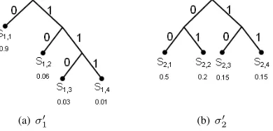
A second encoding scheme CD = (σ′1, σ′2) is presented in
Fig. 2. This scheme satisfies ℓ(σ1′(s1,1)) = 1, ℓ(σ1′(s1,2)) =
2, ℓ(σ′1(s1,3)) = 3, ℓ(σ1′(s1,4)) = 3 (as in CDH) while ℓ(σ′2(s2,1)) = ℓ(σ2′(s2,2)) = ℓ(σ2′(s2,3)) = ℓ(σ2′(s2,4)) =
2. Here, 4 entries can be encoded successfully: (s1,1, s2,1),
(s1,1, s2,2), (s1,1, s2,3), (s1,1, s2,4) and Psuccess(L, CD) = 0.9·0.5 + 0.9·0.2 + 0.9·0.15 + 0.9·0.15 = 0.9 > 0.66 = Psuccess(L, CDH).
Although the encoding scheme CH
D is not necessar-ily optimal, by Property 3 it satisfies Psuccess(L, CDH) ≥
L+1−E(CHD)
L−1 = 1−
E(CDH)−2
L−1 where E(C
H
D) is the minimal possible average encoding width among all possible encoding schemes.
IV. BOUNDS ON THEOPTIMALSUCCESSPROBABILITY
In this section we present upper and lower bounds on the optimal success probability for a given entry distributionD= ((S1, P1),(S2, P2))and an encoding width bound of Lbits.
(a)σ1 (b)σ2
Fig. 1. Illustration of the encoding schemeCDH = (σ1, σ2)composed of twoHuffmancodesσ1ofS1={s1,1, s1,2, s1,3, s1,4}(presented in (a) with probabilities (0.9,0.06,0.03,0.01)) andσ2 ofS2={s2,1, s2,2, s2,3, s2,4}(in (b) with probabilities (0.5,0.2,0.15,0.15)). For instance,σ1(s1,1) = 0 and σ2(s2,3) = 110.CDHsatisfiesPsuccess(L= 3, CHD) = 0.66.
(a)σ1′ (b)σ′2
Fig. 2. Illustration of a second encoding schemeCD = (σ1′, σ2′)with an improved success probabilityPsuccess(L= 3, CD) = 0.9.
schemes. In each scheme, we divide the L bits between the two fields into ℓ and (L−ℓ) bits. Then, in all successfully encoded entries, the first field is encoded in ℓ bits while the second in (L−ℓ) bits. We consider values of ℓ such that
ℓ,(L−ℓ) are both positive and are not greater than W, i.e.
ℓ∈[a, b] = [max(1, L−W),min(L−1, W)]. The lower bound is presented in the following theorem.
Theorem 2. The optimal success probability satisfies
OP T(L)≥ max ℓ∈[a,b]
((2ℓ−1
∑
i=1
p1,i
)
·
(2L−ℓ−1
∑
i=1
p2,i
))
. (3)
Proof: For a given ℓ, we consider a code σ1 of S1 in
which the first n1,1= 2ℓ−1elements (with larger probability)
are encoded within ℓ bits while the last n1,2 = n −n1,1
elements are encoded in (ℓ+⌈log2(n1,2)⌉) bits. We can see
thatn1,1·2−ℓ+n1,2·2−(ℓ+⌈log2(n1,2)⌉)= (2ℓ−1)·2−ℓ+n
1,2·
2−(ℓ+⌈log2(n1,2)⌉)≤1−2−ℓ+ 2−ℓ= 1, and as a consequence
such a prefix code exists. We similarly encode all the first
n2,1= 2(L−ℓ)−1 elements ofS2 in(L−ℓ)bits and the other
n2,2=n−n2,1elements in((L−ℓ)+⌈log2(n2,2)⌉)bits. Then,
any entry composed of two elements from the first n1,1, n2,1
elements in S1, S2 has an encoding width ofℓ+ (L−ℓ) =L
bits and as a result is encoded successfully.
Next, we discuss an upper bound onOP T(L). By Lemma 1 it is enough to show this only for monotone encoding schemes. We use the notationsℓ1,i=ℓ(σ1(s1,i)),ℓ2,i =ℓ(σ2(s2,i)) for i∈[1, n] and haveℓ1,i≤ℓ1,j, ℓ2,i≤ℓ2,j if i < j.
By Kraft’s inequality, for ℓ ∈ [1, W −1], at least one of the first 2ℓ elements in S1, S2 is encoded with at least ℓ+ 1
bits, because there are additional elements that still need to be encoded. Based on this observation and the assumed order of the codeword lengths, we can deduce lower bounds on these lengths. For instance, if W ≥ 3, we cannot encode the first two elements in a single bit, and one of the first four elements must be encoded with at least three bits. Thus
ℓj,2≥2, ℓj,4≥3 for j ∈[1,2] since we consider a monotone
encoding scheme and accordingly ℓj,i ≥ 2 for i ∈ [2,3] and ℓj,i ≥ 3 for i ∈ [4,8]. More generally, we can show that ℓj,i ≥
⌈
log2(i+I(i <2W))⌉ for i ∈ [1, n = 2W]. Based on this lower bound, we denote byf(ℓ) forℓ∈[1, W] the index of the first element that must be encoded in at leastℓ bits, i.e.
f(ℓ) = mini∈[1,n]
( ⌈
log2(i+I(i <2W))⌉≥ℓ
)
= 2ℓ−1. Let
[a, b] = [max(1, L+ 1−W),min(L, W)]. We are now ready to present the bound.
Theorem 3. The optimal success probability satisfies
OP T(L)≤ min ℓ∈[a,b]
(
1−
( 2W
∑
i=2ℓ−1
p1,i
)
·
( 2W
∑
i=2L−ℓ
p2,i
))
.
Proof:Forℓ∈[1, L]that satisfiesℓ,(L+ 1−ℓ)≤W, the encoding width of an entry composed of two elements encoded in at leastℓand(L+1−ℓ)bits, respectively, is at leastℓ+(L+ 1−ℓ) =L+ 1 bits. Therefore, any such entry is not encoded successfully and cannot contribute to the success probability of a monotone encoding scheme. By Lemma 1, we can generalize the result to any encoding scheme, and the result follows.
V. OPTIMALCONDITIONALCODE OF THESECONDFIELD
The ultimate goal of this work is an algorithm that finds for a general value ofL, an optimal two-field encoding scheme that jointly maximizes the success probability. An intermediate step toward this goal is an algorithm that finds the optimal encoding of one field, conditioned on the encoding of the other field. Such an algorithm is the topic of this section. This algorithm has a value in its own right (e.g., when one field encoding is set by external constraints), and also as a likely component in a future optimal two-field algorithm.
Finding an optimal encoding scheme whenL≥2W is easy. By Property 2, the encoding scheme CF is an example for such a scheme. In this section we consider the case where
L ≤ (2W −1). Given a code σ1 = σ of S1, we show a
polynomial-time algorithm that finds an optimal conditional codeσ2of the setS2. This codeσ2maximizes the probability
Psuccess(L, CD= (σ1, σ2))forσ1=σ. Then, we also say that
CD= (σ1, σ2)is an optimal conditional encoding scheme.
We first show the following lemma regarding the maximal length of a codeword in an optimal conditional code. Although the mentioned bound is not necessarily tight, it is used to limit the complexity of the suggested algorithm and its exact value is not required to show the algorithm correctness.
Lemma 4. For an entry distributionD= ((S1, P1),(S2, P2))
withW ≥2, an encoding width boundL∈[2,2W −1]and a codeσ1=σofS1, there exists an optimal conditional codeσ2
[image:4.612.85.280.233.327.2]Proof Outline: Given an optimal conditional encoding schemeCD = (σ1=σ, σ2), we consider elements of S2 that
obtain together with every element ofS1, a width longer than
L. We replaceσ2by a new code that encodes all these elements
by3W bits. We show that this new code still preserves Kraft’s inequality and is also an optimal conditional code.
An optimal conditional code σ2 with the property of
Lemma 4 satisfies that (∀a ∈ S2)(ℓ(σ2(a)) ≤ 3W) and
2−ℓ(σ2(a))is a multiple of2−3W. We define the weight of each
codeword of lengthℓ0as the number of units of2−3W in2−ℓ0,
denoted byNℓ0 = 2−
ℓ0/2−3W = 23W−ℓ0. Clearly, in order to
satisfy Kraft’s inequality, the sum of weights of the codewords ofσ2 should be at most23W =n3.
We consider entries composed of an arbitrary first element fromS1 and a second element from the firstkelements inS2
(fork∈[0, n]). ForN∈[0,23W]andk∈[0, n], we denote by F(N, k)the maximal sum of probabilities of such entries that can be encoded successfully by a codeσ2such that the sum of
its weights for the firstk codewords is at mostN. Formally,
F(N, k) = max
σ2:(∑kj=1Nℓ(σ2 (s2,j))≤N
)
( n
1
∑
i=1
k
∑
j=1
p1,i·p2,j
·I
(
ℓ(σ1(s1,i)) +ℓ(σ2(s2,j))≤L
))
. (4)
We would like now to present a recursive formula for
F(N, k). Earlier, we set the values of F(N, k) for the initial case of k = 0 as F(N, k = 0) = 0 for N ≥ 0 and
F(N, k = 0) = −∞ for N < 0. We can now present the formula ofF(N, k)that lets us calculate its values fork=k0
based on the values of the function fork= (k0−1).
Lemma 5. The functionF(N, k)satisfies forN ≥0, k≥1
F(N, k) = max ℓ0∈[1,3W]
(
F(N−Nℓ0, k−1)
+p2,k· n1
∑
i=1
p1,i·I
(
ℓ(σ1(s1,i)) +ℓ0≤L
))
. (5)
Proof: To calculate F(N, k), we consider all possible lengths of the codeword ofs2,k which is thekth element inS2.
A codeword length ofℓ0reduces the available sum of weights
for the first(k−1) elements byNℓ0 = 2
3W−ℓ0. Likewise, an
entry(s1,i, s2,k)contributes to the success probability the value p1,i·p2,k if its encoding width (givenℓ0) is at mostL.
The following theorem relates the maximal success probabil-ity of a conditional encoding scheme and the functionF(N, k).
Theorem 6. The maximal success probability of a conditional encoding scheme is given by
max σ2
Psuccess(L, CD= (σ1=σ, σ2)) =F(N = 23W, k=n).
Proof:As indicated earlier, to satisfy Kraft’s inequality we should limit the sum of weightsN to23W =n3. In addition,
in the general case, the success probability is calculated based on entries that can include in the second field any one of the
n elements ofS2.
Finally, we can present a dynamic-programming algorithm that finds the optimal conditional code. We denote byQ(N, k)
(again for N ∈[0,23W], k∈[0, n]) a vector of lengthk that contains the codeword lengths for the firstkelements in a code that achieves F(N, k)and satisfies the constraint according to the meaning ofN. We start by setting the values of F(N, k)
for k = 0 as described above. For these values, we also set
Q(N, k)as an empty vector.
Then, we perform n steps, and in the kth step (for k ∈
[1, n]) we calculate F(N, k) for the current value of k and
N ∈ [0,23W = n3]. To calculate each value of F(N, k), we rely on Lemma 5 and consider 3W possible lengths of the
kth codeword. If the maximal value is achieved when using the length of ℓ0, we calculate Q(N, k) by adding ℓ0 (as an
additional last element) to the vector Q(N −Nℓ0, k −1).
By Theorem 6 the optimal success probability is given by
F(N = (23W =n3), k=n). Likewise, the codeword lengths
of the optimal conditional code can be found in the vector
Q(N= (23W =n3), k=n). Given the codeword lengths, we
can easily find a codeσ2 that obtains these lengths.
The next property summarizes the time complexity of the suggested algorithm. The complexity is polynomial in the number of possible elements in each field n and the result follows directly from the description above.
Property 4. The time complexity of the suggested dynamic-programming algorithm is
O
(
n·(n3+ 1)·3W
)
=O
(
n4·log(n)
)
. (6)
VI. CONCLUSION
In this paper we studied efficient encoding schemes for fixed-width memories. We presented a new optimization problem and studied properties of the optimal obtained success probability. While we suggested an algorithm that finds an optimal code for a second field given the code of a first field, finding an optimal pair of codes for the two fields is left as an open question.
VII. ACKNOWLEDGMENT
We would like to thank Neri Merhav for fruitful discussions and pointers. This work was partly supported by the EU Marie Curie CIG grant, by the Intel ICRI-CI Center and by the Israel Ministry of Science and Technology. Ori Rottenstreich is the Google Europe Fellow in Computer Networking and an Andrew and Erna Finci Viterbi Fellow. Amit Berman is a HP Institute Fellow.
REFERENCES
[1] A. Kirsch and M. Mitzenmacher, “The power of one move: Hashing schemes for hardware,”IEEE/ACM Trans. Networking, vol. 18, no. 6, pp. 1752–1765, 2010.
[2] D. Huffman, “A method for the construction of minimum redundancy codes,”Proc. IRE, vol. 40, no. 9, pp. 1098–1101, 1952.
[3] O. Rottenstreich, M. Radan, Y. Cassuto, I. Keslassy, C. Arad, T. Mizrahi, Y. Revah, and A. Hassidim, “Compressing forwarding tables,” in IEEE Infocom, 2013.
[4] F. Jelinek, “Buffer overflow in variable length coding of fixed rate sources,” IEEE Trans. on Information Theory, vol. 14, no. 3, pp. 490–501, 1968. [5] P. A. Humblet, “Generalization of Huffman coding to minimize the