Simulation Studies on Line Intersect Sampling of Residues Left After Cut-to-Length Logging

1. Introduction

Currently, logging residues are widely used as raw material for bioenergy, for example, for fuel chips production. For the effective use of such waste, it is necessary to gather information on the amount of this type of waste and its distribution within the cutting area.

Currently, statistical estimation is widely used for the quantification of logging residues; this includes the line intersect (LIS) method.

The LIS method is based on the solution of the fa-mous Buffon’s needle problem. This method was first tested to estimate the amount of forest residues in New Zealand (Warren and Olsen 1964).

The essence of the method lies in the fact that, after logging, one or more lines are laid in the cutting area called lines of sampling (Fig. 1). Then all the wood crossing these lines is considered. On the basis of this data, the volume of wood raw material per area is to be estimated.

Simulation Studies on Line

Intersect Sampling of Residues Left After

Cut-to-Length Logging

Sergey P. Karpachev, Vjacheslav I. Zaprudnov, Maksim A. Bykovskiy, Irina P. Karpacheva

Abstract

Upon carrying out logging, residues remain in the cutting area. Logging residues are an addi

-tional source of wood raw material for the production of fuel chips to be used in bioenergetics. In order to plan the logging residues collection and processing technology, it is necessary to gather information on the amount of this type of waste and its distribution within the cutting area. The article deals with the line intersect (LIS) method.

The aim of this article was to assess the accuracy of the LIS method for quantifying logging residues after cut-to-length logging (CTL), uniformly distributed within the technology traf-fic lanes (strips) of width b on the cutting area of arbitrary shape S.

The studies were conducted using computer simulations. In the models, logging residues are represented as clusters in the form of circles. The laws of distribution of the radius of the clusters and their position in the plot were determined by field measurements.

In the simulations, clusters uniformly distributed along the X-axis and stripes on the Y-axis were considered. The samples of lines were the set of lines of different length and mutually perpendicular and parallel to the coordinate axes X, Y.

In the simulations, four types of stripes were considered with a different angle to the Y-axis.

Type 1 – angle = 0°, type 2 – angle = 15°, type 3 angle = 30°, type 4 – angle = 45°.

It was determined through simulation that the estimated mean radius of the clusters is great-er by 24% than the true mean radius.

The LIS method formula is appropriate for estimating the amount of forest residues after CTL logging provided the true mean radius is taken. According to the results of simulation ex-periments, it was found that the results are in good agreement with the theoretical formulas if the location of the sample lines is mutually perpendicular and parallel to the coordinate axes X, Y of the area. Differences remain within the limits of 20% error.

Keywords: bioenergy, CTL logging, simulation model, logging residues, clusters of logging residues, line intersect sampling

The LIS method was successfully applied for log-ging residues estimation as well as sunken wood (Van Wagner 1968, Bailey 1969, Bailey 1970, Howard and Ward 1972, De Vries 1973, De Vries 1974, Van Wagner 1976, Pickford and Hazard 1978, Harmon et al. 1986, Karpachev and Scherbakov 1990, Karpachev and Scherbakov 2009, Karpachev and Scherbakov 2013, Karpachev et al. 2010).

It should be noted that all these studies considering the LIS method were performed to estimate logging residues, which were distributed around the cutting area in the form of individual logs and pieces (Fig. 2).

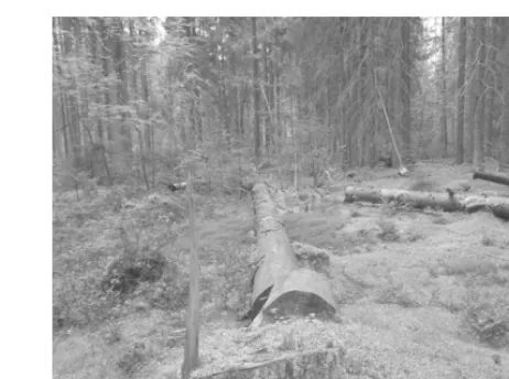
At the present time, cut-to-length logging (CTL) is the primary logging method in European countries. CTL is a mechanized harvesting system in which trees are delimbed and cut to length directly at the stump. Forest residues after the CTL logging are heaps that contain tips, branches, etc. These heaps are close in shape to the circles (Fig. 3). The previously developed LIS method, which was used to estimate distribution of logs and their pieces over the cutting area, cannot be applied for the estimation of the clusters of logging residues after CTL.

In the early 2000s, the authors of the article con-ducted for the first time the study of the possibility of applying the LIS method to estimate logging residues after CTL logging (in the article referred to as »the

clusters of logging residues«) (Karpachev et al. 2010, Karpachev and Scherbakov 2013).

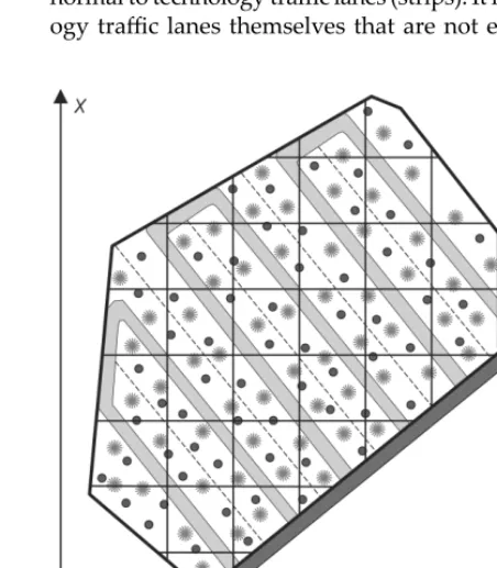
The article (Karpachev et al. 2017) presents the re-sults of studying the LIS method as applied to estimate residues on mathematical models after CTL logging. The obtained results show that the LIS method enables the estimation of different types of residues after CTL logging in terms of the amount, including such com-plex ones as uniform distribution within the technol-ogy traffic lanes (strips) of width b (Fig. 4).

In models, clusters of logging residues were repre-sented as being distributed by strips around a square-cut, regular-shaped area. The sample lines were laid perpendicularly across the whole area. All sample lines were of the same length.

Areal cutting area is not always characterized as a regular polygon. Generally, cutting area may not be

Fig. 1 A graphical explanation of the line-intersect sampling meth-od (LIS)

Fig. 2 Logging residues after logging operation

regular-shaped area (as shown in Fig. 4) but any arbi-trary shape (as shown in Fig. 5). In this case, sample lines are to be of different length (Fig. 5).

The purpose of this paper is to provide information on the LIS method for estimating logging residues in the form of separate heaps – clusters after CTL logging

on a cutting area of any arbitrary shape S (as shown in Fig. 5) with sample li.

In this article, a complex case was considered in terms of its practical application, when only one of the coordinates of the center of clusters (for example, xj)

has uniform distribution, while the other coordinate (for example, yj) is generated in accordance with the

distribution of the strips (Fig. 4). In this case, a differ-ent radius Rj is assigned to each cluster.

This paper:

Þ explains the theory underlying the LIS method for estimating clusters of logging residues on a cutting area with sample lines of different length li

Þ provides basic formulas for estimating the num-ber of cluster using sample lines of different length li

Þ provides simulation models of the heaps with different statistical characteristics and LIS field procedures for estimating the number of clus-ters by using sample lines of different length li

Þ provides basic results of computer simulation of the LIS method for estimating the number of clusters

Þ briefly describes the field-sampling require-ments for the LIS procedures.

2. Theoretical Approach

Let us consider a flat cutting area S. Suppose the area S contains n clusters (Fig. 4), with all the clusters being a circle of the radius R.

The number of clusters on the cutting area S can be estimated by the equation:

N N

n =

å

i

1 ₍₁₎

where:

Ni number of clusters on the cutting area S,

esti-mated by the ith _{sample line}

n number of sample lines.

The number of clusters on the cutting area S can be found using the equation:

i i

i m N

p

= (2) where:

mi number of intersections of clusters with the ith

sample line

Fig. 4 Presentation of clusters on the cutting area

pi probability that the sample line of li intersects

the cluster.

Let all N clusters on the area S have the shape of a circle of the radius R. If the coordinates of the center of the cluster xj, yj are defined as a uniform distribution

on the area S, then the probability that the ith _sample

line of the length li > 2R will intersect the cluster, which

can be equal to (De Vries 1986, Karpachev et al. 2017):

p R l

S

i= i

´ ´ 2

(3)

Equation (3) can also be used provided the coordi-nates of the center of the cluster xj or yj are not defined

as a uniform distribution around the area S (Karpachev and Shcherbakov 2013). For example, the coordinates of the center of clusters were generated in accordance with the distribution of strips along the technology traffic lanes of width b (clusters uniformly distributed along the X-axis and within stripes on the Y-axis, Fig. 4). In this case, we can use equation (3), provided all the sample lines are set normally towards the stripes direction as in Fig. 4 (Karpachev et al. 2017).

Thus, taking into account equation (3), equation (2) can be determined as:

N m S

R l

i i

i = ´

´ ´

2 (4)

Equation (1) with equation (4) can be rewritten as:

N m S R l n S R m l n = ´ ´ ´ æ è

çç ö_ø÷÷ = ´

´ æ

è çç ö_ø÷÷

= =

å

å

n i

i i

n _i

i

1 2 2 1

(5)

In theoretical studies of the LIS method, some as-sumptions have been accepted:

Þ the radii of all clusters are the same, being equal to R. In practice it can only be true for homog-enous forests with uniform tree size and spatial distribution, but it may be invalid for close-to-nature forestry

Þ the coordinates of the cluster centers xj, yj on the

cutting area are determined according to the uniform distribution law.

Due to the accepted assumptions, the theoretical formula may not be accurate enough in practice. In particular, a number of questions arise:

Þ What will be the effect of variability of the clus-ters radii on the estimation accuracy?

Þ What will be the effect of variability of the clus-ters radii on sampling?

Þ What will be the effect of the coordinates distri-bution law of the cluster centers xj, yj on the

es-timation accuracy?

3. Methods

Simulation studies on the LIS method were carried out by various authors (Pickford and Hazard 1978, Pickford and Hazard 1986, Karpachev and Shcherbakov 1990, Karpachev et al. 2010, Karpachev et al. 2017). These studies were aimed at investigating various as-pects of the LIS method. Most simulation research activities on the LIS method studied logging residues that consisted of separate logs. A small number of sci-entific works were devoted to modelling clusters of logging residues after CTL logging (Karpachev et al. 2010, Karpachev et al. 2017). However, these research activities were applicable to sample lines of the same length.

The present paper considers a cutting area S with all sample lines of different length. Such model can be found in Fig. 5, and it complies with the field condi-tions to a better extent.

However, the LIS method practical application, us-ing the scheme in Fig. 5, faces a number of difficulties. In particular, it is hard to lay sample lines that are normal to technology traffic lanes (strips). It is technol-ogy traffic lanes themselves that are not easy to be

determined in a forested area. When applied, it is easier to lay sample lines along the arbitrarily chosen direction. In this case, there is a risk of sample lines coinciding with technology traffic lanes, which might lead to a significant variance, thus increasing the num-ber of the required sample lines. To avoid that, sample lines may be laid perpendicularly in shape of a grid, as shown in Fig. 6. We have studied this scheme based on mathematical models, and the findings are pre-sented in this article.

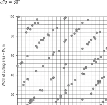
The developed mathematical model of clusters and sample lines on the cutting area differed from the one in Fig. 6. In the mathematical model, the cutting area was assigned as a plane rectangular shape of size LхH (Fig. 7–10).

Based on the field measurement data (Karpachev et al. 2010, Karpachev and Shcherbakov 2013), the fol-lowing assumptions for the clusters of logging resi-dues were accepted and used in the mathematical model:

Þ shape of the clusters is a correct circle with the variable radius Rj

Þ variation of the clusters radii is described by the normal distribution law

Þ location of clusters on cutting area was taken as distributed by strips at an angle alfa to the Y -axis

Þ coordinate xcj of residues spots was assigned

ac-cording to the normal distribution law on the interval [0, L]

Þ coordinate ycj was assigned according to the

nor-mal distribution law within the width of their strips b.

In practice, it was the most difficult to determine the shape and size of the clusters of logging residues. Our experience (Karpachev and Shcherbakov 2013) has shown that it is quite well to present the clusters as circles of variable radius Rj. In practice, we measured

the perimeters of the logging residues and then calcu-lated the radii (Fig. 15). The mean radius of the clusters R was determined from field measurement data.

The coordinates of the center of clusters xcj, ycj were

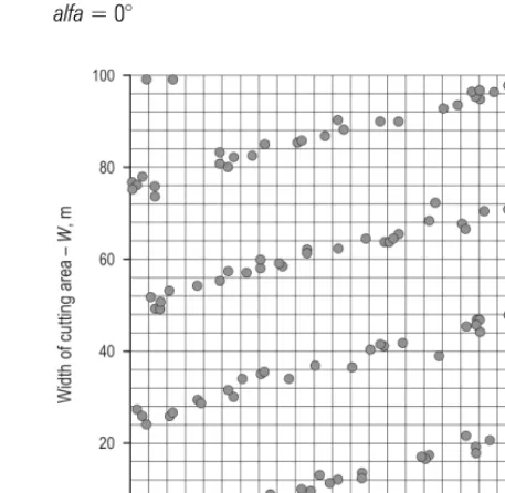
generated in accordance with the distribution by strips along the X-axis. In experiments, the angles be-tween strips and the X-axis varied from 0 to 45° with 15° step. To gather statistics, we have generated hun-dreds of cluster models. Examples of generating the clusters with different angles can be found in Fig. 7 through 10.

The sample lines of different length were assigned, mutually perpendicular and parallel to the coordinate

axes X, Y (Fig. 11). This grid of sample lines was placed on each generated cluster model.

The mathematical model enabled to simplify the modelling procedure, where the main idea of estimat-ing clusters by sample lines of different length still applied.

The length lj of the sample line was a random

vari-able taken upon the condition lj > Ri.

Fig. 8 An example of generating stripes of clusters with the angle

alfa = 15°

Fig. 7 An example of generating stripes of clusters with the angle

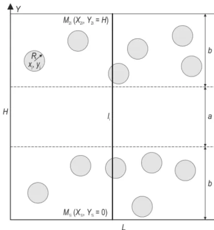
Each sample line was defined by the points of its beginning M1i (X1i, Y1i) and end M2i (X2i, Y2i). The

mod-el generated several sets of sample lines on the cutting area. There were four types of lines in each set:

1. Coordinates of the 1st _{type of lines were M} 1i (X1i =

0, Y1i); M2i (X2i, Y2i = Y1i). Coordinates Y1i, X2i were

assigned according to the distribution law on the intervals [0, H] and [2Rmax, L], respectively

2. Coordinates of the 2nd _{type of lines were M} 1i (X1i,

Y1i = 0); M2i (X2i = X1i, Y2i). Coordinates X1i, Y2i

were assigned according to the distribution law on the intervals [0, L] and [2Rmax, H], respectively

3. Coordinates of the 3rd _{type of lines were M} 2i (X2i =

L, Y2i); M1i (X1i, Y1i = Y2i). Coordinates Y2i, X1i were

assigned according to the distribution law on the intervals [0, H] and [0, L – 2Rmax], respectively

4. Coordinates of the 4th _{type of lines were M} 2i (X2i,

Y2i = H); M1i (X1i = X2i, Y1i). Coordinates X2i, Y1i were

assigned according to the distribution law on the intervals [0, L] and [0, H – 2Rmax], respectively.

An example of clusters generation within six strips (angle alfa = 15°) with the set of four sample lines of different length is shown in Fig. 11.

The maximum radius Rmax was defined by the

for-mula:

3 Standard deviation

Rmax R= + × (6)

where:

R the mean radius of the clusters.

In the model, we used the mean value of the radius R = 3 m.

The fact of intersection of jth _{cluster with i}th _sample

line for 1st _{type of lines was defined according to the}

following algorithm.

1. The ith _{sample line intersects j}th _{cluster, provided}

it meets the logical condition:

Fig. 10 An example of generating stripes of clusters with the angle

alfa = 45°

Fig. 9 An example of generating stripes of clusters with the angle

y_cj R_j Y_1i y_cj R_j _and_ X_2i x_cj (7)

2. If condition (7) fails to be met, then the intersec-tion can still be appliied provided an addiintersec-tional logical condition is fulfilled (Fig. 12):

y_cj R_j Y_1i y_cj R_j _and_ X_2i x_cj _and_ r_ij R_j

y_cj R_j Y_1i y_cj R_j _and_ X_2i x_cj _and_ r_ij R_j (8)

Equations (7) and (8) may be united into a single logical condition:

y_cj R_j Y_1i y_cj R_j _and_ X_2i x_cj _and_ r_ij R_j

y_cj R_j Y_1i y_cj R_j _and_ X_2i x_cj _and_ r_ij R_j (9) where:

= − 2+ − 2

ij ( cj 2i) ( cj 2i)

r x X y Y (10)

Likewise, logical conditions of sample line intersec-tion with the cluster for all other types of line can be obtained.

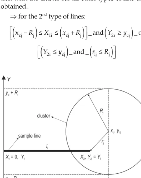
Þ for the 2nd _{type of lines:}

x_cj R_j X_1i x_cj R_j _and

(

)

Y_2i y_cj _and_ r_ij R_j (11)

where:

r_ij= (x_cj-X_2i)2+(y_cj-Y_i)

2 2 (12)

Þ for the 3rd _{type of lines:}

y_cj R_j Y_1i y_cj R_j _and

(

)

X_1i x_cj _and_ r_ij R_j (13)

where:

r_ij= (x_cj-X_1i)2+(y_cj-Y_i)

1 2 (14)

Þ for the 4th _{type of lines:}

x_cj R_j X_1i x_cj R_j _and

(

)

Y_1i y_cj _and_ r_ij R_j (15) where:

r_ij= (x_cj-X_1i)2+(y_cj-Y_i)

1 2 (16)

Estimation of the number of clusters was conduct-ed using the algorithm describconduct-ed above. Estimation procedures were implemented in Delphi 7 program. In developing the computer program, we used com-mon approaches used earlier (Karpachev et al. 2017). The program interface of the clusters estimation by the LIS method is shown in Fig. 13.

Fig. 12 Condition of intersection of the ith _{sample line with the j}th

cluster for the 1st _{type of lines}

Fig. 13 Program interface for clusters estimation using LIS

Table 1 Results of the LIS simulation (used mean radius from intersected clusters with all sample lines)

Angle of strips alfa True number of clusters Mean length of lines, m

Experimental (estimation from model) Theoretical (by formula)

Mean number of intersections of clusters per line Mean radius from intersected clusters with all sample lines, m Number of clusters Variance of the number of intersections of clusters per line Error estimates of the number of clusters, % Required number of sample lines Required number of sample lines Mean number of intersections of clusters per line Variance of the number of intersections of clusters per line

0 30 58.15 0.95 3.71 22 2.18 26.40 231 96 0.96 0.93 0 72 56.92 2.09 3.34 55 8.65 23.77 191 41 2.25 2.18 0 124 57.92 4.27 3.96 93 21.87 24.89 115 23 3.95 3.82 15 40 57.11 1.28 3.83 29 1.11 27.01 65 74 1.26 1.21 15 78 57.13 2.47 3.71 58 3.81 25.37 60 37 2.45 2.37 15 122 56.88 4.14 3.98 91 11.47 25.10 64 24 3.81 3.69 30 45 57.45 1.33 3.47 33 1.59 25.73 85 65 1.42 1.38 30 80 57.49 2.77 3.64 66 4.15 17.38 80 36 2.53 2.45 30 123 57.33 4.02 3.79 92 8.76 24.82 52 24 3.88 3.75 45 44 57.77 1.37 3.65 33 1.71 26.00 87 66 1.40 2.39 45 77 58.02 2.54 3.82 57 4.91 25.56 72 37 2.46 2.39 45 121 57.34 3.82 3.73 89 6.16 26.24 40 24 3.78 2.39

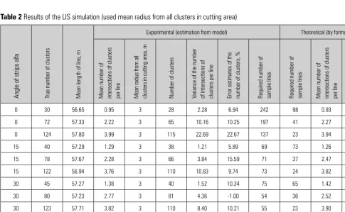
Table 2 Results of the LIS simulation (used mean radius from all clusters in cutting area)

Angle of strips alfa True number of clusters Mean length of line, m

Experimental (estimation from model) Theoretical (by formula)

Mean number of intersections of clusters per line Mean radius from all clusters in cutting area, m Number of clusters Variance of the number of intersections of clusters per line Error estimates of the number of clusters, % Required number of sample lines Required number of sample lines Mean number of intersections of clusters per line Variance of the number of intersections of clusters per line

4. Results and Discussion

The LIS simulation results are shown in Table 1 and Table 2. All results are given with a 20% accuracy rate.

Table 1 shows that the radius estimation R (mean radius from intersected clusters with all sample lines) exceeds the true mean value R = 3 m (mean radius from all clusters in cutting area). For example, for both strips orientation angle of 30° and the true number of clusters = 45 R = 3.47 m, which exceeds the true mean value by 15.7%.

Exceeding of the mean radius compared to the true mean radius for all angles and different number of spots can be seen in Fig 14. The mean value of ra-dius estimation was R = 3.71 m, which exceeds the true mean value R by 24%. Exceeding of the value estimation can be explained by the fact that, in the model, the estimation was defined using cluster sam-ples intersected by sample lines. Practically, such ap-proach proved to be the most suitable (Fig. 15). How-ever, according to Eq. 3, the probability that the sample line will intersect the cluster depends on the radius R. As a result, the radius R estimation was de-fined as too excessive for all angles and numbers of clusters (Fig. 14).

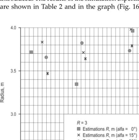
To assess the way the cluster radius affects the es-timation accuracy of the numbers of clusters, the con-stant value of the radius for all clusters (R = 3 m) was introduced. The results of the simulation experiments are shown in Table 2 and in the graph (Fig. 16). As

shown by the graph (Fig. 16), the discrepancy be-tween the theoretical and experimental results for the radius estimations exceeded a 20% error. It should be emphasized that, for the constant value of the radius (R = 3 m), the discrepancy between the theoretical and experimental results exceeded the 20% error only in one case. The mean error was 9.3%.

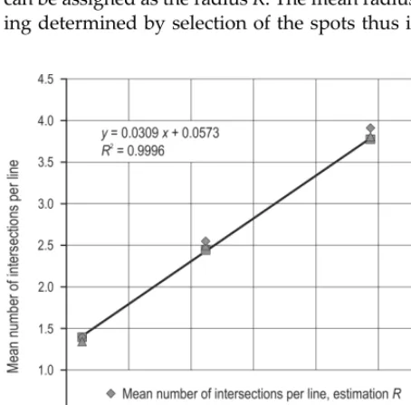
It is interesting to analyze the mean numbers of intersections per line. An example of the results of simulation experiments (Table 1, Table 2) with the strip angle alfa = 45° can be found in Fig. 17. The experimen-tal data almost coincide with the theoretical data.

Fig. 14 Dependence of cluster radius estimation on the number of clusters for different angles of strips

Fig. 15 Measuring the perimeter of the cluster

An example of the dependence of the required number of sample lines on the number of clusters is shown in Fig. 18 (strip angle alfa = 45°). For compari-son, in Fig. 18 the theoretical curve can be found for clusters with the uniform distribution law. As shown by the graph, the required number of sample lines for the clusters estimation that were distributed with strips (Fig. 10) was twice to three times larger than for uniformly distributed clusters.

That can be explained by the fact that the variance of the average number of intersection of clusters with the lines will be higher than for uniformly distributed clusters.

For example, for 121 clusters with strip angle alfa = 45° (Table 1, Table 2), the theoretical number of sample lines is 24 lines. The required number of sample lines, calculated by the results of the experiments, amount-ed to 40 lines (estimation R) and 42 lines (R = 3 m).

5. Conclusion and Practical

Recommendations

Estimation of the number of clusters on the cutting area of the arbitrary shape S can be made according to Eq. 5.

While using Eq. 5, the mean radius of the clusters can be assigned as the radius R. The mean radius, be-ing determined by selection of the spots thus

inter-sected by the sample lines, resulted in the mean radius estimation that exceeds the true mean radius by 24% in simulation experiments. That can be explained by the fact that, according to the formula (Eq. 3), it is more likely for a larger radius to be intersected when com-pared to a smaller one.

Practically, in the case of determining the mean radius from a sample of clusters intersected by the laid lines, a correction should be made for the mean radius estimation.

Estimation of the radius does not depend on the number of clusters and angles of strips.

If the sample lines cross the cutting area (parallel to the Y-axis) and are equal to the width of the area, then the probability that the sample line will intersect the cluster can be determined by equation Eq. 3.

Estimation of the number of clusters should be done according to the results of the intersections of the clusters with n sample lines according to the formula (Eq. 5). The required number of sample lines can be determined according to statistics formula.

Simulation experiments were carried out for 4 types of clusters as shown in Table 1, Table 2 and some of them in Fig. 14, 16, 17 and 18.

The results of simulation showed that, when the location of the sample lines are across the area (Fig. 14, 16), i.e., across the stripes with clusters, the results comply with the theoretical formulas. Discrepancies remain within a 20% error. This is due to the fact that,

Fig. 17 Dependence of the required number of sample lines on the mean number of intersections of clusters with sample line (strip angle alfa = 45°)

in this case, the estimation is only affected by the x -coordinate of the clusters.

When the location of the sample lines are along the cutting area (along the strips with clusters), the results failed to comply with the theoretical formulas. The discrepancies can exceed a 100% error. A significant discrepancy is explained by the fact that the estima-tion, in this case, is only affected by the y-position of the center of the cluster, which is distributed within the stripe. A number of the sample lines go through the stripes with a large number of intersections with the clusters, but the rest of the lines get between the strips, where there are no intersections of the lines with the clusters. This will clearly lead to an increase of variance (or standard deviation), which will corre-spondingly increase the required number of sample lines.

For clusters with coordinates x, y distributed by the uniform law around the cutting area, it is possible to carry out a sample line across the area and along the area. In this case, in practice, the sample lines can be drawn either way (along or across the cutting area).

For clusters distributed around the cutting area inside the stripes, the sample lines should be laid across the stripes. The required number of the sample lines can be predetermined according to statistics for-mula and can be clarified during the field measure-ment process using the graph (Fig. 17 and Fig. 18).

6. References

Bailey, G.R., 1969: An evaluation of the line-intersect method of assessing logging residue. Inform. Rep. VP-X-23, Can. Dep. Fish. Forest., Forest Prod. Lab., Vancouver, B.C., 36 p. Bailey, G.R., 1970: A simplified method of sampling logging residue. Forest. Chron. 46(4): 288–294. https://doi. org/10.5558/tfc46288-4

Bailey, G.R., Lefebvre, E.L., 1971: Estimating volume distri

-butions of logging residue from intersect-sampled data. Bi-Mon. Res. Notes 27: 4–5.

Bate, L., Torgersen, T., Wisdom, M., Garton, E., 2009: Biased estimation of forest log characteristic using intersect diam-eters. Forest Ecology and Managment 258(5): 635–640. https://doi.org/10.1016/j.foreco.2009.04.042

Bell, G., Kerr, A., McNickle, D., Woollons, R., 1996: Accuracy of the line intersect method of post-logging sampling under orientation bias. Forest Ecology and Management 84(1–3): 23–28. https://doi.org/10.1016/0378-1127(96)03773-5 Brown, J.K., 1974: Handbook for inventorying downed woody material. Gen. Tech. Rep. INT-16. Ogden, UT: U.S. Department of Agriculture, Forest Service, Intermountain Forest and Range Experiment Station, 24 p.

Brown, J.K., Roussopoulos, P.J., 1974: Eliminating biases in

-the planar intersect method for estimating volumes of small fuels. Forest Science 20(4): 350–356.

Dalkey, N., Olaf, H., 1963: An Experimental Application of the DELPHI Method to the Use of Experts. Management Science 9(3): 458–467. https://doi.org/10.1287/mnsc.9.3.458

De Vries, P.G., 1973: A general theory on line intersect sam

-pling with application to logging residue inventory. Mad

-elingen Landbouw Hogeschool. No 73–11, Wageningen, Netherlands, 23 p.

De Vries, P.G., 1974: Multi-Stage Line Intersect Sampling.

Forest Science 20(2): 129–133. https://doi.org/10.1093/forest

-science/20.2.129

De Vries, P.G., 1979: Line Intersect Sampling: Statistical Theory, Applications and Suggestions for Extended Use in Ecological Inventory. In Sampling Biological Populations.

Editors G.M. Cormack, G.P. Patil, and D.S. Robson. Interna

-tional Coop. Publishing House. Fairland, Maryland, Statisti

-cal Ecology Series, Vol. 5: 1–7

De Vries, P.G. 1986: Sampling Theory for Forest Inventory. Springer-Verlag. New York, 399 p. (Chapter 13, pages 242– 279, deals specifically with line intersect sampling.)

Ghaffariyan, M.R., 2013: Remaining slash in different har

-vesting operation sites in Australian plantations. Silva Bal-canica 14(1): 83–93.

Ghaffariyan, M.R., Brown, M., Acuna, M., 2012: Sampling methodology for left-slash assessment in collecting forest biomass. Forest Energy Blog, October 31, 2012 at http://blog. forestenergy.org.

Ghaffariyan, M.R., Jenkin, B, Mitchell, R., Brown, M., 2016:

Quantitative and Qualitative Assessment of Timber Harvest

-ing Residues: A Case Study of a Balsa Plantation in Papua

New Guinea. IUFRO Research Group 3.08 Small-scale For

-estry Conference. Small-scale and Community For-estry and the Changing Nature of Forest Landscapes, October 11–15, 2015. Sunshine Coast, Australia. Conference Proceedings, 65–77.

Harmon, M.E., Franklin, J.F., Swanson, F.J., Sollins, P., Greg

-ory, S.V., Lattin, J.D., Anderson, N.H., Cline, S.P., Aumen,

N.G., Sedell, J.R., Lienkaemper, G.W., Cromack, K.Jr., Cum

-mins, K.W., 1986: Ecology of coarse woody debris in temper

-ate ecosystems. In: MacFadyen, A., Ford, E.D., eds. Advanc

-es in ecological r-esearch. Orlando, FL: Academic Pr-ess, Inc.: 15: 133–302.

Hazard, J.W., Pickford, S.G., 1984: Cost Functions for the Line Intersect Method of Sampling Forest Residue in the Pacific Northwest. Canadian Journal of Forest Research 14(1): 57–62. https://doi.org/10.1139/x84-012

Howard, J.O., Ward, F.R., 1972: Measurement of logging residue – alternative applications of the line intersect meth-od. USDA For. Serv. Res. Note PNW-183, 8 p.

Karpachev, S.P., Shcherbakov, E.N., 1990: Modelling on computer resource estimates and parameters of logging residues by the method of line intersections – M. Scientific. Tr., Moscow State Forest University, 226, 4 p.

Karpachev, S.P., 2005: Quantitative estimation of the envi

-ronmental impact of the traditional use of forest rivers for

floating timber transport: estimating of the volume of sunk

-en timber in rivers. Session 013, XXII IUFRO World Con

-gress. Forests in the Balance: Linking Tradition and Technol

-ogy, August 8 – 13.

Karpachev, S.P., 2006: Quantitative estimation of the envi

-ronmental impact of the traditional use of forest rivers for

floating timber transport: estimating of the volume of sunk

-en timber in rivers. 2nd _{International Conference on}

Environ-mentally-Compatible Forest Products. Fernando PessoaU-niversity. Oporto, Portugal 20 – 22 September.

Karpachev, S.P., 2008a: The quantitative estimation of the rest residuals as biomass to produce bioenergy for local in-dustry and villages in forest regions of Russia. Proceedings World Bioenergy, The Swedish Bioenergy Association, Sve-bio, Torsgatan 12, SE-111 23 Stockholm, Sweden, 408–410. Karpachev, S.P., 2008b: The quantitative estimation of the-forest residuals as biomass for bio-energy for local industry

and villages in forest regions of Russia. FORMEC. 41. Inter

-national Symposium in Schmallenberg, Germany June, 2–5, Gross-Umstadt, 51–56.

Karpachev, S.P., 2009: Operative Method for Quantitative

and Qualitative Estimation of Forest Residuals After Har

-vesting Logging Operations as Biomass for Bioenergy, Bio

-energy, Sustainable Bioenergy Business, 4th _{International}

Bioenergy Conference and Exhibition, August 31 –

Septem-ber 4, Available at: http://www.hedon.info/docs/Bioener

-gy2009_progamme.pdf.

Karpachev, S.P., Shcherbakov, E.N., 2009: Basic research of the probabilistic features of the estimation of the heaps of

the forest residuals by the linear intersection method. Mos

-cow State Forest University Bulletin – Lesnoj Vestnik 67(4): 97–99.

Karpachev, S.P., Shcherbakov, E.N., Slinchencov, A.N., 2010:

Quantification of logging residues after CTL logging by har

-vesters. The lesopromyshlennik journal 4(56): 29–31. Karpachev, S.P., Shcherbakov, E.N., 2013: Statistical evalua-tion of the quantity and quality of accumulaevalua-tions of wood produced in forest areas and water bodies. Monography, Moscow State Forest University, 132 p.

Karpachev, S.P., Zaprudnov V.I., Bykovskiy, M.A., Scherba

-kov E.N., 2017: Quantitative Estimation of Logging Residues

by Line-Intersect Method. Croatian journal of forest engi

-neering 38(1): 33–45.

Nemec, A.F.L., Davis, G., 2002: Efficiency of six line intersect sampling designs for estimating volume and density of coarse woody debris. Res. Sec., Van. For. Reg., B.C. Min. For., Nanaimo, B.C. Tec. Rep. TR-021/2002, 12 p.

Marshall, P.L., Davis, G., LeMay, V.M., 2000: Using Line In

-tersect Sampling for Coarse Woody Debris. Technical Report TR-003 March, Research Section, Vancouver Forest Region, BCMOF, 34 p.

O’Hehir, J., Leech, J., 1997: Logging residue assessment by line intersect sampling. Australian Forestry 60(3): 196–201. https://doi.org/10.1080/00049158.1997.10676142

Pickford, S.G., Hazard, S.W., 1978: Simulation Studies on Line Intersect Sampling of Forest Residue. Forest Science 24(4): 469–483. https://doi.org/10.1093/forestscience/24.4.469 Van Wagner, C.E., 1968: The Line Intersect Method in Forest Fuel Sampling. Forest Science 14(1): 20–26. https://doi. org/10.1093/forestscience/14.1.20

Van Wagner, C.E., Wilson, A.L., 1976: Diameter Measure

-ment in the Line Intersect Method. Forest Science 22(2): 230–232. https://doi.org/10.1093/forestscience/22.2.230

Van Wagner, C.E., 1982: Practical Aspects of the Line Inter

-sect Method. Information Report PI-X-12. Petawawa Na

-tional Forestry Institute, Canadian Forest Service, 11 p. Warren, W.G., Olsen, P.F., 1964: A Line Intersect Technique for Assessing Logging Waste. Forest Science 10(3): 267–276. https://doi.org/10.1093/forestscience/10.3.267

Woldendorp, G., Keenan, R., Barry, S., Spencer, R., 2004: Analysis of sampling methods for coarse woody debris. For-est Ecology and Management 198(1–3): 133–148. https://doi. org/10.1016/j.foreco.2004.03.042

Received: February 12, 2018 Accepted: June 27, 2019

Authors’ addresses:

Prof. Sergey P. Karpachev, PhD. * e-mail: [email protected]

Prof. Vjacheslav I. Zaprudnov, PhD. e-mail: [email protected]

Assoc. prof. Maksim A. Bykovskiy, PhD. e-mail: [email protected]

Engineer Irina P. Karpacheva e-mail: [email protected] Mytischi Branch of Bauman Moscow State Technical University 1st Institutskaya street 1

141005 Mytischi, Moscow region RUSSIA