Eric Canc`es & Jean-Fr´ed´eric Gerbeau, Editors DOI: 10.1051/proc:2005010
A PENALTY METHOD FOR THE SIMULATION OF FLUID - RIGID BODY
INTERACTION
Jo˜
ao Janela
1, Aline Lefebvre
2and Bertrand Maury
2Abstract. We present here a method to simulate the motion of a rigid body in a fluid. The method is based on a variational formulation on the whole fluid/solid domain, with some constraints on the unknown and the test functions. These constraints are relaxed by introducing a penalty term, which leads to a minimization problem over unconstrained functional spaces. This makes the method straight-forward to implement from any finite element Stokes/Navier-Stokes solver. It is shown that, as the penalty parameter goes to infinity, we recover the coupled fluid-solid equations. We apply this approach to a simplified 2D model of the aortic valve.
R´esum´e. Nous pr´esentons ici une m´ethode de simulation du mouvement d’un corps rigide dans un fluide. Cette m´ethode est bas´ee sur une formulation variationnelle sur tout le domaine fluide/solide, avec des contraintes sur l’inconnue et sur les fonctions test. On relaxe ces contraintes en introduisant un terme de p´enalisation, qui conduit `a un probl`eme de minimisation sur des espaces fonctionnels non contraints. Ainsi, tout solveur ´el´ements finis pour Stokes/Navier Stokes permet de programmer ais´ement cette m´ethode. On montre que, quand le param`etre de p´enalisation tend vers l’infini, on retrouve le syst`eme d’´equations coupl´ees fluide/solide. Cette approche est appliqu´ee `a un mod`ele 2D simplifi´e de la valve aortique.
Introduction
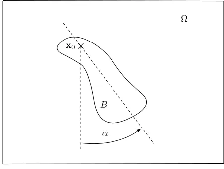
We consider a connected bounded, regular domain Ω ⊂ R2 and we denote by B a subset of Ω strongly contained in Ω. We shall restrict ourselves to the case where B is connected (see figure 1), but one can easily generalize to any domainB with several connected components. We suppose that Ω\B¯ is filled with a Newtonian fluid governed by the Navier-Stokes equations and thatB is a rigid inclusion in Ω. We suppose that Bis attached at one of its pointsx0. We shall apply our approach to a situation where the rotating rigid body is submitted to an angular pull-back moment.
Numerical simulations of such a problem can be carried out in many different ways, which we may classify into two main classes. The first one relies on a moving mesh which fits the moving part of the boundary (see e.g. [4], [5], and [7]). In the second approach, the whole domain is covered by a static mesh. Those methods are known asfictitious domain or embedded domain methods, as the actual computational domain (the fluid component) is extended to a larger domain which covers the area of interest (zones which are likely to be occupied by the fluid). To our knowledge, all fictitious domain approaches which have been applied to problems like the one we consider are based on Lagrange multipliers (see [3]), which enforce the velocity in the solid part
1CEMAT, Instituto Superior T´ecnico and Departamento de Matem´atica, ISEG, Lisbon, Portugal; e-mail:[email protected]
2Laboratoire de Math´ematiques, Universit´e Paris Sud, Orsay, France; e-mail: [email protected] & [email protected]
c
EDP Sciences, SMAI 2005
x0
Ω
α B
Figure 1. Model problem
to identify to the velocity of the rigid body. We propose here a penalty method to handle the rigid motion. As the penalty changes the stiffness operator, we loose an advantage of the Lagrange multiplier method, which is the possibility to use Fast Fourier Transform-like solvers. On the other hand, this method can be implemented straightforwardly on a general Finite Element solver like FreeFem++ (see [1]), which we used to run numerical experiments.
1.
Continuous problem and Variational Formulation
For the sake of simplicity, we will consider here homogeneous Dirichlet conditions on∂Ω. The fluid obeys Navier-Stokes equations in Ω\B¯ = Ω\B¯(t) at every timet, and the body motion follows the Newton law, which reduces here to an equation on the angular velocity around x0. Those equations are coupled by hydrodynamic forces exerted by the fluid on the solid. Finally, viscosity imposes no-slip conditions on the boundary ofB: at each point of∂B, the velocity on the fluid side is equal to the velocity on the rigid side.
We denote byω = ˙θ the angular velocity of B, so that we have to find a velocity fieldu= (u1, u2) defined in Ω\B¯,ω∈Rand a pressure field p defined in Ω\B¯ such that :
ρfDu
Dt −µu+∇p = ff in Ω\B¯
∇ ·u = 0 in Ω\B¯
u = 0 on∂Ω
u(x) = ω(x−x0)⊥ on∂B
Jx0ω˙ = B(x−x0)⊥·fB−∂B(x−x0)⊥·σnds
(1)
whereff andfB are the external forces exerted on the fluid and the rigid body respectively,ρf andρBare their respective densities, µ is the viscosity of the fluid, nis the external normal to Ω\B¯, σ is the Cauchy stress tensor, Jx0 is the kinetic momentum ofB at pointx0 andDu/Dtis the total derivative ofu:
σ= 2µD(u)−pId and D(u) =∇u+ (∇u) T
Jx0 =
BρB|
x−x0|2, Du
Dt = ∂u
∂t + (u· ∇)u, andx⊥ denotes (−x2, x1).
Our first step will consist in establishing a variational formulation easily tractable from the numerical point of view, i.e. involving functions which are defined on the whole domain Ω. This can be achieved by prescribing the constraints on both the unknown velocity field and its test counterpart, at (almost) every time. In what follows, we consider the problem at a given timet, and we drop the dependence of the domain Ω\B¯ upont, in order to alleviate notations. We introduce the following spaces:
Kx0=
u∈H01(Ω)2,
D u= 0
, Kx0,∇={u∈Kx0,∇ ·u= 0},
KB ={u∈H01(Ω)2,∃(V, ω)∈R2×Rs.t. u=V+ω(x−x0)⊥ a.e. in B},
whereD is a disc included inB and centered atx0. As forKB, which is the space of velocity fields which do not deformB, it can be written
KB={u∈H01(Ω)2,D(u) = 0 a.e. onB}.
Note thatKBdepends on the position ofB, and therefore it is likely to vary over time. For the sake of clarity, we shall occasionally denote an element ofKB by expliciting the real degrees of freedom: U= (u,V, ω)∈KB. Note that ifU= (u,V, ω)∈KB∩Kx0 thenV is necessarily equal to zero, which expresses the fact thatB is
fixed atx0. We nevertheless keepVas an unknown, because both contraints will be dealt with in different ways in actual computations. The subspaces we have introduced are closed inH01(Ω)2 and they are consequently
Hilbert spaces for theH1norm. Let nowU= (u,V, ω)∈Kx0∩KB be a solution of the problem at a certain
timet. We multiply the Navier Stokes equation by ˜U= (˜u,V˜,ω˜)∈Kx0∩KB and integrate it over Ω\B¯ :
Ω\B¯ρf
Du Dt ·u˜−µ
Ω\B¯∆u·˜
u+
Ω\B¯∇p·˜
u=
Ω\B¯
ff·u˜. Integration by parts gives
Ω\B¯ρf
Du
Dt ·u˜+ 2µ
Ω\B¯D(u) :D(˜u)−
Ω\B¯p∇ ·˜
u−
∂(Ω\B¯)σ
n·u˜ =
Ω\B¯
ff·u˜. Then, using the fact that ˜u= ˜ω(x−x0)⊥ inB and using the boundary conditions on∂B, we obtain :
Ω\B¯ρf
Du
Dt ·u˜+ Jx0ω˙ω˜+ 2µ
Ω\B¯D(u) :D(˜u)−
Ω\B¯p∇ ·˜
u=
Ω\B¯
ff·u˜+
B fB·u˜.
Since ˜u∈KB, the third term can be written over Ω and, sinceD(u) = 0 implies∇ ·u= 0, so can be the fourth
one :
Ω\B¯ρf Du
Dt ·u˜+ Jx0ω˙ω˜+ 2µ
ΩD(u) :D(˜u)−
Ωp∇ ·˜
u=
Ω
f·u˜
wheref =ffχΩ\B¯+fBχB. Finally, using thatu=ω(x−x0)⊥ and ˜u= ˜ω(x−x0)⊥ inB we can prove that
Jx0ω˙ω˜ =
BρBω˙ω˜|
x−x0|2=
BρB Du
which leads to the variational formulation Ωρ Du
Dt ·u˜+ 2µ
ΩD(u) :D(˜u)−
Ωp∇ ·˜
u=
Ω
f·u˜ ∀˜u∈Kx0∩KB,
Ωq∇ ·
u= 0 ∀q∈L2(Ω),
(2)
whereρ=ρfχΩ\B¯+ρBχB.
2.
Time discretization and penalty Method
2.1.
Time discretization
We use the method of characteristics to discretize the total derivative. Note that, as ρ is constant along trajectories, we have
ρDu Dt =
Dρu Dt .
We denote byXn(x) an approximation ofX(x,(n+ 1)∆t, n∆t) whereXis the characteristic associated to u. It can be expressed as the solution to the following problem:
∂X
∂τ (x, t, τ) =u(X(x, t, τ), τ) X(x, t, t) =x
So, the time discretized problem is written at each time step :
un+1∈Kx0∩KBn+1 and pn+1∈L2(Ω)
α
Ωρ
n+1un+1·u˜+ 2µ ΩD(u
n+1) :D(˜u)− Ωp
n+1∇ ·u˜
=αΩ(ρnun)◦Xn·u˜+Ωfn+1·u˜ ∀u˜ ∈Kx0∩KBn+1,
Ωq∇ ·
un+1= 0 ∀q∈L2(Ω),
(3)
where α= 1/∆tandBn+1 is computed usingθn+1=θn+ ∆tωn.
2.2.
Penalty method
The previous formulation involves test functions in the constrained space of rigid motions onB. In order to relax this constraint, and make the algorithm easily implementable, we propose here a penalty method. Note that the rigid motion constraint can also be taken into account by mean of tensorial Lagrange multipliers, as it is done in [9].
Firstly, we write problem (3) as a minimization problem:
un+1∈Kx0,∇∩KBn+1
Jn(un+1) = min
v∈Kx0,∇∩KBn+1
Jn(v) (4)
where
Jn(v) = α 2
Ωρ
n+1v2+µ
ΩD(v) :D(v)−α
Ω(ρ
nun)◦Xn·v−
Ω
Problems (3) and (4) are equivalent, in the sense that (un+1,pn+1) solves (3) implies thatun+1is a solution to (4), and ifun+1is a solution to (4), there exists pn+1such that (un+1,pn+1) is a solution to (3). Uniqueness of the pressure is of course out of reach, as it is clearly underdetermined within the rigid body. Existence and uniqueness of a solution to (4) is a direct consequence of Korn’s second inequality (see [8]) and Lax Milgram theorem.
We are now going to approach that minimization problem with another minimization problem by penalizing the rigid motion constraint:
un+1∈Kx0,∇ Jn(un+1) = min
v∈Kx0,∇
Jn(v) (5)
where
Jn(v) = Jn(v) +1
Bn+1D(v) :D(v)
Note that, as before, we can prove that problem (5) admits a unique solution.
2.3.
Convergence of the penalty method
We establish here the convergence of the penalty method at each time step. To that purpose, we introduce the following abstract framework. We denote byV a Hilbert space,aandbtwo bilinear, symmetric and continuous forms onV, a being coercive and b being positive (b(u,u)≥0), and φa linear form on V. We consider the following problems :
u∈ {w∈V s.t. b(w,w) = 0} J(u) = min
v∈{w∈V s.t. b(w,w)=0}J(v)
(6)
and
u∈V J(u) = min
v∈V J(v)
(7)
where
J(v) = 1
2a(v,v)− φ,v, J(v) = J(v) + 1
b(v,v) It is shown in [6] that :
Theorem 1. If uandu are respectively solution to problem (6) and problem (7) then u tends (strongly) to
u as goes to 0. Moreover, if b can be written b(u,v) = (Ψu,Ψv)Γ where Γ is a Hilbert space and Ψ is a continuous linear mapping fromV toΓ, with closed range, we have the following error estimate :
∃C >0 s.t. |u−u| ≤C
Our problem fits into this framework, with (up to multiplicative constants)
V =Kx0,∇
a(u,v) =Ωu·v+ 2µΩD(u) :D(v) b(u,v) =BD(u) :D(v)
Lemma 1. The mapping u −→ D(u)|B is linear and continuous from Kx0,∇ to L2(B)
4
, and its range is closed.
Proof. We consider a sequence (un)n∈N ∈ Kx0,∇ such that D(un)|B tends to z in L2(B)
4
as n goes to infinity. We are going to buildu∈Kx0,∇ such thatz=D(u)|B. We consider ¯un∈Kx0,∇(B), the orthogonal projection ofun|B on (Kx0,∇(B)∩KB)⊥. Since ¯un is orthogonal to the space of rigid motions onB we have
(see [8]) :
u¯nH1(B)≤CD(¯un)L2(B)
AsD(¯un) =D(un)|B, it follows that (¯un)n is bounded in H1(B). We now want to extend ¯un over Ω. Since
∂B¯un·n= 0, we can construct (see [2]) a divergence free extension on Ω bounded in H1(Ω) by ¯unH1(B). Up to an extracted subsequence, this last sequence converges weakly tou∈Kx0,∇ as n goes to infinity and it follows immediately thatz=D(u)|B.
3.
Numerical results
In this section we describe how the penalty method introduced in section 2.3 can be used to simulate the motion of an idealized aortic valve.
3.1.
Description of the model
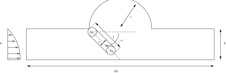
In this somewhat over-simplified model, the “valve” is supposed to be rigid. We furthermore assume it is rotating aroundx0, center ofD1. The geometry outlined in Figure 2 arises from some geometric simplifications
of the real physical geometry of the aortic valve that can be found in [10]. The elastic complex behaviour that
v h
6h D1
D2
r
e α
Figure 2. Geometry of the model problem
makes the valve return to an equilibrium position has been modeled adding a pull-back moment. More precisely, we added an external force term, acting onD2, whose moment is proportionnal to α−αeq where αeq is the angle of equilibrium. Therefore, the external force term including gravity and pull-back moment is :
f1= C
(α−αeq) sinαχD2, f2= (ρf−ρs)χB− C
(α−αeq) cosαχD2. where C is a constant.
3.2.
Variational Formulation, implementation and results
We use the variational formulation associated with the minimization problem (5), that reads for each time step
un+1∈Kx0 and pn+1∈L2(Ω) α
Ωρ
n+1un+1·u˜+ 2µ ΩD(u
n+1) :D(˜u) +2
Bn+1D(u
n+1) :D(˜u)− Ωp
n+1∇ ·u˜
=αΩ(ρnun)◦Xn·u˜+Ωfn+1·u˜ ∀˜u∈Kx0,
Ωq∇ ·
un+1= 0 ∀q∈L2(Ω),
(8)
The only constraint still present in the functional spaces is the one related to the existence of a fixed point inB for all time,i.e. un+1∈Kx0.
One way of enforcing this condition is to look for solutions satisfyingD
1u = 0. Even though we could
enforce this condition by penalization, there would be terms in the corresponding variational formulation that cannot be handled easily by standard solvers. So we enforce the zero mean velocity condition by duality. This amounts to add the extra termD
1λ·u˜ in the variational formulation (8), where λis a Lagrange multiplier
associated with zero mean velocity condition overD1. Taking advantage of the linearity of the mappingλ→uλ,
one just has to solve three generalized stokes problems, for instance forλ1= (0,0),λ2= (1,0) andλ3= (0,1), obtaining solutionsu1,u2 andu3. The solution is then a convex combination of the three precomputed ones:
u=αu1+βu2+ (1−α−β)u3
where the coefficientsαandβ can be computed by solving the 2×2 linear system
D1
u= 0⇔
D1
αu1+βu2+ (1−α−β)u3= 0⇔
D1
u1−u3
α+
D1
u2−u3
β=−
D1
u3.
Finally, we have to computeBn+1 fromBn andun+1. In order to do that, as explained before, we use the real degree of freedomωn and writeθn+1=θn+ ∆tωn whereωn is computed from the velocity of the center ofD2:
Vn = 4 πe2
D2
un and ωn= cos(α)V n
2 −sin(α)V1n
.
The geometric parameters used in our simulation are h = 20, r = 20, = 14, µ = 1 and e = 5. The Navier-Stokes equations are written in dimensionless form using h as the characteristic length and choosing the maximum mainstream velocity at the left boundary in such a way that the Reynolds number becomes Re=Umax/(ρfh) = 400.
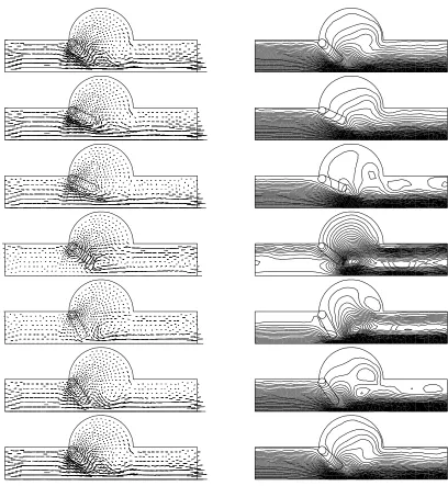
Figure 3. Velocity field and Streamlines at time steps 295–305–310–320–335–340–345
References
[1] http://www.freefem.org, source code : http://www.freefem.org/examples/NSpenal.edp.
[3] R. Glowinski, T.W. Pan, T.I. Hesla, D.D. Joseph, A distributed lagrange multiplier/fictitious domain method for particulate flowInt. J. of multiphase flow25, 1998, pp. 755-794.
[4] H.H. Hu,Direct simulation of flows of solid-liquid mixturesInt. J. of Multiphase flow22, 1996, pp. 335-352.
[5] A. A. Johnson, T. E. Tezduyar,Simulation of Multiple Spheres Falling in a Liquid-Filled TubeComputer Methods in Applied Mechanics and Engineering134, pp. 351-373, 1996.
[6] B. Maury,Optimisation sous Contrainte et M´ethode des ´El´ements Finis, Notes de Cours. Universit´e Paris-Sud (2005). [7] B. Maury,Direct simulations of 2D fluid-particle flows in biperiodic domainsJournal of computational physics156, 1999, pp.
325-351.
[8] O.A. Oleinik, A.S. Shamaev, and G.A. Yosifian, Mathematical Problems in Elasticity and Homogenization North-Holland, Amsterdam, 1992.
[9] T.N. Randrianarivelo, G. Pianet, S. Vincent, J.P. Caltagirone, Numerical modelling of solid particle motion using a new penalty method, Int. J. Numer. Meth. Fluids 2005,47, 1245-1251.