Multi-frequency piezomagnetoelastic energy harvesting in the monostable mode

Journal of Theoretical and Applied Vibration and Acoustics 4(1) 1-18 (2018)

I S A V

Journal of Theoretical and Applied

Vibration and Acoustics

journal homepage: http://tava.isav.ir

Multi-frequency piezomagnetoelastic energy harvesting in the

monostable mode

Amin Yousefpour

, Arash Bahrami

, Mohammad Reza Haeri Yazdi

a _{MSc. Student, School of Mechanical Engineering, University of Tehran, Tehran, Iran.}

b _{Assistant professor, School of Mechanical Engineering, University of Tehran, Tehran, Iran}

c _{Professor, School of Mechanical Engineering, University of Tehran, Tehran, Iran}

A R T I C L E I N F O A B S T R A C T

Article history:

Received 8 March 2018

Received in revised form 28 April 2018

Accepted 30 April 2018

Available online 19 May 2018

The present article investigates effects of the multi-frequency excitation on the output power of a piezomagnetoelastic energy harvester. The piezomagnetoelastic power generator is assumed to operate in themono-stable mode. A perturbation technique based on the method of multiple scales is employed to develop an analytical solution to nonlinear differential equations governing the system dynamics. In addition, a Runge-Kutta numerical scheme is used to solve the differential equations. It is shown that the perturbation solution is in a close agreement with the numerical solution. The system response is determined for several cases including super-harmonic, combination and simultaneous resonances. The steady-state output voltage is then obtained for each case and compared with that of a single-frequency excitation. Due to nonlinearities present in the system, a multi-frequency excitation gives rise to complicated phenomena such as combination and simultaneous resonances. It is found out that exploiting these resonances can significantly increase the amount of energy harvested.

© 2018 Iranian Society of Acoustics and Vibration, All rights reserved. Keywords:

Energy harvesting

Multi-frequency excitation

Method of multiple scales

Piezomagnetoelastic

1. Introduction

Human's life has historically depended on using ambient energy to fulfil the essential energy needs such as ambient energy employed in sailing ships, waterwheels and windmills. While our life still relies on such techniques to provide a portion of the ever-increasing demand for energy, the rapid change in technological trends requires modifying or even revolutionizing these old [1-3] concepts.

* _{Corresponding author:}

E-mail address:arash.bahrami@ut.ac.ir(A. Bahrami)

2 Energy harvesting is the act of scavenging ambient energy available in the environment and transforming it into a usable form. Vibrational energy harvesters are one of the most common types of energy harvesters. The energy harvested from ambient vibrations is sufficient to provide the power required for low-power devices such as data transmitters, wireless sensors, medical implants, and controllers. This way, technical issues like wiring complications is reduced and in some applications the frequent need of changing batteries is removed [4, 5].

Several mechanisms have been utilized so far, to convert vibrational energy into electricity such as piezoelectric materials, electromagnetic and electrostatic mechanisms [6, 7]. Piezoelectric energy harvesters are the most common devices already used to obtain electrical energy from ambient, especially when dealing with low-frequency ambient vibrations. Consequently, piezoelectric transducers have received considerable attention [8-10]. The most common structure for a vibrational energy harvester is a mechanism consisting of a cantilever beam with piezoelectric patches, attached near its clamped end. External environmental excitations applied at the cantilever base result in large strains near the clamped end, leading to a voltage difference across the piezoelectric patches. The voltage difference may be used to generate a current with a suitable circuit design. This way, mechanical energy of the environment is converted into electrical energy [11, 12]. During the past two decades, many researches have employed piezoelectric energy harvesting in different applications spanning from biomedical devices to microelectromechanical systems. Both experimental and theoretical results have demonstrated that some piezoelectric energy harvesters are capable of harvesting energy from various locations of human limbs (wrist, thigh, and ankle) [13]. MEMS-based energy harvesting is the process by which ambient energy has gathered and converted into electricity, employed in small autonomous devices. This energy harvester is used for low-power electronic devices [14].

3 and nonlinear MEMS harvesters to recharge the batteries of the pacemakers by scavenging the vibrational energy from the heartbeats. They suggested piezomagnetoelastic configuration to rise the frequency bandwidth of the energy harvesting system and to decrease its sensitivity to heart rate. They proposed the configuration, illustrated in Fig. 1 for the monostable energy harvesting. The beam is a bimorph, made in micro scale. In this system, the nonlinear behavior is caused by the applied magnetic forces.

Fig.1: The nonlinear energy harvesting configuration [18].

Erturk and Inman [19] have investigated the piezomagnetoelastic energy harvester in the monostable mode and used the method of multiple scales to determine the response of the system at the primary resonance. Stanton et al.[20] have employed the method of harmonic balance to study the response stability and effect of parameter variations on the output power at the primary resonance. Karami and Inman [21] have used a perturbation method to study small-amplitude oscillations of the system near its stable equilibrium points. All these studies have focused on a single-frequency excitation around the system fundamental frequency.

Abdelkefi et al.[22] have considered the multi-frequency excitation to enrich the level of energy, harvested from a piezoelectric cantilever subjected to a combination of bending and torsional loads. They have considered the excitation as the sum of three harmonic terms. Cantilever first three natural frequencies are tuned to excitation frequencies by adjusting the asymmetry of tip masses. They have performed a parametric study to determine the advantages of tuning the structure to harvest energy at multi-frequency excitation. Foisal et al.[23] have studied an array of four generators and showed the possibility of harvesting energy from different environmental frequencies for this system. They used the magnetic spring technique as a cantilever to scavenge energy from vibrations.

4 resonance and RMS† _{values of the output voltage are determined for each case. A Runge-Kutta} scheme is then employed to verify the results obtained based on the method of multiple scales. It is observed that the perturbation solution is in a close agreement with the numerical solution.

Fig. 2: Piezomagnetoelastic power generator [19]

2. Mathematical model

Fig. 2 presents a schematic of the beam with piezoelectric layers and its electrical circuit. This structureconsists of a steel beam and two bonded piezoelectric layers. Piezoelectric layersharvest energy from the beam deflections. Applied magnetic forces in this system induce the nonlinear behaviour. The governing equations for a beam with a magnet on its tip, oscillating between two permanent magnets located symmetrically near the free end were derived by Moon and Holmes in 1979 [17]. In the present research, we consider the same model with two harmonic external excitations.

The non-dimensional governing equations of a monostable piezoelectric energy harvester with a cubic nonlinearity under a multi-frequency excitation is given by[19] :

2 3

0 0 1 1 2 2

2

2 cos(

) 2

cos(

)

x



 

x





x





x





v



f



t



f



t





0

v







v





x





where x is dimensionless cantilever tip deflection, t is dimensionless time, v is dimensionless output voltage, ω0 is the first natural frequency of the system, is the coefficient of the cubic nonlinear term, f1 is dimensionless excitation amplitude at frequency Ω and f2 is dimensionless excitation amplitude at frequency Ω , λ is the reciprocal of the dimensionless time constant of the

5 resistive–capacitive circuit (it is inversely proportional to the load resistance) and χ is dimensionless piezoelectric coupling term in the mechanical equation. In addition, κ denotes dimensionless piezoelectric coupling term in the electrical equation, and a dot signifies differentiation with respect to time. Furthermore, ε is a small bookkeeping parameter and µ is a mechanical damping term[19].

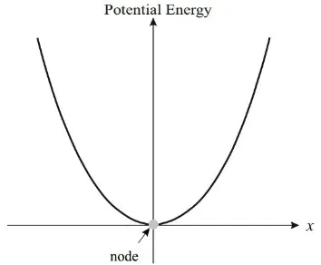
In this research, we investigate a system with only one equilibrium point (monostable mode). The cantilever is assumed to oscillate around its equilibrium position (i.e., zero-deflection position). Fig. 3 shows the potential energy function for the monostable mode, demonstrating that the system has a single equilibrium point.

Fig. 3: Potential energy function for monostable mode.

To determine the tip deflection and the output voltage, Eqs. (1) and (2) should be solved either analytically or numerically. The main advantage of analytical methods such as the method of multiple scales compared to numerical methods such as Runge-Kutta is that the method of multiple scales is able to determine where superharmonic, combination and simultaneous resonances occur. It is really difficult to predict these secondary resonances using numerical methods like Runge-Kutta. In addition, we can obtain a closed-form expression for the frequency-response function based on the perturbation method. Having this closed-form expression, we can change different parameters such as excitation frequency and excitation amplitude and investigate the effect of each parameter on the system behaviour. Moreover, the method of multiple scales captures unstable branches of the frequency-response curve which require backward integration and are generally very hard to obtain numerically.

The method of multiple scales is used in this section to solve equations governing the system dynamics. For small nonlinearities, the solution may be expanded in terms of powers of ε:

2

0

( , )

( , )

(

)

x



x T T





x T T



O



2

0

( , )

( , )

(

)

6 Where the Tn = εn _{(n = 1, 2) represent different time scales. To render this expansion uniformly} valid, we use the method of multiple scales [24]. In terms of the new time scales Tn, the time derivatives are written as:

0 1

d

D

D

dt







(5)

2

2 2 2

0 0 1 1 0

2

2

(

2

)

d

D

D D

D

D

dt













(6) Where n n D T   

. Substituting Eqs. (3) and (4) into Eqs. (5) and (6), and the subsequent results into Eqs. (1) and (2) yields the following differential equations for different powers of ε:

0

:



2 2

0 0 0 0

2

cos(

)

2

cos(

)

D x





x



f



t



f



t

0 0 0 0 0

D v





v

 



D x

1

:



2 2 3

0 1 0 1

2

2

D x





x

 

D D x





D x





x





v

0 1 1 1 0

(

)

D v





v

 

D v





D x



D x

The general solutions to Eqs. (7) and (8) are given by:

0 0 1 0 2 0

0 1 1 2

i T i T i T

x



A e



F e



F e



cc

0 0 1 2 0 0

1 1 1 2 2

0 2

1 2

i T i T i T T

A i F i F i

v e e e A e cc

i i i

 















where cc is the complex conjugate of the preceding term. Moreover, 1 1 2 2

0 1 f F     and 2

2 2 2

0 2 f F     .

7 0 0

1 0 2 0

0 0 1 0 2 0 0 1 0

2 2 2 2

0 1 0 1 0 1 0 1 1 1 1 2 1

2 2 2 2

1 0 1 1 1 2 1 2 0 1 1 1 2 2

3 3 3 (2 ) (2

3 3 3 2 2

1 1 2 1 1 1 2

[2 ( ) 3 ( 2 2 ) ]

[2 3 (2 2 )] [2 3 (2 2 )]

3 3

i T

i T i T

i T i T i T i T i

D x x i A A A A F F A e

i A A F F F e i A A F F F e

A e F e F e A F e A F e

                                       

     0 2 0 0 1 0

0 2 0 0 1 0 0 2 0 0 1 0 0 2 0

0 1 2 0 0 1 2 0 0 1 2 0

) 2 (2 ) 1 1

( 2 ) ( 2 ) ( 2 ) ( 2 ) ( 2 )

2 2 2 2 2

1 2 1 1 1 2 1 1 1 2

( ) ( ) ( )

1 1 2 1 1 2 1 1 2

3

3 3 3 3 3

6 6 6 6

T i T

i T i T i T i T i T

i T i T i T

A F e

A F e A F e A F e A F e A F e

A F F e A F F e A F F e A

                                         

    0 1 2 0

1 2 0 1 2 0 1 2 0 2 1 0 0 0

2 0 1

( ) 1 1 2

(2 ) ( 2 ) ( 2 ) (2 )

2 2 2 2 1

1 2 1 2 1 2 1 2

1 1 2 2

1 2

3 3 3 3

i T

i T i T i T i T i T

i T i T

F F e A i

F F e F F e F F e F F e e

i F i F i

e e i i                                        (13)

The complex conjugate of is represented by . Coefficients A1, appearing in Eqs. (11) and (12) are obtained by eliminating so called troublesome terms (including secular and small-divisor terms) in Eq. (13) (reference[24] may be consulted for more details).

3. Results and discussion

The mechanical and electrical properties of the system considered here are presented in table 1.[19] In this investigation, the effect of different excitation frequencies is studied on the system behavior and the output power. Numerical simulations are presented based on the perturbation solution for several cases including superharmonic, combination and simultaneous resonances.

Table 1. Parameters of the reference model

µ = 0.01 α =0.05

χ = 0.05 λ = 0.05

κ = 0.5 ω0 = 1

3.1.Superharmonic resonance

For the superharmonic resonance, the external excitation is assumed to be close to one-third of the first natural frequency of the system Ω1 ω0 . The proximity of Ω1 to ω0 is expressed by introducing the detuning parameter



1 0

3

 







8

1 0 0 0 0 0 0 0 0 1

3



T



(







)

T





T





T





T





T

The modulation equation is obtained by eliminating the secular and small-divisor terms in Eq. (13):

1

2 2 1 3

0 1 0 1 1 1 1 2 1 1

2

i

(

A

A

) 3 (

A A

2

F

2

F A

)

Ai

F e

0

i













 















Letting ₁ 1

2

i

A  a ein Eq. (16) and separating real and imaginary parts of the modulation equation, following equations are found:

2 3

0 2 1

sin(

)

2(1

)

a

a

 

a

 



F



T





  









(17-a)

2 2 2 3

0 1 2 2 1 1

1

1

3 (

2

2

)

cos(

)

4

2

2(1

)

a

a

a

F

F

a



F

T

 











 













(17-b)

Eqs. (17-a) and (17-b) are made autonomous by introducing:

1

T











The steady-state motions correspond to a 0. For steady-state oscillations, the frequency response equation is obtained as:

2 3 2

2 2 2 1 2

1 2 2 2 0 2

0

( )

1 1 1

3 ( 2 2 )

4 2 2(1 ) 2(1 )

F a F F

a            _{ }         _  _   _  _    (19)

Equation (19) expresses the frequency response equation associated with the superharmonic resonance for the monostable energy harvesting system.

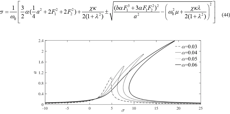
9 Fig. 4 shows the frequency-response curves (a vs. ) associated with the homogeneous part of the response at superharmonic resonance with different nonlinear coefficients. The value of homogeneous response amplitude increases near superharmonic resonance (the response amplitude is equal to 0.184 for  0.05 and 2). Also, it is seen that the response amplitude increases by increasing the nonlinear coefficient of the system. Therefore, the energy extracted increases with the coefficient of the nonlinear term. It should be noted that the increasing this coefficient is limited by physical constraints and depends on the geometry and physical features of the system. In fact, after a certain value the harvester operational mode changes and so do the governing equations. The value of depends on the magnetic potential, the stiffness coefficient of the system and the beam thickness. According to references[19, 24], value of can vary between 0 (for the linear system) and 0.158 for the monostable mode. In this study, we have considered that varies from 0.03 to 0.06.

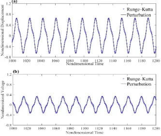
As expected, the harvester exhibits hardening behavior for positive values of the nonlinear coefficient. Time histories for the tip displacement and the harvested electrical voltage are illustrated in Fig. 5 at superhamonic resonance with Ω1 ω0 , Ω2=0, f1 = 0.5 and f2 = 0 For this case, the output voltage RMS value is 0.1998. We note that results of numerical solution and those obtained based on the method of multiple scales are compared in this Figure. As seen in the Fig.5, the results are in excellent agreement.

10

3.2.Combination resonance

Now, we consider that excitation is composed of two harmonic terms:

1

cos(

)

cos(

)

f



t



f



t

Because of the cubic nonlinearity appearing in Eq. (1), combination resonances occur for particular values of the excitation frequencies; that are:

0

2



    

And

0

1

(

)

2





  

where p =1 and 2 and q =1 and 2. Among all possible external excitations satisfying Eqs. (21) or (22), we choose the following case for the numerical simulation: Ω1 ω0 and Ω2 ω0 and assume

2

2





   



with being the detuning parameter. Using equation (23),

(

  

2 )

T

2 1 0 0 0 0 0 0 0 0 1

(

  

2

)

T



(







)

T





T





T





T





T

Substituting Eq. (24) into Eq. (13) and eliminating troublesome terms (secular terms and small-divisor terms) in Eq. (13) yield the modulation equation for the combination resonance as:

1

2 2 1 2

0 1 0 1 1 1 1 2 1 1 2

2

i

(

A

A

) 3 (

A A

2

F

2

F

)

A

A i

3

F F e

0

i















 















Next, we let 1

1

2

i

A



ae

2 2 2

2 2 2 1 2 2

1 2 2 2 0 2

0

(3 )

1 1 1

3 ( 2 2 )

4 2 2(1 ) 2(1 )

F F

a F F

a



 

   

  

 

 

 

     _  _

  _  _ 

 

11

Fig. 6: Frequency response at the combination resonance (Ω ≈ , Ω ≈ ) for the monostable mode with different nonlinear stiffness coefficients

Fig. 6 presents the frequency response corresponding to homogeneous part of the response at the combination resonance for the monostable mode with different nonlinear coefficients. It is observed that the combination resonance results in a considerable increase in the response amplitude. The value of the response amplitude increases near the combination resonance leading to enhance energy harvester performance. The response amplitude is equal to 0.54 for 0.05 and 4. Moreover, it is seen that the maximum amplitude increases by increasing the nonlinear stiffness coefficient. Therefore, the energy harvested in this case increases with the coefficient of the nonlinear term.

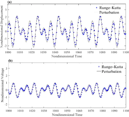
The displacement and the output voltage are depicted versus time in Fig. 7 for combination resonance with Ω1 ω0 , Ω2 ω0, f1 = 0.5 and f2 = 0.5 . Both numerical and perturbation solutions are employed to plot Fig. 5. It is found out that the perturbation solution is capable of accurate prediction of the steady-state response. It is noted that when the beam is excited through two frequencies Ω ≈ and Ω ≈ separately, the equivalent RMS value for the output voltage is 0.2553. By applying two excitations at the same time, the combination resonance occurs and the RMS value of the output voltage is found to be 0.2986.

3.3.Simultaneous resonance

When the system is excited with a multi-frequency excitation, depending on the value of excitation frequencies and fundamental frequency of the system more than one resonance might occur simultaneously. For instance, both subharmonic and superharmonic resonances can occur simultaneously or both superharmonic and combination resonances may occur simultaneously [16] . For a two-frequency excitation, secondary resonances that may take place are:

0

3

or

3



 



 

0 1 0 2

1 1

3 or 3

12

0 2 2 1 or 0 2 1 2





0

2



   

A close examination of Eqs. (27) through (30) reveals that the only possible simultaneous resonances are:

2

9

3



   

2 1

3



   

2 1 0

1

3



   

2 1 0

5

5

3



   

13

2 1 0

7

7

3



   

2 1 0

2

2

3



   

2 1 0

7

7

3



 

 

2 1 0

5

5

3



   

(38)

The case of simultaneous resonance given by Eq. (36) in which the superharmonic resonance and a combination resonance occur simultaneously is considered here for numerical simulations. To investigate this case, two detuning parameters 1_and 2 _{are introduced as:}

2 0 1

3

2

 







(39-a)

1 0 2

3

 







Then, _{1 0}T and _{2 0}Tare rewritten in the following form:

1 0 0 1 0 0 0 1 1

1

1

1

(

)

3

3

3

T





T



T



T











2 0 0 0 1 0 0 0 2 1

2 2 2 2

3 3 3 3

T T T T  T

     (40-b)

The modulation equation is determined by starting from Eq. (13) and employing the same procedure, performed for combination resonance to eliminate troublesome terms:

2 1 1 1 1

4 1

( )

2 2 1 3 2 3 3

0 1 0 1 1 1 1 2 1 1 1 2

2i (A A) 3 (A A 2F 2F )A A i F ei T 3 F F ei T 0

i                      (41)

Introducing the polar form ₁ 1

2

i

A _ ae _{and substituting it into in Eq. (41) result in the following}

equations:

2 3 2

0 2 1 1 1 1 2 2 1 1

4 1

sin( ) 3 sin(( ) )

2(1 ) 3 3

a

a  a   F T  F F   T  

        



14

2 2 2 3 2

0 1 2 2 1 1 1 1 2 2 1 1

3 1 4 1

( 2 2 ) cos( ) 3 cos(( ) )

2 4 2(1 ) 3 3

a

a  a a F F  F T  F F   T  

         



(42-b)

The steady-state motion exists if and only if both _{1 1}T  and (4 ₂ 1 ₁) ₁

3 3 T are constant which

implies:

1 2











Substituting Eq. (43) into equation (42-a) and (42-b), the following frequency-response equation is determined for the steady-state response:

2

3 2 2

2 2 2 1 1 2 2

1 2 2 2 0 2

0

( 3 )

1 3 1

( 2 2 )

2 4 2(1 ) 2(1 )

b F F F

a F F

a

 

 

   

  

 

 



 

     _  _

  _  _ 

 

(44)

Fig. 8: Frequency response at the simultaneous resonance (Ω ≈ , Ω ≈ ) for the monostable mode with different nonlinear stiffness coefficients

15

Fig. 9:Time history for the simultaneous resonance (Ω1  ω0 and Ω2  ω0): (a) displacement and (b) voltage

Fig. 9 presents time histories of the displacement and the harvested voltage for simultaneous resonance when Ω1 ω0 and Ω2 ω0. For this case, excitation amplitudes are assumed to be f1 = 0.5 and f2 = 0.5. The RMS voltage is equal to 0.5137 which is 2.57 times the voltage harvested at the superharmonic resonance (Ω1 ω0 ).

16

Table 2:Normalized output voltage Case studies Normalized

RMS voltage (perturbation)

Normalized RMS voltage (Runge–Kutta)

Normalized maximum voltage (perturbation)

Normalized maximum voltage (Runge–Kutta) Superharmonic resonance

Ω1  ω0

0.1998 0.1975 0.3276 0.3283

Combination resonance

Ω1  ω0, Ω2 ω0 0.2986 0.2951 0.6140 0.5580

Simultaneous resonance

Ω1  ω0 , Ω2  ω0 0.5137 0.5082 1.0071 0.9364

Using parameters given by references [19] and [25], the actual harvested voltage and maximum power are obtained for each case. Table 3 shows the amount of actual voltage and power for superharmonic, combination and simultaneous resonances.

Table 3: Actual output voltage with perturbation method

Case studies RMS voltage(V) Maximum voltage(V) Maximum power(mW) Superharmonic resonance

Ω1  ω0 3.5404 5.8050 3.3698

Combination resonance

Ω1  ω0, Ω2 ω0 5.2912 10.8800 11.8374

Simultaneous resonance Ω1  ω0 , Ω2  ω0

9.1027 17.8458 31.8472

4. Conclusions

17 for a rather wide range of the frequency band. Therefore, more amount of energy is harvested. Numerical studies conducted throughout the paper show that under similar conditions, a higher amount of energy is harvested in a multi-frequency excitation rather than a single-frequency excitation. In addition, it is found out that simultaneous and combinations resonances generate more power compared to the superharmonic resonance.

References

[1] H.A. Sodano, G. Park, D.J. Inman, Estimation of electric charge output for piezoelectric energy harvesting, Strain, 40 (2004) 49-58.

[2] G.K. Ottman, H.F. Hofmann, A.C. Bhatt, G.A. Lesieutre, Adaptive piezoelectric energy harvesting circuit for wireless remote power supply, IEEE Transactions on power electronics, 17 (2002) 669-676.

[3] S. Jiang, X. Li, S. Guo, Y. Hu, J. Yang, Q. Jiang, Performance of a piezoelectric bimorph for scavenging vibration energy, Smart Materials and Structures, 14 (2005) 769.

[4] S. Roundy, P.K. Wright, A piezoelectric vibration based generator for wireless electronics, Smart Materials and structures, 13 (2004) 1131.

[5] M.A. Karami, D.J. Inman, Equivalent damping and frequency change for linear and nonlinear hybrid vibrational energy harvesting systems, Journal of Sound and Vibration, 330 (2011) 5583-5597.

[6] S. Priya, D.J. Inman, Energy harvesting technologies, Springer, 2009.

[7] D. Guyomar, A. Badel, E. Lefeuvre, C. Richard, Toward energy harvesting using active materials and conversion improvement by nonlinear processing, IEEE transactions on ultrasonics, ferroelectrics, and frequency control, 52 (2005) 584-595.

[8] S.R. Anton, H.A. Sodano, A review of power harvesting using piezoelectric materials (2003–2006), Smart materials and Structures, 16 (2007) R1.

[9] S.P. Beeby, M.J. Tudor, N.M. White, Energy harvesting vibration sources for microsystems applications, Measurement science and technology, 17 (2006) R175.

[10] K.A. Cook-Chennault, N. Thambi, A.M. Sastry, Powering MEMS portable devices—a review of non-regenerative and non-regenerative power supply systems with special emphasis on piezoelectric energy harvesting systems, Smart Materials and Structures, 17 (2008) 043001.

[11] M.F. Daqaq, R. Masana, A. Erturk, D.D. Quinn, On the role of nonlinearities in vibratory energy harvesting: a critical review and discussion, Applied Mechanics Reviews, 66 (2014) 040801.

[12] A. Erturk, J. Hoffmann, D.J. Inman, A piezomagnetoelastic structure for broadband vibration energy harvesting, Applied Physics Letters, 94 (2009) 254102.

[13] K. Fan, B. Yu, L. Tang, Scavenging energy from human limb motions, in: Active and Passive Smart Structures and Integrated Systems 2017, International Society for Optics and Photonics, 2017, pp. 101642P.

[14] Y. Luo, R. Gan, S. Wan, R. Xu, H. Zhou, Design and analysis of a MEMS-based bifurcate-shape piezoelectric energy harvester, Aip Advances, 6 (2016) 045319.

[15] S.C. Stanton, A. Erturk, B.P. Mann, D.J. Inman, Resonant manifestation of intrinsic nonlinearity within electroelastic micropower generators, Applied Physics Letters, 97 (2010) 254101.

[16] A.H. Nayfeh, D.T. Mook, Nonlinear oscillations, John Wiley & Sons, 2008.

[17] F.C. Moon, P.J. Holmes, A magnetoelastic strange attractor, Journal of Sound and Vibration, 65 (1979) 275-296. [18] M. Amin Karami, D.J. Inman, Powering pacemakers from heartbeat vibrations using linear and nonlinear energy harvesters, Applied Physics Letters, 100 (2012) 042901.

[19] A. Erturk, D.J. Inman, Piezoelectric energy harvesting, John Wiley & Sons, 2011.

[20] S.C. Stanton, B.A.M. Owens, B.P. Mann, Harmonic balance analysis of the bistable piezoelectric inertial generator, Journal of Sound and Vibration, 331 (2012) 3617-3627.

[21] M.A. Karami, P.S. Varoto, D.J. Inman, Analytical Approximation and Experimental Study of Bi-Stable Hybrid Nonlinear Energy Harvesting System, in: ASME 2011 International Design Engineering Technical Conferences and Computers and Information in Engineering Conference, American Society of Mechanical Engineers, 2011, pp. 265-271.

[22] A. Abdelkefi, A.H. Nayfeh, M.R. Hajj, F. Najar, Energy harvesting from a multifrequency response of a tuned bending–torsion system, Smart Materials and Structures, 21 (2012) 075029.

18

[24] A.H. Nayfeh, Introduction to perturbation techniques, John Wiley & Sons, 2011.