Please cite this article as: M. I. Khodakarami, H. R. Khalaj Hedayati, Application of Decoupled Scaled Boundary Finite Element Method to Solve Eigenvalue Helmholtz Problems, International Journal of Engineering (IJE), IJE TRANSACTIONS B: Applications Vol. 33, No. 2, (February 2020) 198-204
International Journal of Engineering
J o u r n a l H o m e p a g e : w w w . i j e . i rApplication of Decoupled Scaled Boundary Finite Element Method to Solve
Eigenvalue Helmholtz Problems
M. I. Khodakarami*, H. R. Khalaj Hedayati
Faculty of Civil Engineering, University of Semnan, Semnan, Iran
P A P E R I N F O
Paper history:
Received 9 March 2019
Received in revised form 9 November 2019 Accepted 16 Januray 2020
Keywords:
Macro Element Helmholtz Equation Eigenvalue Analysis
Decoupled Scaled Boundary Finite Element
A B S T R A C T
A novel element with arbitrary domain shape by using decoupled scaled boundary finite element (DSBFEM) is proposed for eigenvalue analysis of 2D vibrating rods with different boundary conditions. Within the proposed element scheme, the mode shapes of vibrating rods with variable boundary conditions are modelled and results are plotted. All possible conditions for the rods ends are incorporated in analysis. The considered element stiffness and mass matrix are developed and extracrted. This element is able to model any curved or sharp edges without any aproximation and also the element is able to model any arbitrary domain shape as a single element without any meshing. The coefficient matrices for the element such as mass and stiffness matrices are diagonal symmetric and all equations are decoupled by using Gauss-Lobatto-Legendre (G.L.L) quadrature. The element is used in order to calculate modal parameters by Finite element method for some benchmark examples and comparing the answers with Helmholtz equation solution. The most important achievment of this element is solving matrix equations instead of differential equations where cause faster calculations speed. The boundaries for this element are solved with matrix calculation and the whole interior domain with solving governing equations numerically wich leads us to an exact answer in whole domain. The introduced element is applied to calculate some benchmark example which have exact solution. The results shows accuracy and high speed of calculation for this method in comparison with other common methods.
doi: 10.5829/ije.2020.33.02b.03
NOMENCLATURE
0
D Coefficient matrix LCO Local Coordinate Origin
1
D Coefficient matrix Greek Symbols
F Load vector Density (kg/m3)
M Mass matrix Tangentical coordinate
u
Displacement
Radial coordinateu First derivative of displacement Natural frequency relation function
u Second derivative of displacement
Natural frequency1. INTRODUCTION1
In early numerical methods there were only two alternative solution procedures available to solve a problem [1]. Either internal cells had to be defined or
*Corresponding Author Email: [email protected] (M. I. Khodakarami)
fundamental solution had to be found which took into account all the terms in the governing equation [1-3]. After improvement of the numerical methods in recent decades some new methods were added to this type of analysis, any of these methods have advantageous and disadvantages [4, 5]. As an engineer it is very important to select a method with high speed of calculation and high accuracy of answers. In this way mesh-less
methods were developed and used widely in order to solve problems with high speed of calculation but the accuracy of answer was always an important factor for designers and engineers [6-8]. The most widely used procedure in solid mechanics and many other fields of engineering and physics are the finite element method (FEM) and the boundary element method (BEM). The unknown continuous solution is replaced, for instance in statics, by algebratic equations in terms of parameter definig the approximate solution. Both methods exhibit their specific features, advantages and disadvantages. In the FEM the domain is spatially dicretised into non-overlapping elements. In each such finite element, shape functions in the form of polynomials interpolate, for instance, the displacements. Standard numerical integration of these regular functions leads to a simple approximation for the behaviour of each finite element, for instance, consisting of the (symmetric) static stiffness and mass matrices [5]. In the BEM, only the boundary is discretised spatially into elements, leading to a reduction of the spatial dimension by one. This diminishes the effort of data prepration and leads to fewer unknowns. However, a so-called fundamental solution, satisfying the governing differential equations in the domain must be available in literature [9, 10]. By combinig the advantages of the BEM and FEM the scaled boundary finite element method (SBFEM) were created and used in order to solve many semi analytical problems [11]. The method is a semi-analytical procedure for solving linear partial differential equations.
A modification of the scaled boundary finite element method with diagonal coefficient matrices (DSBFEM) has been proposed for solving potential problems and it is applied to solve easto-estatic and elasto-dynamic problems [12-14]. In this study, we used decoupled scaled boundary finite element method (DSBFEM) as an element in analysis with FEM procedure for eigenvalue Helmholtz problems and benchmark examples with availavle exact solutions.
The Lagrange polynomials is used as mapping functions and also Gauss-Lobatto-Legendre quadrature is employed in order to calculate coefficient matrices.
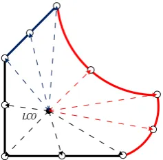
LCO
Figure 1. Ability of suggested technique in modelling of
The technique is used to solve 2D problems [15]. One of the most important achievment of this technique is the ability of using it to model arbitrary shape problem domains as a single element without any division to subset elements or meshing the domain (Figure 1). By this way the Local Coordinate Origin (LCO) which was at a point with direct view to whole domain, is relocated at center of area of problem which helps us to obtain many arbitrary problem shapes as a unique domain to solve the problem. The proposed element’s relocated LCO causes changes in tangential and radial equations. The element’s boundary nodes equations remain decoupled as we use GLL quadrators. Mass and stiffness matrices creations need to make new formulas and using new methods which described in following scopes of this paper. The formulas were developed and some benchmark examples are solved by these techniques and results are plotted and compared with exact solution.
2. A REVIEW ON DSBFEM
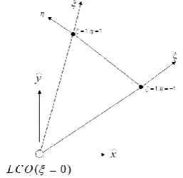
The basic concepts of DSBFEM is expressed in literature [14]. The novelty of this paper is considering whole domain as a single element in FEM analysis approach by relocating local-coordinate-origin (LCO) from a corner of the domain with direct view to whole boundary to center of the area of element which can cause to calculate huge elements with arbitrary shapes without meshing and subset elements. The global Cartesian coordinates in 2D problems are , in which using the Lagrange polynomials would be transmitted into local coordinates , where is
radial coordinate from the LCO to the
boundaries and is tangential coordinate which varies between -1 and +1 on the boundaries (Figure 2.). Each element on the boundaries is analogous to a line, the geometry of a boundary point can be transferred to radial tangential coordinates by using higher order of Chebyshev polynomials mapping function. After calculating stiffness and mass matrix by this method, modal analysis is possible and natural frequencies, periods and mode shapes are available by solving main
dynamical equation of modal analysis .
The stiffness and mass matrices for the presented element can be calculate by using new techniques which are described in this paper and are presented in the following scopes.
Mass matrix in this method is similar to DSBFEM and fully described in literature [14], the novelty is calculating the stiffness matrix for the presented element which described in following scopes.
Figure 2. Radial , Tangential coordinates
local-coordinate-origin (LCO) is selected at center of the area of element which can cause to calculate huge elements with arbitrary shapes. The general formulation of transfer operators and mapping functions are described in literature [16]. By considering transform equations, the Lagrange polynomials have the properties of the Kronecker delta at any control point . As it is clear to prepare parent element, nodes are required, where two end-nodes are located at the extremity of the element and other remained nodes are located at Gauss-Lobbato-Legendre points. These points are the first roots of the first order derivative of order Legendre polynomials:
( ) 0
n
d P
d = (1)
All formulation of DSBFEM is reliable in the element; so the governing equation for engineering problems is solved by the rules of DSBFEM for 2D problems:
( )
( )
( )
0 1
, ,
1
. . b [ ]{ }
ii i ii i i
D u D u F M u
+ + = (2)
The coefficient matrices of Equation (2) is completely extracted and described in literature [16]. The mentioned coefficient matrices are also use in proposed element as well and use in order to create stiffness and mass matrix for the element which leads us to extract Stiffness and Mass matrices for whole domain. It is worth noting that the coefficient matrices in Equation (2) can be non-zero or in some circumstanses they can be zero which depends on the boundary shapes.
2. 2. Modal Analysis with Suggested Element In order to calculate modal parameters for a problem, general formulation of structural dynamic can be
applied . While we have relocated the
LCO, we have to calculate stiffness matrix by considering new condition.
3. MATHEMATICAL DEVELOPMENT OF THE SUGGESTED ELEMENT
As mentioned above, by relocating LCO we have to calculate stiffness matrix and mass matrix for suggested technique. In following scopes, the formulation for new introduced element is described and formulation is developed.
3. 1.Stiffness Matrix Creation To create the stiffness matrix for an element, consider each node on boundaries is connected to the LCO by a line which has the properties of the whole domain. This lines are connected together at LCO. All this lines have their own stiffness in their local coordinates let us call these lines sub-elements. Each line of stiffness matrix is made of applying a unit displacement at any degree of freedom and calculate the reaction of other degrees of freedom. This procedure needs to be calculated in two main steps:
• First: Fixing all degrees of freedom except one we want to apply a unit displacement and calculate the respectively force which made by the unit displacement at intersection point of the sub-elements (LCO).
• Second: Divide the calculated force at LCO between all the sub-elements respecting to their stiffness.
3. 1. 1. Applying Unit Displacement The sub-elements in their nature can be assumed as a bar element and since we are calculating at 2D space, each node has two degrees of freedom while we regardless the flexural freedoms. LCO can be considered as a restrain for each sub-element. It is clear that this restrain is not rigid and also one can find out that the rigidity of LCO is consist of rigidity of all incoming sub-elements. The produced force due to displacement of a node at local coordinate can be calculated as Equation (3)
0
i
F =D u (3)
when each degree of freedom is released to move freely in case of non-exist of external forces, the governing differential equation for element is linear in corresponding to :
{ } ( ) { }
u
i
=
A
i
+
{ }
B
i (4)where in Equation (4) the Bi term is displacement at
LCO which is zero in this case and due to boundary conditions at , and Ai term Equation (4) can be 1
corresponding to applied displacement at node.
( )
( )
0, , 0, 1,
i
i
i k u
i k
i k u
i k
=
=
=
=
(5)
If direct boundaries imagine for the domain, only term is non-zero in equations. By considering the LCO as a restrain, its rigidity is made of all arrival sub-elements to the LCO, this rigidity can be calculating by the following formula
0 0
1
n
LCO
i i
D D
=
=
(6)where n is the amount of nodes which considered at the boundaries. The forces which calculated by Equation (8) can make at LCO.
0 1 0
LCO i LCO i i
u =
D − D u (7)3. 1. 2. Returning the LCO Force The produced force at LCO due to applying a unit displacement at a degree of freedom, can be divide between all sub-elements which arrived at LCO. There are two situations can be considered. The first is reflection and the second is refraction. General formula to calculate refracting force to each sub-element can be written as Equation (8)
( )
0
( ) i 0
i i
D u F
− =
(8)
the term can be calculated as follow for k-element
0( ) ( ( ))
i i
LCO k LCO
i i
F
=
D u +
u−u (9)solving Equation (10) leads us to calculate displacement in whole domain among direction as following formula
( )
3
2
1
( )
6 1
2
LCO i i
LCO LCO LCO
u u u
u u u
= −
+ + +
(10)
the stiffness matrix can be created for any sub-element which called i due to release of k sub-element and j is a counter which varies between 1 to n:
(2 1) 0
*(
)
(2 )
. 1
i j
i k k k i
i j
k
k D u
k
−
= = =
(11)
where is defined as follows:
*( )
1 2(
)2 k LCO i
k
u = u − u
(12)
as mentioned above, the term can be calculated as follow
3
14 6
LCO i LCO i
u = u − u − u
(13)
by using equilibrium at LCO, the term can be calculated by Equation (14):
0 1 0
1
1 6 N
LCO LCO j j j
j
u D − D u u
=
= +
(14)Therefore by using achieved amounts in Equation (11), the stiffness matrix will be created after using the formulation for each degree of freedom.
3. 2.Mass Matrix Creation Calculating the mass matrix in this method is similar to DSBFEM and clearly described in literature [16].
4. THE HELMHOLTZ EQUATION
The solution of the Helmholtz equation provides the natural or fundamental frequencies and vibration modes for a system [1, 16-18]. The Equation in its usual form is given by following equation:
2 2
0
u u
+ = (15)
where the coefficient is related to the natural frequency and u represents the displacements. Consider the vibrating rod shown in Figure 3. In this case where and are material properties and is natural frequencies. For illustrating the accuracy of suggested method and comparing with exact solution, some benchmark examples are solved by and compared with the exact solution by Helmholtz equation.
5. NUMERICAL EXAMPLES
This section describes the detailed numerical solution of representative numerical examples in order to illustrate the use of proposed method. Considering the vibrating rod and different boundary conditions leads to calculate modal parameters. Consider the free vibration of the rods shown in Figure 3. The exact solution, natural frequencies and normal mode shapes are given in Table 1. Where and is an integer which takes values up to the order desired.
Figure 3. Vibrating fixed-free rod
TABLE 1. Exact solution of vibrating rods [1]
Type Equation Displacement Con.
Fixed-Free
0
0
. 1 2
n nc
n c l = = −
( )
1
.sin 2 n U x x C n l = − n=1,2,… Fixed-Fixed 0 0 .
n nc
n c l = =
( )
.sin n U x x C n l = n=1,2,… Free-Free 0 0 .n nc
n c l = =
( )
.cos n U x x C n l = n=1,2,…Exact solution for the mentioned rod is shown and compared in Table 2. For clarifying the method’s accuracy, different geometries are considered for the domain with constant and equal to 0.9 in all the examples but width is considered to be 0.2 and 0.4.
5. 2. Free-free Rod As an another example the geometry shown in Figure 3 is considered to be free-free. The results are shown in Table 3. Results is compared with exact solution. It is clear that by increasing boundary nodes the results will be more accurate.
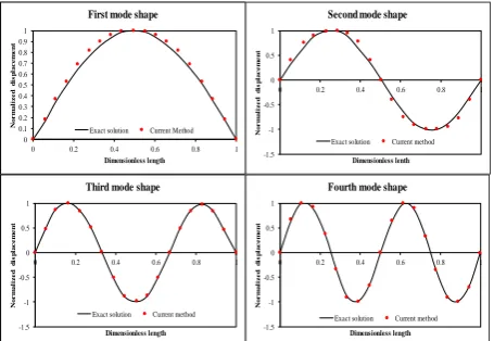
5. 2.Fixed-fixed Rod As an another example the rod geometry which shown in Figure 3 assumed to be both end fixed. The whole domain divided to 32 nodes and results are shown in Table 4. The whole domain is calculated by only 32 boundary nodes and results is compared with exact solution (Figure 5).
TABLE 2. Comparing exact natural frequencies with presented method solution fixed-fixed and 32 nodes element
Mode No.
B=0.2 B=0.4
Exact [1]
Presented
method Err.
Exact [1]
Presented method Err.
1 8.75 8.55 0.02 8.75 8.66 0.01 2 26.25 27.28 0.03 26.25 27.45 0.04 3 43.75 43.3 0.01 43.75 43.89 0.003 4 61.25 60.82 0.007 61.25 75.2 0.22
TABLE 3. Comparing exact natural frequencies with presented method solution free-free and 32nodes element
Mode No.
B=0.2 B=0.4
Exact [1]
Presented method Err.
Exact [1]
Presented method Err.
1 17.854 18.84 0.05 17.584 18.92 0.07 2 35.179 42.62 0.21 35.179 42.71 0.21 3 52.76 52.71 9e-4 52.76 53.24 9e-3 4 67.032 70.12 0.04 67.032 70.53 0.05
TABLE 4. Comparing exact natural frequencies with presented method solution fixed-free rod and 32nodes element
Mode No.
B=0.2 B=0.4
Exact [1]
Presented method Err.
Exact [1]
Presented method Err.
1 17.854 18.84 0.05 17.584 18.92 0.07 2 35.179 42.62 0.21 35.179 42.71 0.21 3 52.76 52.71 9e-4 52.76 53.24 9e-3 4 67.032 70.12 0.04 67.032 70.53 0.05
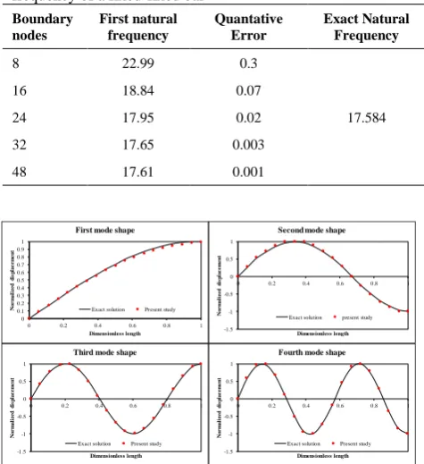
TABLE 5. Effects of increasing boundary nodes to fist natural frequency of a fixed-fixed bar
Boundary nodes First natural frequency Quantative Error Exact Natural Frequency
8 22.99 0.3
17.584
16 18.84 0.07
24 17.95 0.02
32 17.65 0.003
48 17.61 0.001
0 0.1 0.2 0.3 0.4 0.5 0.6 0.7 0.8 0.9 1
0 0.2 0.4 0.6 0.8 1
N o r m a li z e d d is p la c e m e n t Dimensionless length
First mode shape
Exact solution Present study -1.5 -1 -0.5 0 0.5 1
0 0.2 0.4 0.6 0.8 1
N o r m a li z e d d is p la c e m e n t Dimensionless length
Second mode shape
Exact solution present study
-1.5 -1 -0.5 0 0.5 1
0 0.2 0.4 0.6 0.8 1
N o r m a li z e d d is p la c e m e n t Dimensionless length
Third mode shape
Exact solution Present study
-1.5 -1 -0.5 0 0.5 1
0 0.2 0.4 0.6 0.8 1
N o r m a li z e d d is p la c e m e n t Dimensionless length
Fourth mode shape
Exact solution Present study
Figure 4. The first four mode shapes of a fixed-free rod
0 0.1 0.2 0.3 0.4 0.5 0.6 0.7 0.8 0.9 1
0 0.2 0.4 0.6 0.8 1
N
o
r
m
a
li
z
e
d
d
is
p
la
c
e
m
e
n
t
Dimensionless length
First mode shape
Exact solution Current Method
-1.5 -1 -0.5 0 0.5 1
0 0.2 0.4 0.6 0.8 1
N
o
r
m
a
li
z
e
d
d
is
p
la
c
e
m
e
n
t
Dimensionless lenth
Second mode shape
Exact solution Current method
-1.5 -1 -0.5 0 0.5 1
0 0.2 0.4 0.6 0.8 1
N
o
r
m
a
li
z
e
d
d
is
p
la
c
e
m
e
n
t
Dimensionless length
Third mode shape
Exact solution Current method
-1.5 -1 -0.5 0 0.5 1
0 0.2 0.4 0.6 0.8 1
N
o
r
m
a
li
z
e
d
d
is
p
la
c
e
m
e
n
t
Dimensionless length
Fourth mode shape
Exact solution Current method
Figure 5. The first four mode shapes of a vibrating fixed-fixed (free-free) rod
elements. Also the main reason of errors can be defined by this approach, when the element is bounded with low amount of boundary nodes some parts are missed in modelling and these parts shows their missing in stiffness matrix where causes error in calculating modal parameters.
5. CONCLUSIONS
In this paper, a new element is introduced and applied to calculate modal parameters of some benchmark examples which have exact solution by FEM approach. The results show the accuracy and reliability of answers, one of the most important achievement of the suggested element is ability of modelling any arbitrary domain shapes as a single element and extracting stiffness and mass matrices for the whole domain. One of the most important achievement of suggested method is solving matrix equations instead of coupled differential equations and green functions where are common in boundary methods and also no needs to approximation in domain where is possible to occur in FE methods. The main advantegous of DSBFEM is the ability of the method to calculate the domain stress and strains by solving differential equations without any interpollations or aproximation where the presented element has this benefit too. Boundaries strains and stresses of the element are calculated by matrix calculations and interior domain strains and stresses calculate by solving decoupled numerical differential equations where causes accuracy simultaneous low calculation cost.
6. AKNOWLEDGEMENTS
The authors sincerely appreciate the reviewers for their
7. REFERENCES
1. Kontoni, D., Partridge, P. and Brebbia, C., "The dual reciprocity boundary element method for the eigenvalue analysis of helmholtz problems", Advances in Engineering Software and Workstations, Vol. 13, No. 1, (1991), 2-16.
2. Zienkiewicz, O.C., Taylor, R.L., Nithiarasu, P. and Zhu, J., "The finite element method, McGraw-hill London, Vol. 3, (1977). 3. Press, W.H., Flannery, B.P., Teukolsky, S.A. and Vetterling,
W.T., "Numerical recipes, Cambridge University Press Cambridge, Vol. 3, (1989).
4. Hall, W.S., Boundary element method, in The boundary element method. 1994, Springer.61-83.
5. Bathe, K.-J., "Finite element procedures, Klaus-Jurgen Bathe, (2006).
6. Davis, C., Kim, J.G., Oh, H.-S. and Cho, M.H., "Meshfree particle methods in the framework of boundary element methods for the helmholtz equation", Journal of Scientific Computing, Vol. 55, No. 1, (2013), 200-230.
7. Miers, L. and Telles, J., "Meshless boundary integral equations with equilibrium satisfaction", Engineering Analysis with Boundary Elements, Vol. 34, No. 3, (2010), 259-263. 8. Roberts, J.E., "Mixed and hybrid methods", Handbook of
Numerical Analysis, Finite Element Methods, Vol. 2, No., (1991).
9. Cheng, Y. and Peng, M., "Boundary element-free method for elastodynamics", Science in China Series G: Physics and Astronomy, Vol. 48, No. 6, (2005), 641-657.
10. Brebbia, C.A. and Dominguez, J., "Boundary elements: An introductory course, WIT press, (1994).
11. Song, C. and Wolf, J.P., "The scaled boundary finite-element method—alias consistent infinitesimal finite-element cell method—for elastodynamics", Computer Methods in Applied Mechanics and Engineering, Vol. 147, No. 3-4, (1997), 329-355.
12. Khaji, N. and Khodakarami, M., "A new semi-analytical method with diagonal coefficient matrices for potential problems", Engineering Analysis with Boundary Elements, Vol. 35, No. 6, (2011), 845-854.
13. Khodakarami, M. and Khaji, N., "Analysis of elastostatic problems using a semi-analytical method with diagonal coefficient matrices", Engineering Analysis with Boundary Elements, Vol. 35, No. 12, (2011), 1288-1296.
14. Khodakarami, M. and Fakharian, M., "A new modification in decoupled scaled boundary method with diagonal coefficient matrices for analysis of 2d elastostatic and transient elastodynamic problems", Asian Journal of Civil Engineering, (2015), Vol. 16, No, 5, 709-732.
15. Khodakarami, M., Khaji, N. and Ahmadi, M., "Modeling transient elastodynamic problems using a novel semi-analytical method yielding decoupled partial differential equations", Computer Methods in Applied Mechanics and Engineering, Vol. 213, No., (2012), 183-195.
16. Khalaj-Hedayati, H. and Khodakarami, M.I., "Solving elasto-static bounded problems with a novel arbitrary-shaped element", Civil Engineering Journal, Vol. 5, No. 9, (2019), 1941-1958. 17. Vaziri Astaneh, A., Mahmoudzadeh Kani, I. and Sadeghirad, A.,
"A collocation method with modified equilibrium on line method for imposition of neumann and robin boundary conditions in acoustics", International Journal of Engineering, Vol. 23, No. 1, (2010), 11-22.
Application of Decoupled Scaled Boundary Finite Element Method to
Solve Eigenvalue Helmholtz Problems
RESEARCH NOTE
M. I. Khodakarami, H. R. Khalaj Hedayati
Faculty of Civil Engineering, University of Semnan, Semnan, Iran
P A P E R I N F O
Paper history:
Received 9 March 2019
Received in revised form 9 November 2019 Accepted 16 Januray 2020
Keywords:
Macro Element Helmholtz Equation Eigenvalue Analysis
Decoupled Scaled Boundary Finite Element
هدیکچ
ش اب دیدج ناملا کی ریداقم زیلانآ یارب هلاقم نیا رد هدش سایقم جودزم ریغ دودحم یازجا شور زا هدافتسا اب هاوخلد لک
،هلاقم نیا رد هدش هئارا ناملا زا هدافتسا اب .تسا هدش هئارا فلتخم یزرم طیارش اب هلیم یدعب ود شاعترا لئاسم هژیو لدم یزرم فلتخم طیارش اب هلیم یشاعترا فلتتخم یاهدوم لکش تلااح مامت .تسا هتشگ میسرت جیاتن و هتشگ یزاس
سیرتام هدش هتفرگ رظن رد ناملا یارب .تسا هدش هدیناجنگ هلاقم نیا رد یرادریگ طیارش یارب فلتخم یتخس و مرج یاه
یگژیو زا .تسا هدیدرگ جارختسا یم ناملا نیا یاه
جنک یزاسلدم یارب نآ تیلباق هب ناوت لکش ینحنم و هشوگزیت یاه
لدم رد نآ ییاناوت و بیرقت نودب هسدنه یزاس
.درک هراشا ار یدنب شم هب زاین نودب ناملا کی اهنت اب فلتخم یاه
سیرتام یم نراقتم و یرطق تروص هب ناملا نیا یارب یتخس و مرج دننام تکراشم یاه تلع هب تلاداعم یمامت و دنشاب
هلمجدنچ زا هدافتسا یا
سواگ یاه –
وتابول – دناژول یم جودزم ریغ تروص هب ر یاهرتماراپ هبساحم یارب ناملا نیا .دنشاب
لاثم رد دودحم یازجا شور زا هدافتسا اب لادوم هلداعم قیرط زا لح اب نآ تقد و تسا هدش هتفرگ راک هب هصخشم یاه
Helmholtz اج هب یسیرتام تلاداعم لح ناملا نیا درواتسد نیرتمهم .تسا هتفرگ رارق هسیافم دروم
تلاداعم ی
یم یلیسنارفید یم هک دشاب
هب یسیرتام ربج اب شور نیا رد یزرم طاقت .دهد شیازفا رایسب ار لئاسم لح تعرس دناوت
یم تسد یم هبساحم یلیسنارفید قیقد تلاداعم لح اب هلئسم هنماد و دیآ خساپ رد تقد شیازفا بجوم هک ددرگ
نورد اه
یم هنماد هبساحم یارب ناملا نیا .ددرگ خساپ و تسا هدش هتفرگ راک هب یلیلحت خساپ لاب هصخشم لاثم دنچ
تقد رگناشن اه
شور اب سایق رد باوج هب یبایتسد رد شور نیا یلااب تعرس و دراد لوادتم یاه
.