Journal of Sciences, Islamic Republic of Iran 29(4): 361 - 368 (2018) http://jsciences.ut.ac.ir University of Tehran, ISSN 1016-1104
Adopting the Multiresolution Wavelet Analysis in Radial
Basis Functions to Solve the Perona-Malik Equation
A. Khatoon Abadi
1, K. Yahya
2, M. Amini
*11 Department of Mathematics, Faculty of Mathematical Sciences, Tarbiat Modares University, Tehran 14115-134, Islamic Republic of Iran
2 Faculty of Informatics, Chemnitz University of Technology, Straße der Nationen 62|R. B216, 09111 Chemnitz, Germany
Received: 13 June 2018 / Revised: 30 July 2018 / Accepted: 11 August 2018
Abstract
Wavelets and radial basis functions (RBF) have ubiquitously proved very successful
to solve different forms of partial differential equations (PDE) using shifted basis
functions, and as with the other meshless methods, they have been extensively used in
scattered data interpolation. The current paper proposes a framework that successfully
reconciles RBF and adaptive wavelet method to solve the Perona-Malik equation in
terms of locally shifted functions. We take advantage of the scaling functions that span
multiresolution subspaces to provide resilient grid comprising centers. At the next step,
the derivatives are computed and summed over these local feature collocations to
generate the solution. We discuss the stability of the solution and depict how
convergence could be granted in this context. Finally, the numerical results are provided
to illustrate the accuracy and efficiency of the proposed method.
Keywords: Adaptive wavelet method; Radial basis functions; Perona-Malik equation.
* Corresponding author: Tel: +982182883416; Fax: +982182883416; Email: mamini@modares.ac.ir
Introduction
Originating from neural networks and learning, Radial Basis Functions (RBF) has penetrated a variety of computational tasks ranging from supervised learning (making input-output comparison) and support vector machine classification [1,2] to the interpolation of scattered sampled data and image restoration [3,4]. As with other meshless methods, RBF have been frequently used for the numerical solution of PDEs and their extensive use in numerical analysis prompted us to investigate the possibility of their combination with wavelets to provide the numerical solution for ill-made anisotropic diffusion PDEs in general and Perona-Malik equation as a powerful method of image processing.
Perona-Malik equation is studied using different methods, including fixed point method [5]. The equation is important because of its applications in image enhancement (see e.g. [6]). It is also used as a model for image denoising [7] and shape detection [8,9].
Vol. 29 No. 4 Autumn 2018 A. Khatoon Abadi, et al. J. Sci. I. R. Iran
established RBF centers whereupon the derivatives are computed at each step. As it will be shown, the latter (backward computation of the derivatives over the transient centers) is somehow similar to using the power series in solving differential equations. It should be noted that because this strategy is rapidly growing among the literature we avoid taking any comprehensive approach and instead try to demonstrate how it already has gained superiority over its counterparts.
In recent years, few methods have been suggested to combine RBF and wavelets in different forms. Categorically we could divide the whole body of the literature into two sections. Some of the suggested methods attempt to apply the wavelet in refining-coarsening the RBF algorithms whereas the others try to produce new types of wavelets via employing RBF as the basis instead of the well-known usual ones. In the first category, most of the work are mainly concentrated on enhancing the adaptivity of RBF centers. For example, Vrankar et. al. [10] proposed a method to solve time dependent moving boundary problems by the virtue of the wavelet style refinement techniques, which use wavelets to define a greedy RBF algorithm that captures and tracks the changes along the contours. In the second category, we could also point out a method called ‘central basis function’ that was produced in [11] presenting a model that yields conventional multiresolution wavelet bases through shifting one side functions including RBF. This paper too belongs to the first category in regard to its scope, method and materials.
Given a radially symmetric function ( ) = (‖ ‖) we can define a radial basis function as follows:
( ) = ∑ (‖ − ‖),
where ‖ − ‖ is the Euclidean distance between
∈ ℝ and ∈ ℝ (called center, typically one for each nodal point) and it implies that the value of the function and thus the interpolant solely depends on the distance of the trajectory that links to . Furthermore, we have a class of radially symmetric functions among which the following forms are more popular.
( ) = 1 (1 +⁄ ), Reciprocal
( ) = √1 + , Multiquadratic
( ) = log , Thin-plate
Here, is a constant for shape parameter. Like any classic interpolation method, we have a set of auxiliary points, which are to help us find the appropriate constants that yield the best approximation. In other words, the main scope of this scheme is more of a finding a solution for a linear × system of equations
= ,
where = , = [ . … . ] and = [ . … . ], and is the transpose of z. We choose to work with
( ) = (1 − ) (32 + 25 + 8 + 1),
called wendland polynomial with compact support, as our basis function. Furthermore, the number of degree of freedom is also tantamount to the number of constraints of the final linear system.
As it can be seen, after picking up a proper basis function as well as setting the linear system (symmetric or asymmetric) the rest is about finding and establishing the centers or nodes. In traditional RBF, the centers usually follow a steady pattern that is poorly suited to our purpose [12]. Considering the nature of our PDE, which is an ill-posed time dependent equation, we need to insert a resilient grid into our computations, so that it can continually update itself with alterations of the equation behavior. Static centers also yield a large number of computations and the solution is more likely to be gained at the expense of optimality [13]. To avoid these difficulties, we shall take an adaptive approach to arrange the centers without working with a large set of points. As we will show, the proposed method can resolve this problem via distributing a set of nodes and shifting them in order to establish the centers around the spots with high gradients, which point out sharp edges in our problem.
Let us briefly review the basic idea behind the discreet wavelet theory (DWT) and multiresolution
analysis (MRA), both of which are applied to construct
our adaptive grid. MRA is an alternative interpolation-representation approach to the Fourier transform, first introduced during the late 80’s and early 90’s by Meyer in [14] (see also, [15]). The pillars of the MRA can be encapsulated in the following propositional scheme. The idea is to expand (ℝ) as the direct sum of the ‘approximation’ subspace { } and its orthogonal complement ‘detail’ spaces { }, where for some appropriate scaling function ∈ (ℝ), has an orthonormal basis consisting of the functions
( ) = 2 (2 − ) ,
as runs over ℤ and is the same thing with replaced by
( ) = 2 (2 − ).
These nested subspaces are also invariant under shift but not under translation, namely,
( ) ∈ ↔ ( − ) ∈ , ( ) ∈
↔ (2 ) ∈ .
(ℝ) = ∑ and every decompositio ( ) = where orthogonal w mutually o wavelet (n following spa = = subspaces 1 2 3 4 5
The seque Every ( )
accuracy by reference sub function ∈
also generate as the subspa In the mu
1), the subsp the function, “small scale” Now it fol represented i bases. The companion d respect to the the subspace
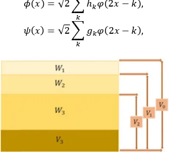
Figure 1. A together wit the whole sp
Adop
∑⊕
∈ℤ ≜ ⋯
y function (
on
= ⋯ + ( ) ∈ , ∀ ∈ ℤ
wavelet, then t orthogonal,
not necessar ace ⊆ (ℝ
… ⊕ ⊕
= ⊕ … ⊕
have the follo 1.… ⊆ ⊆
2. ⋃∈ℤ
3.⋂∈ℤ = {0
4. = +
5. ( ) ∈ ⟺
ence of subsp
∈ (ℝ) can the image bspace is
∈ (ℝ), then ed by the sam aces are ge ultiresolution paces encod
, whereas the ” features (det llows that eve in terms of th approximatin detailed funct e orthogonalit
s.
( ) = √2
( ) = √2
A sequence of m th their orthogo pace with the fin
pting the Multi
⊕ ⊕
) ∈ (ℝ) w
) + ( ) + ℤ . If is the subspaces
,
ily orthogona
ℝ)
… ⊕
⊕ ⊕
owing propert
⊆ ⊆ ⋯ ℤ = (ℝ) 0},
, ∈ ℤ, ⟺ (2 ) ∈
paces is ne n be approxi of the projec generated by n all of the s me function ,
enerated by th analysis at a de the “large s e subspaces
tails). ery function he approximat ng wavelet f tion can be b ty and the nest
(2 −
(2 −
multiresolution onal compleme nest data resolu
iresolution Wa
⊕ ... will have a uni
( ) + ⋯,
regarded as
∈ (ℝ)
. For ev al) we can
⊕ ,
. T ties:
⋯, ),
, ∈ ℤ.
ested. (see Fig imated with ction on . If
a single scal subspaces
in the same w he wavelet .
given scale (
scale” features represents
can uniquely ting and detai function and oth defined w ting propertie
),
),
nested subspac ent can constru ution avelet Analysis ique an are very the The g.1) any f the ling are way ( + s of the y be iled its with s of a pro as sub cou ano rep bas and by Fin the and the o for ∈ of ver ext com abi the we equ bas for equ wr ces uct
s in Radial Ba
for
(
and similar fo two-scale d operties
representing high pass an bspaces are c uld be transfo other. Under present any g ses of the emb
( ) = (
where,
( ) = ∑ ( ) = ∑ ∑
in which, the d . = .
. = ∑
Any refinable a series of nally, for any ere is a thresh d guarantees
( )‖ ≪ . eorem that sta on , denote
⟶ 0 in (ℝ
r all ∈ (ℝ) ∈ (ℝ), conv
In this section non-linear an ry successful tensively used mmon featur ility to keep th e speed and in e opt for the uation which i sed works of t Having been rm of the h uation shared ritten as follow
asis Functions
) = 2 (
ormula for ifference fun
( ) = 1 a
| ( )|
a band signal nd low pass f compactly sup ormed from o
the above given optional
bedded subspa
) + ( ),
. . +
∑ . . ,
refinement co
. can be c . .
e function c refinement y smooth func hold which
s its conver Note that c ates for all ∈
ed by , co
ℝ) [16]. It is a , the conver vergence is lo
Materials an
n, we confine isotropic PDE l in image d in image den
e of these e he essential ed ntensity of diff e non-linear is regarded as the field.
adopted as heat-diffusion d the similar ws.
to …
( ) (2 − )
. The scaling nction and and
∞,
l, that and filters, respec pported and t one level of conditions, w l function in aces as follow ∑ ∑ ≔ , . oefficients computed as . = ∑
can uniquely b coefficients, ction we w h puts a bound rgence, that convergence
∈ (ℝ), the onverges to
also worth me rgence is unif ocal and pointw
nd Methods
e our attention Es which have processing a noising and de equations is dges and take ffusion. Of the
version of s one of the m
an extended n equation,
r formalism
),
function is satisfies the
can serve ctively. These therefore data resolution to we can now terms of the ws. . . , ∞, . = . . . . be constructed called mask. will show that d on the error is, ‖ ( ) −
is derived a projection of , i.e., −
entioning that form whereas wise.
s
n over a group e proven to be and are thus eblurring. The their striking the control of ese equations, Perona-Malik ost cited PDE
Vol. 29 No.
where
= 0 is solutions bas difference o suggested. H compare the other method
First and form of the system. The on one hand vary across t that contain accuracy of form of RBF locally eval compartment are assessed removed. T privileges ov considerable makes the a incorporate a obtain an in first and then to compute levels of reso level. In this refinement an
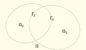
Given the initial cond implementati temporal dis grid which resolution. W method to fin Spatial discre domain Ω in boundary con (see Fig. 2) points are giv
4 Autumn 20
− ∇. ( (‖∇ ( . 0) = ( ) is the init
the Neuman sed on differe or finite ele Here, we will p output of to ds.
foremost, it i equation via aim is to spec d mediated by
the grid. So, ns the center our results, w F called adapt luated in ter t they represe d useful and This version
ver the class decreasing algorithm fas
adaptive RBF nitial mesh-fre n distribute it o the values of olution from t s case, we fol nd begin with nonlinear PD ditions, it is
ion of the pr scretization of is associated We thus set o nd the values etization is pe nto three par ndition and N
, namely, Ω
ven by
Figure 2. Dom 018
∇ ‖ )∇ ) = ( ), =
tial condition condition. Se ent methods (s ement metho propose a diffe o existing resu
s necessary to a replacing th
cify the coeffi y MRA and o
we begin wit rs. In order
we incorporat tive RBF in w rms of the ent. Centers o d kept and t
of RBF ha ic form, mos of computatio ster and more F to our meth ee solution u over the neste f the coeffici the coarsest l llow a recurs h the corset lev DE as well as
s conceivabl roposed meth f the solution d with the c out to employ
of the derivat erformed by d rts, which ar Neuman condit
Ω = Ω + Ω
main decomposi
A. Kh
0, = 0,
at time t=0 everal numer such as the fin ods) have b
erent method ults provided
o offer a discr hat into the R ficients which n the other h h creating a g
to increase te a more rec which centers gradient of of high gradie
he rest will as some cert st importantly ons that in t e optimized. hod, we need upon a base g ed spaces in or
ients at differ evel to the fin ive procedure vel.
its boundary e to start hod with spa n upon the ba coarsest level y the collocat tives on N nod
ividing the en re the bounda tion, successiv
where the g
ition hatoon Abadi, and rical nite been and d by
reet RBF are hand grid the cent are the ents be tain y, a turn To d to grid rder rent nest e of
and the atio-ased l of tion des. ntire ary, vely grid equ equ sys app tim res by on res res wil 2 2 der et al. Applying uations that ar
−
where = Δ
uation can als
which leads t
= − ( ( + 2 (
The system c stems assoc proximation o me step k afte
striction to the
. . Simi
Ω at the t striction to Γ
spectively. As ll be solved th
. = .
∇ . .
= 0, on
and,
. = .
∇ . .
= 0, on
For each no rivatives at ea
For the N +
= , = = , =
-scheme wi re discretized
= ∇. ( Δ . The right
o be expanded
∇. ( (‖∇ = (‖∇ ‖ + 2 (‖∇
o the followin
‖∇ ‖ )∇ ‖∇ ‖ )
= 0,
could now be iated with of the solution er n iteration
e artificial sub ilarly, the app time step k
Γ are denote s a result, our hrough two int
− ∇
. ∇ .
n Ω Γ⁄ , . = .
− ∇
. ∇ .
n Ω Γ⁄ , . = .
dal point, the ach node i and
( ) =
( ) =
L moving lea
J.
= 0. 1. … . , = 0. 1. … . .
ill yield th in terms of tim
(‖∇ ‖ )∇
t hand side o d and recappe
‖ )∇ ) ‖ )∇ ‖ ) ∇ ng system ∇ . ∇ ), on Ω.
e reduced to t the subdo n on subdom is denoted by bdomain Γ is proximation o after n itera ed by .
r boundary v nter-related sub
∇ . ∇
. ∇ . , in
, ,
∇ . ∇
. ∇ . , in
, on .
e first and s d point x are ob
( ) ,
( ) ,
ast squares no
Sci. I. R. Iran
he following me.
).
of the above ed as
. ∇ ,
in Ω,
two main sub omains. The main Ω at the y . whose s also denoted f the solution tions and its and .
value problem b problems.
. +
Ω ,
. +
Ω ,
econd partial btained as
odal points as
Adopting the Multiresolution Wavelet Analysis in Radial Basis Functions to …
well as the approximated values of the derivatives, we apply collocation method for all nodal points to gain the following equations.
= − ∇ ∇ +
2 ∇ ∇ . ∇ , where
( ) = ,
= ∑ ( + + +
+ ),
∇ = ∑ ( + ) , satisfying the Neumann condition for the boundary
nodes , j=N+1, . . ., N+L, for each subdomain, that is,
∑ = 0. To take the whole system forward, we run it
recursively with k=0, that is associated with our initial condition, = ( ). Hence, the problem is to solve an algebraic equation system ( ) ( )= ( ).
= − ∇ ∑ ( ) +
( ) + 2 ∇ ∑ +
+ + +
∑ ( ) + ( ) ,
( )= ,
We shall reiterate the above procedure until we nail an advisable time step. Then the solution ( , ) at each point of the domain ∈ Ω could be expressed as
( . ) ≈ ∑ ( ) ( ), ∈ Ω. Taking an initial solution at the coarsest level, we are going to apply the MRA by distributing it over the nested subspaces. The total account of the proposed
method is that both the smooth features of the picture are attributed to the wavelet coefficients at low levels whereas the highly-localized features are attributed to the wavelet coefficients at higher levels. Any irregularity or variation between the current level and the next coarse level can be depicted by the high values of the wavelet coefficients. It also allows us to make a decision over whether keeping or eliminating any wavelet coefficient that corresponds to some certain node of the domain. Using this adaptation scheme will result in keeping the essential nodes which collectively make a more optimal node distribution.
Results
To provide numerical example, we need to initialize the parameters and opt for a suitable numerical setting of RBF, that is, the type of radial functions we are going to use as well as an optimal node distribution method. To do so, we take into account a case where the system is fed up with the following parameters. We set up N=698 (the initial number of collocation nodes),
= 0.1 (shape parameter of radial basis functions) and
= 0.001 (the coarsest level of resolution).
Also, we will separately try both of MQRBF and Wendland polynomial all along our computations and the relevant comparison will be made at the final step. In order to compare the computational, error the and norms must be calculated are given as below. is a point wise norm taken over the domain while the Root Mean Square (in short RMS) is mean of the squares of the values, usually known for its
stability. We must show that the obtained solution approximates the exact solution of the operator equation (20). In sum, the algorithm that puts the whole system into practice could be elaborated as follows. The numerical results of the adaptive multiresolution wavelet scheme are given in Tables 1 and 2.
The errors are defined by,
= ess sup| ( ) − ( )|,
Table 1. Iterative progress of the adaptive multiresolution wavelet scheme (multiquadric function) from level 1 to 4.
N ( )
320 2.6831e+06 2.27E-02 4.18E-03
732 6.6004e+04 1.53E-01 2.79E-03
756 2.6018e+06 3.14E-02 1.43E-03
764 7.4874e+06 3.23E-03 1.62E-03
Table 2. Iterative progress of the adaptive multiresolution wavelet scheme (Wendland polynomial) from level to 4.
N ( )
320 7.4352e+04 1.41E+01 1.52E+01
764 2.1255e+06 7.03E-02 7.26E-03
980 6.51E+20 5.24E-01 2.79E-01
Vol. 29 No.
where approximated define the in
( )|.
More deta of the area is MQRBF and In additio
=
( , ) = ( , )
= Algorithm Select S, ∈
Put Ω = [ Set the grid Apply the ad
for j=
foreach cen Compute: th At finer leve Define and If , , t If , , t Solve the sy
( ) ( )=
Construct:
Set = Solve Use forward Find in [ Use forward End End
Algorithm
( ) ( )=
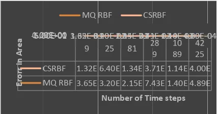
Figure 3. C different poi
C M -5.00.01.05.0
Erorr in
Are
a
4 Autumn 20
= 1 |
and d solutions re nfinity norm
ails can be fou s calculated as d CSRBF. on to the erro
= 0, , ∈
= 0, , ∈ [ , ∈ ℤ
, ] × [( − 1) [ , ] × [0, ] daptive MRA
: (j’s are all nter of the grid a he correspondin el + 1, , d apply the adap then remove , the keep , in ystem = ( )
, = an =
d -backward sub , ] × [( − 1) d -backward sub
1. Algorith = ( ).
Comparison be ints over time.
9
CSRBF 1.32E MQ RBF 3.65E 3.65E-03 1.32E-06 00E-01 00E+0000E-01 00E+00 MQ 018 ( ) −
are the espectively. O as = ess s
und in Fig. 3 in s a function of
or norms, the
∈ [ , ] × [0,
, ] × {0} , ] , = 1
l levels of resol at the j level, ng wavelet coef
ptive criteria from the grid the grid
nd P=permutati
bstitution to find , ] bstitution to find
hmic Solution
etween errors
25 81 2
6.40E 1.34E 3.7 3.20E 2.15E 7.4 01.20E-012.15E-017.43 01.40E-021.34E-023.71
Number of Tim
RBF CS
A. Kh
( )| ,
exact and Of course, we
sup| (
n which the er f time for both
accuracy of
] ,2, … ,
lution) , ∈ ℤ fficient ,
d
on matrix
d
d
of the syste
of two RBFs 28 9 10 89 42 25 71E 1.14E 4.00E 43E 1.40E 4.89E 3E-021.40E-024.89E-0 1E-031.14E-034.00E-0
me steps RBF hatoon Abadi, the can ) − rror h of the me ord b res us spa def sat ana app sat
if 0
spa seq ∈ ope poi sat app tha by our em at E E 04 04 et al.
ethod can als der of approxi belongs to th sults in Sobol cast a quick ace.
Definition 1
fined by the tisfying
‖ ‖ ≡
The followin alysis (see, [1
Theorem 1.
proximation s tisfies
∃ 0, | ( ( )
and also,
∃ 0,
Put =
0 we
( ) ∈ ⇔
Consider a B ace G, and a quence has or
∈ , ‖( −
erator norm, w
for some a
Definition 2. intwise order
if for any tisfies
‖ ‖ ≡ ‖
as tends t proximation s at this relation
Now, by the the functions
∈
Also, for a s r method, the
o be easily e imation [17].
e Sobolov sp ov spaces. Be
glance at the
. The Sobole set of those
( ) (1
ng results cou 8], for proofs
Suppose (
such that the
) | (1 + | = 0, for 1
( )
(1 − ( ) . T have
⇔ ∑ 2
Banach space sequence of rder of approx
) ‖ (
we have
‖( − )‖ and each .
MRA { } o of approxima
∈ , the n-th
( − ) ‖
to infinity. It s in if s i n holds, for all
above results of our proble
∈ ⇔
et of refinabl e order of app
J.
evaluated in Since the defi pace, we need efore alluding e definition of
ev Space e functions
1 + | | )
uld be used and more det
)∈ℤ be a m
associated fu
| |) ,
+ 1,
+ | |) ,
Then for all (
+∞.
e K and a n f operators
ximation ( ( ) if and on
( ),
or wavelet fam ation (or conv
h order appro
= (2 ), t yields the b is the largest l ∈ .
whose constr em we get,
2 +∞
le answers ’s proximation i
Sci. I. R. Iran
terms of the finable answer d to use some g to those, let f the Sobolov
of order is
( ) ∈ ( )
∞
for the error tails).
multiresolution function ( )
.
( ) ∈ (ℝ) ,
normed linear
: → , the
), i.e., for all nly if for the
mily yields vergence) s in oximation
best order of number such
raints are met
∞.
s, attained by s (2 ). To
elaborate m projected ov since the req the existence error estimat
‖ ‖ =
where (
( , ). On approximatio norm that de
− ( )
the function theory is to e a priori kno conversely, d convergence
It must be set of RBF c of a dense m coarse mesh conditioned mesh near t allows the re specified val illustration algorithm, se the results o same problem order of our RBF and w surpasses tha stated in [20] It implies sheer RBF. B Volume Met as ( ) [21] meshless me Method to s eliminating t order of app slower than o method conv level set me Malik Equat order of app Indeed, our m method amo therefore req reach the solu
Adop
more, given a ver the refinab quired conditio e of a constan tion for approx
‖ ‖
= (2 ), (a shape param ne must keep on lies at the emonstrates th
, where . A classic estimate the co owledge on
derive the sm rate of . e noted that s centers our app mesh near the
h is maintain system will the boundarie esulted conditi lue that guara
of nodal di ee Figs. 4 and of similar mes m, it could be method, that wavelet basi at of the stand
].
that our mo Besides, the m thod which co ]. Also, Mei a ethod, called solve the Pe the boundary proximation is ours as it grow verges expone ethod has also tion [23] and proximation u method with t ong the meth
quires the le ution.
pting the Multi
a smooth fu ble spaces, i.e ons stated in [ nt is guaran
ximation of
2 ‖ ‖
meter) depend p in mind th e heart of a s he degree of pr
( ) is an ap cal problem i
onvergence ra the smoothne moothness of
tarting from f proach leads
boundaries, w ned elsewher
be assigned es. Furthermo ion number to antees a stable istribution in d 5). Finally, i sh free metho shown that th stems from th is equals to dard RBF that
odel is more e method is also
onverges to th and Zhu [22] the Homoto rona-Malik e y effect and s (4 ), wh
ws polynomia entially. The o been used t d the authors using this m the order (2
hods introdu ast number o
iresolution Wa
nction ∈
e. = +
[19] are satisf
nteed so that are as follow
,
ds on the funct hat the order simple differe recision, nam pproximation n approximat ate of based ess of ( ),
( ) out of
finely distribu to the generat while a relativ re. A highly to the very f ore, the meth o be lower tha e solution (for n the propo in comparison od applied to
he approximat he assimilation o (2 ), wh t is ( log )
efficient that faster than Fin e solution as , applied anot opy Perturbat equation throu
showed that hich is obviou
ally, whereas fast progress to solve Pero proved that method is (
2 ) is the fas uced so far
of operations
avelet Analysis , fied, the ws: tion r of ence mely, for tion d on
, or the
uted tion vely y ill fine hod an a r an osed n to the tion n of hich
) as
the nite fast ther tion ugh the usly our sing ona-the ). stest and s to
the con ord sch RB it m cas itse pro dif res of usu adv
s in Radial Ba
We proposed e nonlinear Pe nverges to th der compared heme was mai BF grid by the must be noted se when the c elf by Catte-ovided here fferent layers solution, and t
the spectrum ual RBF meth vantage could
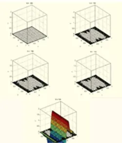
Figure 4. (l distribution technique as proposed algo
Figure 5. (r distribution technique as proposed al function.
asis Functions
Discu
d an adaptive erona- Malik e e solution wi d to the exist
inly relied on virtue of the d that the met convolution a -Lion equatio is akin to a , each repres thus the soluti m to the other hod, no mesh h d supposedly
left) A schem produced by well as the ch orithm using mu
ight) A schem produced by well as the ch lgorithm using
to …
ussion
e wavelet met equation and s ith a higher a sting methods creating and p wavelet basis thod must be appears inside on [24]. The a spectrum senting certa tion can shift r. Furthermor has been gene be applied in
matic illustratio y the wavele hosen RBF cen multiquadratic fu
matic illustratio y the wavele hosen RBF cen ng Wedland
thod to solve showed that it approximation s. The whole pertaining the s. Nonetheless tested for the e the gradient solution we that contains ain degree of from one end re, as for any erated and this n 3D cases as
n of nodal et adaptive nters by the unction.
Vol. 29 No. 4 Autumn 2018 A. Khatoon Abadi, et al. J. Sci. I. R. Iran
well as the problems that demand re-meshing of the space all along the computations. It should be noted that the larger the time intervals, the more instability the system will experience, but as the comparative computations suggest, instability would be less pronounced if the adaptive wavelet CSRBF method is used.
Conclusion
Finally, our method is fairly optimized and easy to implement. Besides, the wavelet transformations can be engaged more directly in the course of the computation via building a sequence of bounded wavelets to approximate the solution, albeit the ultimate shape of the exact solution is not quite regular and therefore easily prone to fit in.
Acknowledgement
This work was part of the PhD thesis of the first author supported by Tarbiat Modares University.
References
1. Moody J. and Darken C. Fast learning in networks of locally-tuned processing units. Neural Computation1 :281-294 (1989).
2. Yee P. and Haykin S. A Dynamic regularized Gaussian radial basis function network for nonlinear nonstationary time series prediction. IEEE Signal Processing Society 47(9): 2503-2521 (1999).
3. Buhmann M. D. Radial basis functions. Cambridge University Press, Cambridge (2003).
4. Uhlir K. and Skala V. Radial basis function use for the restoration of damaged images. Computer Vision and Graphics. In: Computational Imaging and Vision book series (CIVI, volume 32)pp.839-844 (2006).
5. Amattouch M.R. Belhadj and H. Nabila, A modified fixed point method for the Perona-Malik equation, Journal of Mathematics and System Science7: 175-185 (2017). 6. Guidotti P. Kim Y. and Lambers J. Image restoration with
a new class of forward-backward-forward diffusion equations of Perona–Malik type with applications to satellite image enhancement, SIAM J. Imaging Sci. 6: 1416–1444 (2013).
7. Guo Z. Sun J. Zhang D. and Wu B. Adaptive Perona– Malik model based on the variable exponent for image denoising, IEEE Trans. Image Process 21: 958–967 (2012),
8. Mescheder L.M. and Lorenz D.A. An extended Perona– Malik model based on probabilistic models, J Math Imaging and Vsiion60: 128–144 (2018).
9. Maiseli B. Msuya H. Kessy S. and Kisangiri M. Perona– Malik model with self-adjusting shape-defining constant, Information Processing Letters 137:26-32 (2018). 10.Vrankar L. Ali Libre N. Ling L. Turk G. and Runovc. F.
Solving moving-boundary problems with the wavelet adaptive radial basis functions method. Computers & Fluids 86: 37-44 (2013).
11.Blu T. and Unser M. Wavelets, fractals, and radial basis functions. IEEE Transactions on Signal Processing 50: 543-553 (2002).
12.Rannacher R. and Wendland W.L. On the order of pointwise convergence of some boundary element methods. Part II: Operators of positive order. Math. Modeling Numer. Anal.22:343-362 (1988).
13.Larsson E. and Fornberg B. A numerical study of some radial basis function based solution methods for elliptic PDEs. Computers Math. Appl.46: 891-902 (2003). 14.Meyer Y. Wavelets and operators. Cambridge Univ. Press,
Cambridge (1992).
15.Mallat S. A wavelet tour of signal processing. Academic Press, New York (1999).
16.Unser M. A. and Blu T. A. Comparison of wavelets from the point of view of their approximation error. Proc. SPIE 3458. In: Wavelet Applications in Signal and Image Processing VI, ed. A F Laine, M A Unser, A Aldroubi (1998).
17.Debnath L. Wavelet transforms and time-frequency signal analysis. Birkhäuser, Boston (2001).
18.Kelly S.E. Kon M.A. and Raphael L.A. Local convergence for wavelet expansion. J. Func. Anal.126: 102-138 (1994). 19.Zhongying C. Micchelli C.A. and Yuesheng X. A multilevel method for solving operator equations. Journal of Mathematical Analysis and Applications262: 688–699 (2001).
20.Kamranian M. Dehghan M. and Tatari. M. An image denoising approach based on a meshfree method and the domain decomposition technique. Engineering Analysis with Boundary Elements39: 101-110 (2014).
21.Handlovtčová A. and Krivá Z. Error estimates for finite volume scheme for Perona-Malik equation. Acta Math. Univ. Comenianae LXXIV: 79-94 (2005).
22.Mei S.L. and Zhu. D.H. HPM-based dynamic sparse grid approach for Perona-Malik equation. Scientific World Journal, 417486 (2014).
23.Rumpf M. and Preusser T. A level set method for anisotropic geometric diffusion in 3D image processing. SIAM J. Appl. Math.62(5): 1772-1793(2006).