Optimal Control of the Vehicle Path Following by Using Image Processing Approach

Please cite this article as: Y. Pourasad, Optimal Control of the Vehicle Path Following by Using Image Processing Approach, International Journal of Engineering (IJE), IJE TRANSACTIONS C: Aspects Vol. 31, No. 9, (September 2018) 1559-1567

International Journal of Engineering

Optimal Control of the Vehicle Path Following by Using Image Processing Approach

Y. Pourasad*

Faculty of Electrical Engineering, Urmia university of Technology, Urmia, Iran

P A P E R I N F O

Paper history:

Received 11 November 2017

Received in revised form 13 December 2017 Accepted 17 Januray 2018

Keywords: Trailer Image Processing Path Following Steerability Optimal Control

A B S T R A C T

Nowadays, the importance of the vehicles and its dramatic effects on transportation system is obvious. The use of trailers with multiple axels for transporting bulky and heavy equipment is essential. Stability and steerability of trailers with multiple axels and wheels is one of the main concerns in the transportation system. Therefore, in this paper dynamic modeling and control of a 5 axial trailer was studied. As well as to increase maneuverability and speed up, 3 axles was considered to be steered. Also, by using image processing trailer path following in desired path with the highest accuracy was achieved. In this study, first a 14 DoF model for a 5 axial trailer with 3 steering axles was considered and its dynamic was formulated. For this purpose, dynamic equations including kinematic and kinetic of trailer was obtained. Then, with evaluating trailers response, a linear quadratic optimal control algorithm was designed. In order to evaluate the performance of the control algorithm, control problem simulation for single lane change and overtaking was done. The results confirmed the performance of designed control algorithm and image processing accuracy in trailer path following.

doi: 10.5829/ije.2018.31.09c.12

1. INTRODUCTION1

In the last two decades, the use of articulated tracked vehicles has increased dramatically. The reason for this is the restrictions on driving single tracked vehicles. Today, articulated tracked vehicles are widely used in industries. Articulated tracked vehicles can be used as transporter, heavy equipment [1] or in agriculture field [2]. They can be used as desert transporters or carriers of passengers on the snow or sand terrains. They can also be used as forest fire tracked vehicles [3]. In addition to the reasons and as the most important reason, they can be used invaluable in the field of military vehicles for pulling tracked trailers and towing knocked out tanks from the battlefield [4]. Maneuverability articulated tracked vehicles can be excellent, because it usually needs less power to bypass than single tracked vehicles. Improving obstacle crossing and uniform ground pressure are the benefits of articulation to towing vehicles [5, 6]. A lot of ease is created by articulation, because it allows the path to match the ground, resulting in more integrated pressure. Slender vehicles are less likely to be at the same level of contact with obstacles and less

*Corresponding Author Email: [email protected] (Y. Pourasad)

resistance to short and wider vehicles. Although there is a straightening up problem when steering a car. This problem occurs in the wagon type of articulated tracked vehicles [7]. Alhimdani and his colleagues [8] try to solve this problem in theory the use of a hydraulic piston. Although it was found that this method is not practical and practical, the problem has not been completely solved yet. A new idea for the steering problem was suggested during the right maneuvering of a towed vehicle, and it was the use of high tension ropes (high strength) to tow a trailer chasing trailer by a towing vehicle [9]. Two loose ropes were used when they were bypassed, when straightening up one of the ropes was pulled. Luijten [10] in addition to the conventional combinations of tractor-semi-trailer, truck - central axle trailer, truck-full trailer, ecomobies; taller and heavier truck combinations; as a test and experience in the Netherlands. Safety is a common concern among all road users, challenged by the volume of traffic that has actually grown in recent years and is projected to rise further in the future.

2. RESEARCH METHOD

Modeling in fact means extracting mathematical equations of the behavior of a system and approximating the system's behavior by those equations. For example, different vehicle behaviors such as side and side behavior, longitudinal function, travel comfort, etc. can be approximated using a number of state-space equations, whose state variables are the same degrees of system freedom or derivatives. Modeling of automobile dynamic equations can be divided into two general categories: a) simple linear modeling and b) complex nonlinear modeling. Usually, a simple linear model for designing a system for maintaining the rotational stability of a vehicle using a steering input is used first, so that the design and implementation of the control system can be done at a lower cost. Then, considering that the behavior of the vehicle is highly nonlinear and cannot be used, a simple linear model to achieve the behavior of the vehicle in all its operating conditions, is used in a more complex model with more degrees of freedom to simulate vehicle behavior.

2. 1. Trailer Kinematics In this section, the velocity

and velocity are calculated according to the defined coordinate devices. Using the kinematics of the system, in other words, the system's transition and rotational velocities, kinetic energy, acceleration, kinetics and equations of motion of the system will be computable.

The objective in modeling is to evaluate the axial motion of the 5-axis trailer movement, which is visible in Figure 1 in its lateral view, and the upper. As shown in Figure 2, axes 1, 4, and 5 have the ability to steer. According to Figure 1 and coordinate devices, we will have:

(1(

[i_jn

n] = [

cos θ2 − sin θ2

sin θ2 cos θ2] [

iu

ju]

)2(

[

iu

ju

ku

] = [

1 0 0

0 1 −φ

0 φ 1

] [

is2

js2

ks2

]

)3(

𝐕𝐂𝐆𝟐= ẋn𝐢𝐧+ ẏn𝐣𝐧

)4(

𝐕𝐂𝐆𝟐= 𝐱̇𝐮𝐢𝐮+ 𝐲̇𝐮𝐣𝐮

)5)

ẋn= ẋucos θ2− ẏusin θ2

)6(

ẏn= ẋusin θ2+ ẏucos θ2

as semi-trailer as the basis for their studies. For this purpose, they have developed two dynamic models in the lateral control of a trailer - semi-trailer; a complex simulation model and two simplified control models. In their report, a complex nonlinear model has been developed to simulate the dynamic responses of tractor-to-trailer vehicles, which has been used to evaluate the efficiency of the lateral control algorithm. The articulated vehicle is most commonly composed of two main parts of the tractor unit and trailer unit. Due to the more complex dynamical structure and the height of the center of gravity, they have a more detailed car than a riding vehicle have less motor stability [12, 13]. Schmid [14] studied the dynamical stability of a tractor-trailer by analyzing linear equations. He has used the Routh Hurwitz Criteria to detect and instability. An analysis by Fakoor et al. [15] has shown that the nominal position of the center of gravity in path following is one of the most important parameters in the stability. In existing research, the stability analysis of heavy vehicles is usually carried out using the two main methods of Routh Hurwitz and the solution of the specific value of the characteristic equation. Fakoor et al. [16] have examined the stability profile of the robot using special values analysis. They have developed a set of algebraic equations for determining the stability ranges of a trailer-mounted system. In his research, the general rule governing both oscillatory and non-volatile stability is derived using the Routh Hurwitz benchmark. The graphical expression of this analysis is presented as a stable region bounded by stable oscillatory boundaries and non-oscillatory stability. But it should be noted that increasing the number of axles and, in the long run, the trailer wheels will consider certain considerations for increasing the speed of transport, increased maneuverability, increased safety and better control, which will reduce the high cost of the SUV tires. Therefore, dynamic modeling and control of a 5-axle trailer have been investigated. Also, to increase maneuverability and increase the speed and speed of the vehicle's route, the 3-axis steering of the trailer (axis 1, 4 and 5) was considered. In this paper, we first consider a 14-degree freedom model for a 5-axle trailer with 3 steering axles, and its characteristics are described. Then, the trajectory dynamics equations are extracted from the kinematic and kinetic equations. In this paper, an optimal linear square optimization algorithm is designed to examine the type of trailer behavior. Eventually, using the image processing algorithm, the path of the vehicle is identified along the road and is designed using the controller and the input of the road route from the algorithm of image processing, routing, and trailer movement. To test the performance of the control algorithm, the control problem is simulated for three single line switching maneuvers, dual line switching, and overtaking. The results confirm the validity of the control algorithm.

The trailer speed in each of the reference and unscreened coordinate systems will be in accordance with Equations (3) and (4), which is obtained by Equations (1) in (5) and (6).

Figure 1. Trailer Planar movement

Figure 2. Trailer side schematic

)7)

𝐚𝐂𝐆𝟐= ẍn𝐢𝐧+ ÿn𝐣𝐧

)8(

𝐚𝐂𝐆𝟐= (ẍu− ẏuθ̇2)𝐢𝐮+ (ÿu+ ẋuθ̇2)𝐣𝐮

)9(

ẍn= (ẍu− ẏuθ̇2) cos θ2− (ÿu+ ẋuθ̇2) sin θ2

)10(

ÿn= (ẍu− ẏuθ̇2) sin θ2+ (ÿu+ ẋuθ̇2) cos θ2

The angular velocity of the mass coordinate system with the ratio of the spring to the reference device is calculated according to Equation (11).

)11(

𝛚𝐬𝟐⁄𝐧= φ̇𝐢𝐬𝟐+ φθ̇2𝐣𝐬𝟐+ θ̇2𝐤𝐬𝟐

By deriving from each vector the coordinates of the system are:

)12(

d

dt𝐢𝐬𝟐= 𝛚𝐬𝟐⁄𝐧× 𝐢𝐬𝟐= (φ̇𝐢𝐬𝟐+ φθ̇2𝐣𝐬𝟐+ θ̇2𝐤𝐬𝟐) ×

𝐢𝐬𝟐= θ̇2𝐣𝐬𝟐− φθ̇2𝐤𝐬𝟐

)13(

d

dt𝐣𝐬𝟐= 𝛚𝐬𝟐⁄𝐧× 𝐣𝐬𝟐= (φ̇𝐢𝐬𝟐+ φθ̇2𝐣𝐬𝟐+ θ̇2𝐤𝐬𝟐) ×

𝐣𝐬𝟐= −θ̇2𝐢𝐬𝟐+ φ̇𝐤𝐬𝟐

)14)

d

dt𝐤𝐬𝟐= 𝛚𝐬𝟐⁄𝐧× 𝐤𝐬𝟐= (φ̇𝐢𝐬𝟐+ φθ̇2𝐣𝐬𝟐+

θ̇2𝐤𝐬𝟐) × 𝐤𝐬𝟐= φθ̇2𝐢𝐬𝟐− φ̇𝐣𝐬𝟐

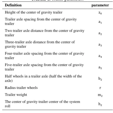
The trailer parameters shown in Figure 2 are presented in Table 1.

Now, according to the calculations done and the relationship between the coordinate devices, the overall speed of the trailer is calculated as follows.

)15(

𝐯𝐂𝐆𝟐⁄𝐧= ẋn𝐢𝐧+ ẏn𝐣𝐧+ h2φθ̇2𝐢𝐬𝟐− h2φ̇𝐣𝐬𝟐

TABLE 1. Trailer parameters

parameter Definition

z0

Height of the center of gravity trailer

a1

Trailer axle spacing from the center of gravity trailer

a2

Two trailer axle distance from the center of gravity trailer

a3

Three-trailer axle distance from the center of gravity trailer

a4

Four-trailer axle spacing from the center of gravity trailer

a5

Five-trailer axle spacing from the center of gravity trailer

b2

Half wheels in a trailer axle (half the width of the axle)

r Radius trailer wheels

m2

Trailer weight

h2

The center of gravity trailer center of the system roll

)16(

𝐯𝐂𝐆𝟐⁄𝐧= (ẋncos θ2+ ẏnsin θ2+ h2φθ̇2)𝐢𝐬𝟐+

(−ẋ_nsin θ2+ ẏncos θ2− h2φ̇)𝐣𝐬𝟐+

φ(ẋnsin θ2− ẏncos θ2)𝐤𝐬𝟐

2. 2. Trailer Kinetics As shown in Figure 6, the model

for a trailer is a 14 degree freedom model. Generalized system coordinates 10 axis of the wheel corresponding to 10 wheels, xn the position of the center of gravity of the

trailer in the direction of the axis xn, yn the position of

the center of gravity of the trailer in the direction of the yn axis, the tractor roller angle φ and Yaw trailer angle

θ2. The generalized coordinates that can be analyzed with

the behavior of the system are as follows.

)17(

q = [xn yn φ θ2]T

)18(

d dt(

∂ℒ

∂q̇k) − (

∂ℒ ∂qk) +

∂F ∂q̇k= fk

Where qk is the generalized k-th and Lagrange ℒ

coordinate difference between the kinetic energy T and the potential fk is the generalized k-th force.

)19(

ℒ(q, q̇) = T(q, q̇) − U(q) =1

2q̇

T_{B(q)q̇ − U(q)}

B (q) is a positive mechanical inertia matrix of the mechanical system.

)20(

F =1

2∑ ∑ crsq̇rq̇s n

s=1 n

r=1

The kinetic energy of the system is equal to:

)21(

T =1

2m2vCG1⁄n. vCG2⁄n+

1

2ωs2⁄n. I2. ωs2⁄n

The potential energy of the system will be equal to:

)22(

U(q) =1

2kφφ 2_{− m}

2gh2(1 − cos φ)

And F is as follows:

)23(

F =1

2cφφ̇ 2

By calculating and simplifying, the equations of motion of the system in the system of low-intensity mass coordinates are calculated as follows:

)24)

m2(ẍu+ h2φθ̈2− ẏuθ̇2+ 2h2φ̇θ̇2) = Fxu

)25(

m2(ÿu− h2φ̈ + ẋuθ̇2+ h2φθ̇22) = Fyu

)27(

m2h2φẍu+ (Iz+ (Iy+ m2h22)φ2)θ̈2−

m2h2φẏuθ̇2+ 2(Iy+ m2h22)φφ̇θ̇2= Fθ2

So, with this in mind, we are going to retrieve the generalized forces in the system of bumpy mass coordinates. The generalized force for xu is as follows.

(28)

Fxu= fatcos(θ2− θ1) + fbtsin(θ2− θ1) +

(fa11+ fa12) cos δ1+ (fb11+ fb12) sin δ1+

(f_a21+ fa22) + (fa31+ fa32) + (fa41+

fa42) cos δ4+ (fb41+ fb42) sin δ4+ (fa51+

fa52) cos δ5+ (fb51+ fb52) sin δ5

The generalized force for 𝑦𝑢 is as follows.

)29(

𝐹𝑦𝑢= −𝑓𝑎𝑡𝑠𝑖𝑛(𝜃2− 𝜃1) + 𝑓𝑏𝑡𝑐𝑜𝑠(𝜃2− 𝜃1) +

(𝑓𝑎11+ 𝑓𝑎12) 𝑠𝑖𝑛 𝛿1+ (𝑓𝑏11+ 𝑓𝑏12) 𝑐𝑜𝑠 𝛿1+

(𝑓𝑏21+ 𝑓𝑏22) + (𝑓𝑏31+ 𝑓𝑏32) + (𝑓𝑎41+

𝑓𝑎42) 𝑠𝑖𝑛 𝛿4+ (𝑓𝑏41+ 𝑓𝑏42) 𝑐𝑜𝑠 𝛿4+ (𝑓𝑎51+

𝑓𝑎52) 𝑠𝑖𝑛 𝛿5+ (𝑓𝑏51+ 𝑓𝑏52) 𝑐𝑜𝑠 𝛿5

The generalized force for φ is as follows.

)30(

𝑓𝜑= (𝑓𝑏11(𝑧0𝑐𝑜𝑠 𝜑) + 𝑓𝑏12(𝑧0𝑐𝑜𝑠 𝜑)) +

(𝑓𝑏21(𝑧0𝑐𝑜𝑠 𝜑) + 𝑓𝑏22(𝑧0𝑐𝑜𝑠 𝜑)) +

(𝑓𝑏31(𝑧0𝑐𝑜𝑠 𝜑) + 𝑓𝑏32(𝑧0𝑐𝑜𝑠 𝜑)) +

(𝑓𝑏41(𝑧0𝑐𝑜𝑠 𝜑) + 𝑓𝑏42(𝑧0𝑐𝑜𝑠 𝜑)) +

(𝑓𝑏51(𝑧0𝑐𝑜𝑠 𝜑) + 𝑓𝑏52(𝑧0𝑐𝑜𝑠 𝜑))

The generalized force for 𝜃2 is as follows.

)31(

𝑓𝜃2 = (𝑓𝑏𝑡𝑐𝑜𝑠(𝜃2− 𝜃1) − 𝑓𝑎𝑡𝑠𝑖𝑛(𝜃2− 𝜃1))𝑙 +

(𝑓𝑏11+ 𝑓𝑏12)𝑎1+ (𝑓𝑏21+ 𝑓𝑏22)𝑎2+ (𝑓𝑏31+

𝑓𝑏32)𝑎3+ (𝑓𝑏41+ 𝑓𝑏42)𝑎4+ (𝑓𝑏51+ 𝑓𝑏52)𝑎5+

(𝑓𝑎12− 𝑓𝑎11)𝑏2+ (𝑓𝑎22− 𝑓𝑎21)𝑏2+ (𝑓𝑎32−

𝑓𝑎31)𝑏2+ (𝑓𝑎42− 𝑓𝑎41)𝑏2+ (𝑓𝑎52− 𝑓𝑎51)𝑏2

3. DESIGNING A CONTROL ALGORITHM

The main purpose of this section is to design a control algorithm for lateral control of the system. For this purpose, a linearized model of the trailer dynamics is firstly extracted. Then, based on this linear model, an optimal linear square control algorithm is designed.

3. 1. Trailer Dynamics and its Linearization To

extract the dynamic model, the trailer is operated as follows:

(32)

𝑚2(𝑦̈𝑢+ 𝑥̇𝑢𝜃̇2) = 𝐹𝑦𝑢

(33)

𝐼𝑧𝜃̈2= 𝐹𝜃2

Given 𝑥̇𝑢= 𝑢 , 𝑦̇𝑢= 𝑣 and 𝜃̇2= 𝑟 we will have:

(34)

𝑚2(𝑣̇ + 𝑢𝑟) = 𝐹𝑦𝑢

(35)

𝐼𝑧𝑟̇ = 𝐹𝜃2

To get the state of the system state, the system state variables are defined as follows.

(36)

{

𝑥1= 𝑦𝑢

𝑥2= 𝑦̇𝑢

𝑥3= 𝜃1

𝑥4= 𝜃̇1

→

{

𝑥̇1= 𝑥2

𝑥̇2= −𝑢𝑥4+

1 𝑚2𝐹𝑦𝑢

𝑥̇3= 𝑥3

𝑥̇4=_𝐼1

𝑧𝐹𝜃2

With linearization, simplification, and computing we will:

(37)

𝑥̇1= 𝑥2

(38)

𝑥̇2= −𝑢𝑥4+_𝑚1

2{−

2

𝑢(𝑐1+ 𝑐2+ 𝑐3+ 𝑐4+

𝑐5)𝑥2−

2

𝑢(𝑐1𝑎1+ 𝑐2𝑎2− 𝑐3𝑎3− 𝑐4𝑎4−

𝑐5𝑎5)𝑥4+ 2𝑐1𝛿1+ 2𝑐4𝛿4+ 2𝑐5𝛿5}

(39)

𝑥̇3= 𝑥4

(40)

𝑥̇4=

1 𝐼𝑧{−

2

𝑢(𝑐1𝑎1+ 𝑐2𝑎2− 𝑐3𝑎3− 𝑐4𝑎4−

𝑐5𝑎5)𝑥4+

2 𝑢(𝑐1𝑎1

2_{+ 𝑐}

2𝑎22− 𝑐3𝑎32− 𝑐4𝑎42−

𝑐5𝑎52)𝑥4+ 2𝑐1𝛿1− 2𝑐4𝛿4− 2𝑐5𝛿5}

Regarding the linearization, we will have in state matrix:

(41)

where in:

(42)

𝐴 = [

0 1 0 0

0 −1.0836 0 −15.5834

0 0 0 1

0 0.1507 0 −0.7534

]

(43)

B = [

0 0 0

3.6122 3.6122 3.6122

0 0 0

1.5069 −1.5069 −2.5115

]

(44)

C = [

1 0 0 0

0 1 0 0

0 0 1 0

0 0 0 1

], D=0

3. 2. Linear Quadratic Optimal Control Linear

square control optimal method is one of the most important optimal design methods in linear systems. The advantage of this method is the state vector feedback control method, which provides a systematic method for calculating the state vector feedback control matrix.

3. 2. 1. Linear Quadratic Regulator: Consider the

Linear Time Invariant (LTI) system ofẋ = Ax + Bu, the goal is to obtain the k-state vector feedback control u(t) = −kx, in such a way that the following performance index is minimized.

)45(

J = ∫ (x∞ T_{Qx + u}T_Ru)dt

0

By inserting u(t) = −kx we will have:

)46(

J = ∫ x∞ T_{(Q + k}T_Rk)xdt

0

For the above problem to be answered, the controller must first be stable. Therefore, at least unstable modes must be stable or, in a more comprehensive state of the system, must be controlled.

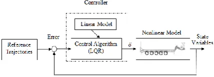
To better understand the control algorithm, the control diagram of Figure 4 can provide the correct image of the control system.

3. 3. Image Processing

3. 3. 1. Image Processing Consists Essentially of the Following Three Steps

 Capture images with optical scanners or with cameras and digital sensors

Figure 4. optimal control application

 Image analysis and manipulation, including: data compression, image restoration and extraction of specific information from the image by the image processing process

 The last step in which the output result can be an image or a report of the information that was obtained at the stage of the analysis of the image in the previous step.

The purpose of the image processing in this paper is to provide an independent input system for the vehicle's routing control system, which includes image intensification and recovery, image retrieval, pattern measurement, image recognition, and the transmission of roadway information to the controller input (Figure 5).

For vehicle routing, using sensors mounted on a vehicle, the road profile is marked on the road and obstacle lines on the specified route, and the vehicle can accurately navigate the vehicle's path by adjusting the steering wheel and torque. Two pieces of information are extracted from the image: offset the path from the center of the image and the path gradient. Figure 6 shows the extraction feature in more detail. The image processing system output is used as an input for the controller. The solution used here is to use a proper command control, which is guided by a combination of outputs of the image processing step. The only changes required when changing the chassis type to the engine control functions and mapping between the output of the image processing step and the vehicle commands. Obviously, if the vehicle is on the left side of the image, it should turn to the left, so if the vehicle is on the right, it should go back to the right, and also have to rotate the path in the image. Figure 7 shows the process of image processing of the road with lines on it.

4. RESULTS

4. 1. Uncontrolled system behavior In this

section, the behavior of the system is examined without controller, for this purpose the system response is calculated to the initial conditions without controller presence. The results are shown in Figures 8 to 10. What is clear from the results is that the response was unstable, indicating the need for a controller to be present.

Figure 6. Road image processing

4. 2. System Control Response to the Initial

Conditions The response to its initial conditions is

also presented in Figures 9 and 10. The results obtained in comparison with the results of the previous section indicate the optimal performance of the designed control algorithm.

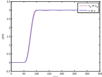
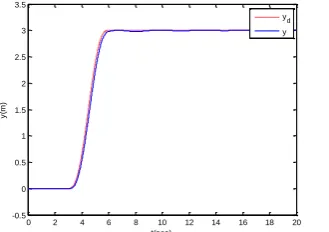
4. 3. Simulation for Standard Maneuvers

Considering the maneuver of replacing the single line for the trailer and performing the simulation of the results, the following is presented in Figures 11 to 20. What is clear from the results is the effectiveness of the control algorithm in controlling the trailer on this maneuver.

As shown in figure 16, the vehicle deviation from desired path remains below 0.1m over the lane change path while the heading error over the maneuver is less than 0.2 rad.

Figure 7. The variable y trailer position response in the vertical direction without a controller

Figure 8. The variable θ (yaw) response of the trailer in the vertical direction without the controller

Figure 9. Variable response y of the trailer position in the vertical direction relative to the initial condition

Figure 10. Variable response y ̇ ̇of the trailer on the horizons page relative to the initial conditions

It shows the accuracy of proposed controller and image processing system in trailer path following.

Figure 11. Single trailer line shift maneuver on Vehicle

0 1 2 3 4 5 6 7 8 9 10

0 0.05 0.1 0.15 0.2 0.25 0.3 0.35 0.4

t(sec)

y

(m

)

0 1 2 3 4 5 6 7 8 9 10

-0.01 0 0.01 0.02 0.03 0.04 0.05 0.06

t(sec)

d

(r

a

d

/s

)

0 50 100 150 200 250 300 350

-0.5 0 0.5 1 1.5 2 2.5 3 3.5

x(m)

y

(m

)

Figure 12. Fourth axis of the trailer command in the single line switching maneuver (control input)

Figure 13. Trailer side position diagram in time in the single line switching maneuver

Figure 14. Yaw Trailer Angle Scale Based on Time in the single line switching maneuver

Figure 15. Timing of the Yaw (angular velocity) of the trailer in time in the single line switching maneuver

Figure 16. Trailer roll rate graph in time in the single line switching maneuver

Figure 17. The slip angle of the first axle trailer in terms of time in the single line switching maneuver

Figure 18. The slip angle of the second axle trailer in terms of time in the single line switching maneuver

Figure 19. The slip angle of the third axle trailer in terms of time in the single line switching maneuver

0 2 4 6 8 10 12 14 16 18 20

-0.02 0 0.02 0.04 0.06 0.08 0.1 0.12 0.14 0.16

t(sec)

4

₄

0 2 4 6 8 10 12 14 16 18 20 -0.5

0 0.5 1 1.5 2 2.5 3 3.5

t(sec)

y

(m

)

yd y

0 2 4 6 8 10 12 14 16 18 20

-0.08 -0.07 -0.06 -0.05 -0.04 -0.03 -0.02 -0.01 0 0.01

t(sec)



(r

a

d

)



0 2 4 6 8 10 12 14 16 18 20

-0.08 -0.06 -0.04 -0.02 0 0.02 0.04 0.06 0.08

t(sec)

d

(r

a

d

/s

)

d

0 2 4 6 8 10 12 14 16 18 20

-0.4 -0.3 -0.2 -0.1 0 0.1 0.2 0.3 0.4

t(sec)

d

(r

a

d

/s

)

d

0 2 4 6 8 10 12 14 16 18 20

-0.05 0 0.05 0.1 0.15

t(sec)

11

₁₁

0 2 4 6 8 10 12 14 16 18 20

-0.05 0 0.05 0.1 0.15

t(sec)

12

₁₂

0 2 4 6 8 10 12 14 16 18 20

-0.06 -0.04 -0.02 0 0.02

t(sec)

21

₂₁

0 2 4 6 8 10 12 14 16 18 20

-0.06 -0.04 -0.02 0 0.02

t(sec)

22

22

0 2 4 6 8 10 12 14 16 18 20

-0.06 -0.04 -0.02 0 0.02

t(sec)

31

31

0 2 4 6 8 10 12 14 16 18 20

-0.06 -0.04 -0.02 0 0.02

t(sec)

32

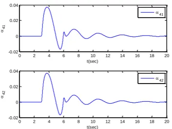
Figure 20. The slip angle of the fourth axle trailer in time in the single line switching maneuver

5. CONCLUSION

Regarding the fact that in recent years, less work has been done on modeling and controlling trailers themselves, especially trailers with multiple axles, in this research dynamic modeling and 5-axle trailer control were placed on the agenda. The first idea for increasing the trailer maneuver, improving its behavior, increasing the speed of the trailer in maneuvers, reducing the tire's tire speed and improving the system's control function to prevent the occurrence of Jack-Knifing phenomenon and other phenomena that cause trouble in controlling the trailer, driving ability axes are used. For this purpose, axle 1, 4 and 5 trailer are intended to be steering axles. In this paper, after introducing the 5 axis trailer system, a dynamic trailer modeling, which includes kinematics and trailer kinetics, was carried out and motor equations were extracted. Then, an optimal linear square control algorithm was introduced and based on this control algorithm, a controller for the trailer was designed. In order to ensure the operation of the control algorithm, several maneuvers were simulated. In the end, the simulation results were discussed on the results.

6. REFERENCES

1. Nuttall Jr, C., "Some notes on the steering of tracked vehicles by articulation", Journal of Terramechanics, Vol. 1, No. 1, (1964), 38-74.

3. Mashadi, B., Mahmoudi-Kaleybar, M., Ahmadizadeh, P. and Oveisi, A., "A path-following driver/vehicle model with optimized lateral dynamic controller", Latin American journal of Solids and Structures, Vol. 11, No. 4, (2014), 613-630.

4. Kar, M.K., "Prediction of track forces in skid-steering of military tracked vehicles", Journal of Terramechanics, Vol. 24, No. 1, (1987), 75-84.

5. Watanabe, K. and Kitano, M., "Study on steerability of articulated tracked vehicles—part 1. Theoretical and experimental analysis", Journal of Terramechanics, Vol. 23, No. 2, (1986), 69-83.

6. Montazeri-Gh, M. and Mahmoodi-K, M., "Optimized predictive energy management of plug-in hybrid electric vehicle based on traffic condition", Journal of Cleaner Production, Vol. 139, (2016), 935-948.

7. Alhimdani, F.F., "Steering analysis of articulated tracked vehicles", Journal of Terramechanics, Vol. 19, No. 3, (1982), 195-209.

8. Alhimdani, F. and Younis, B., "Effect of hydraulic piston on hinge force of wagon-type articulated tracked vehicle", in Proc. 10th Int. Conf. ISTVS. (1990), 843-855.

10. Luijten, M., "Lateral dynamic behaviour of articulated commercial vehicles", Eindhoven University of Technology, (2010).

11. Bouteldja, M. and Cerezo, V., "Jackknifing warning for articulated vehicles based on a detection and prediction system", in 3rd International Conference on Road Safety and Simulation, Indianapolis, USA, September. (2011).

12. Chen, C. and Tomizuka, M., "Modeling and control of articulated vehicles", UC Berkely, California, (1997).

13. Fancher, P. and Winkler, C., "Directional performance issues in evaluation and design of articulated heavy vehicles", Vehicle System Dynamics, Vol. 45, No. 7-8, (2007), 607-647.

14. Schmid, I., "Engineering approach to truck and tractor train stability", SAE Transactions, (1968), 1-26.

15. Fakoor, M., Kosari, A. and Jafarzadeh, M., "Revision on fuzzy artificial potential field for humanoid robot path planning in unknown environment", International Journal of Advanced Mechatronic Systems, Vol. 6, No. 4, (2015), 174-183. 16. Fakoor, M., Kosari, A. and Jafarzadeh, M., "Humanoid robot path

planning with fuzzy markov decision processes", Journal of Applied Research and Technology, Vol. 14, No. 5, (2016), 300-310.

0 2 4 6 8 10 12 14 16 18 20

-0.02 0 0.02 0.04

t(sec)

41

₄₁

0 2 4 6 8 10 12 14 16 18 20

-0.02 0 0.02 0.04

t(sec)

42

42

2. Nematollahisarvestani, A. and Shamloo, A., "Dynamics of a magnetically rotated micro swimmer inspired by paramecium metachronal wave", Progress in Biophysics and Molecular

Biology, (2018) in press,

https://doi.org/10.1016/j.pbiomolbio.2018.08.002.

Optimal Control of the Vehicle Path Following by Using Image Processing Approach

Y. Pourasad

Faculty of Electrical Engineering, Urmia university of Technology, Urmia, Iran

P A P E R I N F O

Paper history:

Received 11 November 2017

Received in revised form 13 December 2017 Accepted 17 Januray 2018

Keywords: Trailer Image Processing Path Following Steerability Optimal Control هدیکچ هزورما تیمها و وردوخ تاریثات ریگمشچ نآ رب متسیس لمح و لقن راکشآ تسا . هدافتسا زا اهرلیرت اب یارب ،روحم نیدنچ

لمح و لقن تازیهجت نیگنس تلوصحم و یرورض تسا . یرادیاپ و نامرف یریذپ رلیرت هروحم دنچ یکی زا لئاسم یلصا رد متسیس لمح و لقن تسا . ،نیاربانب رد نیا ،هلاقم یزاسلدم و لرتنک یکیمانید رلیرت 5 هروحم دروم یسررب رارق تفرگ . هب هولاع یریذپرونام دوبهب یارب تعرس و ،ندیشخب 3 روحم هب ناونع نامرف ریذپ رد رظن هتفرگ دندش . نینچمه اب هدافتسا زا شزادرپ یم یعس ،ریوصت ات دوش ریسم رلیرت رد ریسم هاوخلد اب نیرتلااب تقد ،روظنم نیدب .دریگرارق ادتبا لدم 14 هجرد یدازآ یارب رلیرت 5 یروحم اب 3 روحم نامرف ریذپ دروم یسررب رارق تفرگ و یکیمانید لدم نآ هئارا دش . ادتبا تلاداعم یکیمانید زا هلمج کیتامنیس و کیتنیس رلیرت تسدب هدمآ تسا . سپس اب یبایزرا خساپ ،رلیرت کی متیروگلا لرتنک هنیهب بولطم یطخ یحارط دش . هب روظنم یبایزرا درکلمع متیروگلا ،یلرتنک هیبش یزاس هلئسم لرتنک رونام یط رد و ریسم رییغت

ماجنا وردوخ نتفرگ تقبس دش

. جیاتن متیروگلا هک داد ناشن لرتنک و متسیس شزادرپ ارط ریوصت ح هدش ی ییاراک و تقد

.دراد ار درکلمع